Testing the Monte Carlo - Mean Field approximation in the one-band Hubbard model

Abstract

The canonical one-band Hubbard model is studied using a computational method that mixes the Monte Carlo procedure with the mean field approximation. This technique allows us to incorporate thermal fluctuations and the development of short-range magnetic order above ordering temperatures, contrary to the crude finite-temperature Hartree-Fock approximation, which incorrectly predicts a Néel temperature $T_{N}$ that grows linearly with the Hubbard $U/t$. The effective model studied here contains quantum and classical degrees of freedom. It thus belongs to the “spin fermion” model family widely employed in other contexts. Using exact diagonalization, supplemented by the traveling cluster approximation, for the fermionic sector, and classical Monte Carlo for the classical fields, the Hubbard $U/t$ vs. temperature $T/t$ phase diagram is studied employing large three and two dimensional clusters. We demonstrate that the method is capable of capturing the formation of local moments in the normal state without long-range order, the non-monotonicity of $T_{N}$ with increasing $U/t$, the development of gaps and pseudogaps in the density of states, and the two-peak structure in the specific heat. Extensive comparisons with determinant quantum Monte Carlo results suggest that the present approach is qualitatively, and often quantitatively, accurate, particularly at intermediate and high temperatures. Finally, we study the Hubbard model including plaquette diagonal hopping (i.e. the $t-t^{\prime}$ Hubbard model) in two dimensions and show that our approach allows us to study low temperature properties where determinant quantum Monte Carlo fails due to the fermion sign problem. Future applications of this method include multi-orbital Hubbard models such as those needed for iron-based superconductors.

I Introduction

The study of strongly correlated electrons continues attracting the interest of the condensed matter community.Tokura and Nagaosa (2000); Dagotto (2005) Theoretical studies in this area of research mainly use model Hamiltonians since there are no ab-initio techniques that can handle with sufficient accuracy the correlation effects caused by the Coulombic charge repulsion among the electrons. The case of the Hubbard model with only one active orbital ($d_{x^{2}-y^{2}}$) has been widely studied in the context of copper-based high temperature superconductors, and a variety of interesting results and predictions have been unveiled.Dagotto (1994); Scalapino (1995); Lee et al. (2006) A large fraction of those studies, however, arise from approximate analytic many-body techniques that are difficult to control since there is no obvious small parameter to guide expansions when one is dealing with correlated electrons. For this reason, considerable efforts have been devoted to the use of computational techniques to study Hubbard-like models.Dagotto (1994) Alas, these computational methods are not without severe limitations as well. For example, the Lanczos method is restricted to small clustersDagotto (1994) while the density matrix renormalization group (DMRG) is restricted to quasi one-dimensional systems.White (1992) An alternative is the determinant quantum Monte Carlo (DQMC) technique, Blankenbecler et al. (1981); White et al. (1989); Paiva et al. (2010) which can handle the one-orbital Hubbard model in dimensions larger than one and employing clusters of a reasonable size. This technique has been applied in numerous occasions, leading recently also to studies in the context of optical lattices.Bloch et al. (2008); Paiva et al. (2011); Kozik et al. (2013) DQMC presents the infamous “sign problem”, however, which severely restricts its range of applicability. For instance, deviations from the particle-hole symmetric model, such as when electronic hopping beyond nearest-neighbors are introduced, or when doping away from half-filling is attempted, severely restricts the temperature range where DQMC can be applied.Loh et al. (1990); White et al. (1989)

The limitations of our computational arsenal to deal with Hubbard-like models have been exposed even more dramatically by the recent discovery of the iron-based high temperature superconductors.Johnston (2010); Stewart (2011); Dai et al. (2012); Dagotto (2013) While considerable theoretical progress has been achieved in this context via the use of mean field approximations of several varieties,Johnston (2010); Stewart (2011); Dagotto (2013); Hirschfeld et al. (2011); Si and Abrahams (2008) computational work has been severely restricted. This is mainly because of the need to incorporate several $3d$ iron orbitals in the model Hamiltonian. It is well known that the Hubbard model for pnictides must have a minimum of two iron orbitals: $d_{xz}$ and $d_{yz}$, while most experts agree that at least a third orbital $d_{xy}$ should also be incorporated.Daghofer et al. (2010) Moreover, the crystal structure indicates that hopping amplitudes must involve both Fe-Fe nearest and next-nearest neighbors processes. All these factors are detrimental to the performance of Lanczos, DMRG, and DQMC techniques, and the applications of these methods have been limited in the context of the iron-based superconductors. In fact, in a recent review,Dai et al. (2012) a crude drawing of the phase diagram of a multi-orbital Hubbard model was sketched “by hand” based on physical expectations, but this prediction has yet to be confirmed due to the lack of reliable techniques for the calculations.

Motivated by the above mentioned difficulties in handling the full problem, simplified versions of multi-orbital Hubbard models have been recently used in a number of contexts. For instance, in the colossal magnetoresistive manganitesDagotto et al. (2001); Salamon and Jaime (2001) the Double Exchange (DE) model separates the five $3d$ orbitals of Mn into mobile and localized degrees of freedom.Dagotto et al. (2001) This is compatible with the splittings caused by the crystal field; thus the separation of mobile and localized carriers is natural. Moreover, it has been shown that the localized spins, related to the $t_{2g}$ orbitals, can be approximated accurately by a classical spin.Dagotto et al. (2001, 1998) Extensive studies employing computational Monte Carlo techniques have provided ample evidence that this type of models can properly capture the physics of manganites.Yunoki et al. (1998); Moreo et al. (1999); Kumar and Majumdar (2006a); Dong et al. (2008, 2009); Liang et al. (2011); Şen et al. (2012) In contrast, employing a full five-orbital Hubbard model would have been impractical for the manganese oxides.

The DE model is a well-known example of a more general family of models referred to as “spin fermion” models, where “spin” denotes the localized degree of freedom and “fermion” denotes the mobile one. As in the DE case, the localized spin is considered classically in practice to allow for reasonable computational studies. Historically, the success of the DE model treated computationally has inspired the use of spin-fermion models for the cuprates as well. Spin fermion models for Cu oxides are technically similar to DE models and they have been able to reproduce features of the one-orbital Hubbard model, such as the dominance of $d$-wave pairing tendencies away from half-filling.Buhler et al. (2000a, b); Moraghebi et al. (2001, 2002a, 2002b) A similar approach has been used in the context of the Bogoliubov de Gennes (BdG) equations, allowing for the study of regimes beyond weak coupling BCS.Mayr et al. (2005); Alvarez et al. (2005); Mayr et al. (2006); Alvarez and Dagotto (2008) It should be stressed that none of the spin-fermion models, either in the manganite or cuprate context, exhibit a sign problem. Thus, computational studies are possible at any electronic density, temperature, and range of electronic hopping. Moreover, in spin fermion models dynamical observables can be easily obtained, contrary to dynamical observables in full Hubbard models that require calculations in imaginary time and a subsequent transformation to real frequency.Jarrell and Gubernatis (1996)

Spin fermion models seem to capture the qualitative essence of Hubbard models. Typically, however, they are defined “by hand” in cases where the mobile-localized separation is intuitively expected but it is unclear how this separation truly occurs in practice. (This is contrary to the DE model, where $e_{g}$ and $t_{2g}$ orbitals clearly separate the mobile electrons from the localized electrons). Thus, a method for constructing spin-fermion models systematically from their parent Hubbard models is desirable. This also would reveal the relationship between the effective couplings in the spin-fermion models and those of the more fundamental Hubbard interactions such as the repulsion $U$.

In this publication we explore these issues in depth in the context of the repulsive one-orbital Hubbard model. The essence of the computational method described here is to setup the mean field equations for the problem at hand, and then raise the mean field parameters, such as the effective staggered magnetic field that appears for an antiferromagnetic (AFM) state, to the level of a classical variable, which is then treated via Monte Carlo simulations at finite temperatures. These classical variables play the role of the “spin” in the resulting spin-fermion-like model. For the “fermions” the resulting Hamiltonian is quadratic and can be solved numerically via library subroutines or other procedures. To our knowledge, the first time that this methodology was proposed was in a study of the competition between AFM and superconducting (SC) tendencies in the one-orbital Hubbard model.Mayr et al. (2006) In this earlier work, both the staggered AFM field and a complex field representing the SC order parameter deduced from the BdG equations were introduced and handled via Monte Carlo simulations. Similar studies involving competing AFM and SC states within the Heisenberg model were presented in Refs. Alvarez et al., 2005 and Alvarez and Dagotto, 2008. In more recent efforts, these main ideas were also independently derived in detailed studies of the Hubbard model on an anisotropic triangular latticeTiwari and Majumdar (2013a) and on a geometrically frustrated face centered cubic lattice.Tiwari and Majumdar (2013b) Applications of the same approach but for the case of an attractive Hubbard interaction (negative $U$) that leads to pairing and superconductivity have been reported in Refs. Mayr et al., 2005; Alvarez et al., 2005; Mayr et al., 2006; Alvarez and Dagotto, 2008; Tarat and Majumdar, 2014, 2014a, 2014b.

As we will show, an interesting result is that this computational procedure captures the highly non-trivial non-monotonic behavior of the Néel temperature $T_{N}$ with increasing Hubbard $U$ at half-filling, in excellent agreement with DQMC. This is a dramatic improvement over standard Hartree-Fock mean field techniques that incorrectly predict a smooth increase of $T_{N}$ with $U$. This “up and down” behavior of $T_{N}$ with $U$ was also observed recently in a similar study of the negative $U$ Hubbard model Tarat and Majumdar (2014a) (note that there is a mapping between positive and negative $U$), and in early studies of models for $d$-wave superconductivity with increasing pairing attraction.Mayr et al. (2005); Alvarez et al. (2005); Mayr et al. (2006) In addition, many other observables calculated within this approach, such as the specific heat, are in qualitative, and often quantitative, agreement with DQMC, as shown below. Moreover, the spin-fermion model also allows for the calculation of dynamical observables directly in real time and frequency. We demonstrate this here by calculating the single-particle density of states. Finally, we further examine the utility of this approach by examining the Hubbard model with longer range hopping. In this case, DQMC cannot be applied due to a severe fermion sign problem but the new method is successful.

In summary, the simple combination of Monte Carlo and mean field methods allows for a proper treatment of the temperature effects in Hubbard models, including the study of regimes where the relevant correlations, such as the spin correlations, are of short range in space. Although it will be computationally demanding, after the success of the test presented here and in the other publications cited above, the method will be ready to be implemented for multi-orbital Hubbard models of relevance in, e.g., iron superconductors, where virtually nothing is known about their thermodynamic behavior.

This paper is organized as follows. The Hubbard model and the technique are discussed in Sec. II. The technique is formally introduced by using the Hubbard-Stratonovich variables first employed in Ref. Tiwari and Majumdar, 2013a. The main results are presented in Sec. III, starting with the case of three dimensions and its comparison with DQMC. This is followed by a presentation of results for the two dimensional case, as well as results for a Hubbard model with hopping beyond nearest neighbors where DQMC suffers from a severe sign problem. We conclude in Sec. IV with a brief summary and outlook.

II Model $\&$ method

Let us start the specific application of the ideas outlined in the Introduction by considering the one-band Hubbard model defined below (in a standard notation):

$$H=H_{o}+H_{1}=-t\sum_{\langle i,j\rangle,\sigma}c^{\dagger}_{i,\sigma}c^{\phantom{\dagger}}_{j,\sigma}+U\sum_{i}n_{i,\uparrow}n_{i,\downarrow}$$ (1)

To setup the formalism, it is convenient to perform a rotationally invariant decoupling of the interaction term in the following manner:Schulz (1990)

$$n_{i,\uparrow}n_{i,\downarrow} = \frac{1}{4}(n_{i}^{2})-S_{iz}^{2}$$ (2)

$$= \frac{1}{4}(n_{i}^{2})-({\mathbb{S}}_{i}\cdot\hat{\Omega}_{i})^{2}.$$

Here, the spin operator is ${\mathbb{S}_{i}}=\frac{\hbar}{2}\sum_{\alpha,\beta}c^{\dagger}_{i,\alpha}{\mathbb{\sigma}}^{\phantom{\dagger}}_{\alpha,\beta}c^{\phantom{\dagger}}_{i,\beta}$, $\hbar=1$, $\{\sigma^{x},\sigma^{y},\sigma^{z}\}$ are the Pauli matrices, and $\hat{\Omega}$ is an arbitrary unit vector. In the previous identity, we have used the fact that $({\mathbb{S}}_{i}\cdot\hat{\Omega}_{i})^{2}=(S_{i,x})^{2}=(S_{i,y})^{2}=(S_{i,z})^{2}$. The expression in the last line of Eq. 2 is rotationally invariant since it is in terms of the scalars $n_{i}$ and the dot product between ${\mathbb{S}}_{i}$ and $\hat{\Omega}_{i}$. It should be noted that there are other possible decouplings, but the formula above is the only one whose saddle point leads to the correct Hartree-Fock equations after implementing a Hubbard-Stratonovich (HS) decomposition. Below we will use the notation followed in recent literature.Santos (2003). For the HS decomposition, let us start with the partition function $Z=Tre^{-\beta H}$. Here the trace is over all particle numbers and site occupations. $\beta=1/T$, with $k_{B}$ set to 1. We now divide the interval $[0,\beta]$ into $M$ equally spaced slices, defined by $\beta=M\Delta\tau$, separated by $\Delta\tau$ and labeled from 1 to $M$. For large M, $\Delta\tau$ is a small parameter and allows us to employ the Suzuki-Trotter decomposition, so that we can write $e^{-\beta(H_{o}+H_{1})}=(e^{-\Delta\tau H_{o}}e^{-\Delta\tau H_{1}})^{M}$ to first order in $\Delta\tau$. Then using Eq.(2) and the Hubbard-Stratonovich identity, $e^{-\Delta\tau U\sum_{i}[\frac{1}{4}(n_{i}^{2})-({\mathbb{S}}_{i}\cdot\hat{\Omega}_{i})^{2}]}$, for a generic time slice ${}^{\prime}l^{\prime}$, can be shown to be proportional to,

$$\int{d\phi_{i}(l)d\Delta_{i}(l)d^{2}\Omega_{i}(l)}\times\hskip 125.19194pt$$

$$e^{-\Delta\tau[\sum_{i}(\frac{\phi_{i}(l)^{2}}{U}+i\phi_{i}(l)n_{i}+\frac{{\Delta_{i}(l)}^{2}}{U}-2{\Delta_{i}(l)}\hat{\Omega}_{i}(l).{\mathbb{S}_{i}})]}$$

Here we have introduced two auxiliary fields, $\phi_{i}(l)$ which couples to the charge density, and $\Delta_{i}(l)$ that couples to the spin density. We note that the integration over unit vector, $\hat{\Omega}_{i}(l)$ at every site shows the SU(2) invariance explicitly. We further combine the product $\Delta_{i}(l)\hat{\Omega}_{i}(l)$ into a new vector auxiliary field, ${\mathbb{m}_{i}}(l)$ at every site. This nomenclature is used from now on. Using the above decoupling for the quartic term in the expression of the partition function, we can write:

$$Z=const.\times Tr\prod^{1}_{l=M}\int{d\phi_{i}(l)d^{3}m_{i}(l)}e^{-\Delta\tau[-t\sum_{\langle i,j\rangle,\sigma}c^{\dagger}_{i,\sigma}c^{\phantom{\dagger}}_{j,\sigma}+\sum_{i}(\frac{\phi_{i}(l)^{2}}{U}+i\phi_{i}(l)n_{i}+\frac{{\mathbb{m}_{i}(l)}^{2}}{U}-2{\mathbb{m}_{i}(l)}.{\mathbb{S}_{i}})]}$$ (3)

In the above, trace ‘Tr’ is over all particle numbers and site occupations as before . The continuous integrals are over the auxiliary fields, $\{\phi_{i}(l),{\mathbb{m}_{i}(l)}\}$ at every site and the argument $l$ denotes imaginary time slice label. The product over $l$ from M to 1 implies time ordered products over time slices, with the earlier times appearing to the right. Finally, the $d^{3}m_{i}(l)$ in the integral, implies integration over the amplitude and orientation of vector auxiliary fields, ${\mathbb{m}_{i}(l)}$.

This allows us to identify an effective Hamiltonian $H_{eff}$ in which fermions couple to auxialiary fields fluctuaing in both space and (imaginary) time. Typically this is the starting point of Quantum Monte Carlo (QMC) approaches. However for reasons discussed in the introduction, we take a different route by making the following approximations. (i) We drop the $\tau$ dependence of the HS auxiliary fields and (ii) we use the saddle point value $i\phi_{i}=\frac{U}{2}\langle n_{i}\rangle$. This allows us to extract the following effective Hamiltonian ($H_{eff}$) where the fermions couple to the “static” HS field ${\mathbb{m}_{i}}$ and to the average local charge density:

$$H_{eff} = H_{o}-\mu\sum_{i}n_{i}+\sum_{i}\frac{U}{2}\langle n_{i}\rangle n_{i}-\sum_{i}{\mathbb{m}_{i}}.{\mathbb{\sigma}_{i}}$$ (4)

$$+ \frac{1}{U}\sum_{i}{\mathbb{m}_{i}}^{2}-\frac{U}{4}\sum_{i}\langle n_{i}\rangle^{2}.$$

Here, $H_{o}$ contains the fermionic kinetic energy. The redefinition ${\mathbb{m}}_{i}\rightarrow\frac{U}{2}{\mathbb{m}}_{i}$ allows us to arrive to the final form of the effective Hamiltonian:

$$H_{eff} = H_{o}+\frac{U}{2}\sum_{i}(\langle n_{i}\rangle n_{i}-{\mathbb{m}_{i}}.{\mathbb{\sigma}_{i}})$$

$$+ \frac{U}{4}\sum_{i}({\mathbb{m}_{i}}^{2}-\langle n_{i}\rangle^{2})-\mu\sum_{i}n_{i},$$

which is our effective model belonging to the spin-fermion family.

It should be noted that $H_{eff}$ coincides with the mean-field Hamiltonian at $T=0$, where ${\mathbb{m}_{i}}$ has the interpretation of the local magnetization. As discussed in the Introduction, to study the model at finite temperature, we simulate $H_{eff}$ by sampling the ${\mathbb{m}_{i}}$ fields via a classical Monte Carlo (MC) procedure.Mayr et al. (2006); Tarat and Majumdar (2014); Tiwari and Majumdar (2013a) The main result of the present effort will arise when these MC results at finite temperature are compared against DQMC results. It will be demonstrated that retaining thermal fluctuations in the fields ${\mathbb{m}_{i}}$ leads to results well beyond simple Hartree-Fock mean field calculations at finite temperature $T$ and, more importantly, in good qualitative and sometimes quantitative agreement with DQMC.

While the HS fields are treated via MC methods, the quadratic fermionic sector still needs to be handled numerically. The simplest and most widely employed method, starting with efforts in the manganite community to study the double exchange model,Yunoki et al. (1998) is simply to carry out an exact diagonalization (ED) of the fermions in a fixed classical ${\mathbb{m}_{i}}$ background, employing library subroutines. The ${\mathbb{m}_{i}}$ variables are then updated with a standard classical MC procedure where updates are accepted/rejected using the Metropolis algorithm. At a fixed temperature, this process is repeated until a thermalized regime is reached where observables can be measured.

Similarly as with the majority of techniques dealing with strongly correlated electrons, here there is no small parameter controlling the approximation. In particular there is no rigorous proof of convergence or bounded errors. However, as long as the mean field approximation employed as the starting point of the approximation (in the present example the Hartree Fock method) captures the essence of the ground state, then it is reasonable to assume that the present method will treat correctly the thermal fluctuations and associated short-range order tendencies above the critical temperature.

In the present work, we consider the case of half filling, where the total density is fixed by adjusting the chemical potential $\mu$. The Hamiltonian is studied on cubic lattices with 4³ to 16³ sites and with periodic boundary conditions. The magnetic structure factors $S({\bf q})$ are used to perform finite lattice size scaling to extract thermodynamic Néel temperatures in 3D. Results obtained on two dimensional clusters will also be shown. All parameters are specified in units of the hopping $t$. In practice a total of 4000 MC system sweeps were performed: 2000 were used to thermalize the system, while the rest were used for calculating observables. A MC system sweep consists of sequentially visiting every lattice site and updating the local ${\mathbb{m}_{i}}$ vector followed by the fermionic ED, and then accepting/rejecting the proposed local field change following the Metropolis algorithm. The local density $\langle n_{i}\rangle$ is computed from the eigenvectors after each diagonalization. In our calculation, we start the simulation at high temperature with a random configuration of ${\mathbb{m}_{i}}$ variables and then cool down to lower temperatures. To study the formation of local moments, as explained below, we start the MC runs at $T/t=100$ and cool down in steps of $\Delta T/t=1$ up to $T/t=1$. From $T/t=1$ to 0.1, we use a step size of $0.1t$. Below this temperature, specifically from $0.1t$ to $0.005t$, we reduce further the interval and use $\Delta T/t=0.05$. This slow process allows us to avoid metastable states or obtaining results that depend substantially on the initial conditions of the calculation.

To characterize the Hubbard model, a number of observables are computed during the MC procedure. In particular, we calculate the density of states (DOS), $N(\omega)=\sum_{m}\delta(\omega-\omega_{m})$, where $\omega_{m}$ are the eigenvalues of the fermionic sector and the summation runs up to $2N^{3}$, i.e. the total number of eigenvalues of a $N^{3}$ system with spin. $N(\omega)$ is calculated by implementing the usual Lorentzian representation of the $\delta$ function. The broadening needed to obtain $N(\omega)$ from the Lorentzians is $\sim BW/2N^{2}$, where $BW$ is the fermionic bandwidth at $U=0$. Numerically for the 4³ system, the broadening is about $0.09t$. Two hundred $N(\omega)$ samples are obtained from the 2000 measurement system sweeps at every temperature. We discard 10 MC steps between measurements to reduce self-correlations in the data. The 200 $N(\omega)$ samples are used to obtain the thermally averaged $\langle N(\omega)\rangle_{T}$ at a fixed temperature. These are further averaged over data obtained from 10-20 independent runs with different random number seeds.

Information regarding the Néel AFM order expected at half-filling is obtained from the magnetic structure factor,

$$S({\mathbb{q}})=\frac{1}{N^{2}}\displaystyle\sum\limits_{i,j}e^{i{\mathbb{q}}\cdot({\mathbb{r}}_{i}-{\mathbb{r}}_{j})}\langle{{\mathbb{S}_{i}}\cdot{\mathbb{S}_{j}}}\rangle,$$ (6)

where ${\mathbb{q}}=\{\pi,\pi,\pi\}$ is the wavevector of interest. The spins ${\mathbb{S}_{i}}$ are constructed from the eigenvectors of the equilibrated configurations.

We also calculate the real space correlation function between the ${\mathbb{S}_{i}}$ vectors. This correlation function is defined as,

$$C(|{\mathbb{r}}|)=\frac{1}{P}\sum\limits_{|{\mathbb{r}}|=|{\mathbb{i}}-{\mathbb{j}}|,a}(-1)^{|{\mathbb{i}}-{\mathbb{j}}|}\langle S^{a}_{i}S^{a}_{j}\rangle.$$ (7)

In $C(|{\mathbb{r}}|)$ the summation runs over all P pairs of sites at a distance $|{\mathbb{r}}|$ and is normalized accordingly. The sum over $a$ runs over the three directions $x$, $y$, and $z$.

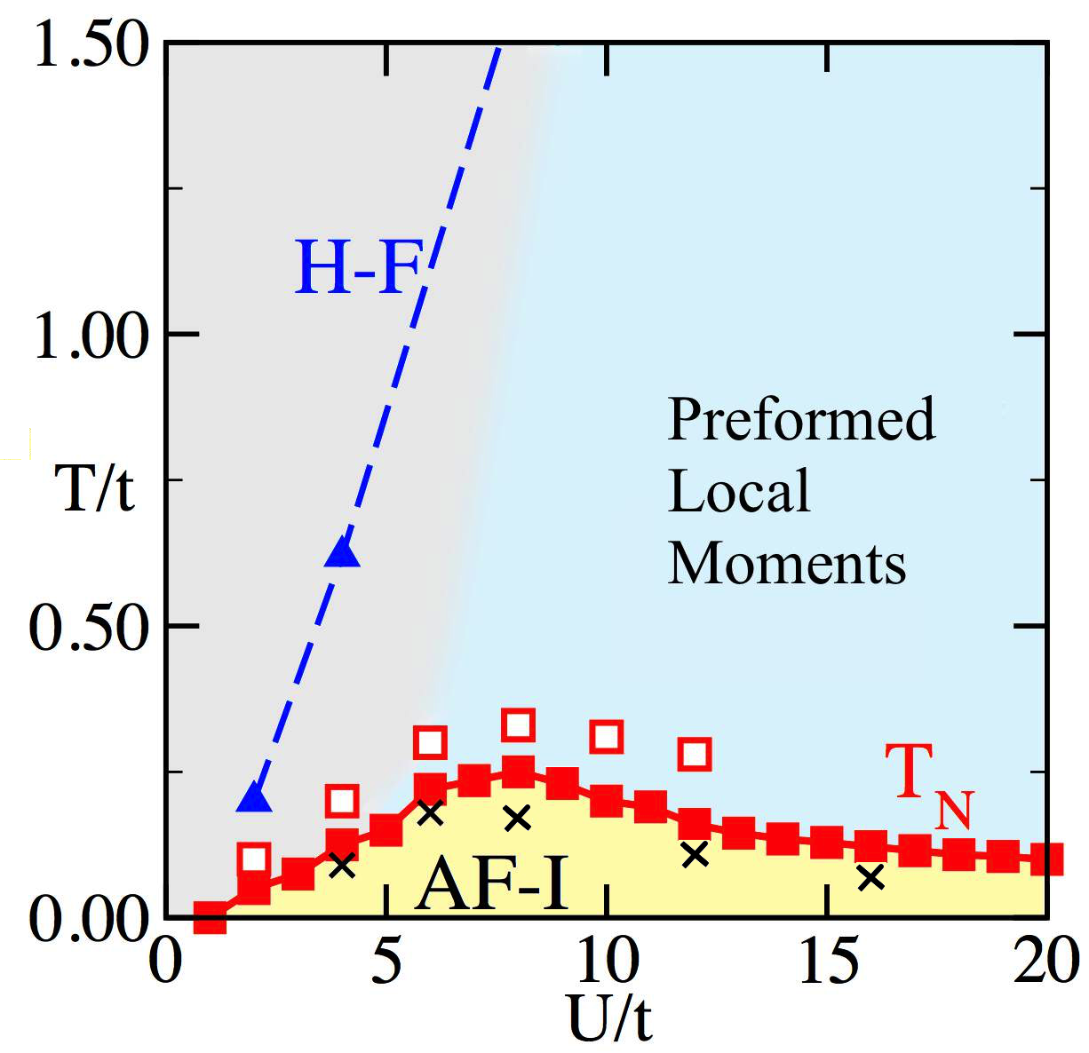
Figure 1: (color online) The $T/t-U/t$ phase diagram for the one-band Hubbard model. The solid red squares show the dependence of $T_{N}$ on $U/t$ obtained using the MCMF technique on $4^{3}$ clusters. The crosses are estimations of $T_{N}$ obtained from finite-size scaling. The AF-I region denotes the Néel type AFM phase with long-range order and insulating characteristics. The open squares are the $T_{N}$ obtained from the DQMC method, from Ref. Staudt et al., 2000. The light blue region depicts the regime of preformed local moments above the AF-I phase. The dashed line shows the $T_{N}$ obtained from the simplistic Hartree-Fock calculation at finite temperature where the critical temperature incorrectly grows linearly with $U/t$ at large $U/t$. The determination of the crossover between the gray and blue regions, and the fact that the MCMF local moment region coincides with HF $T_{N}$ at temperatures much larger than typical $T_{N}$ scales, are discussed in the text.

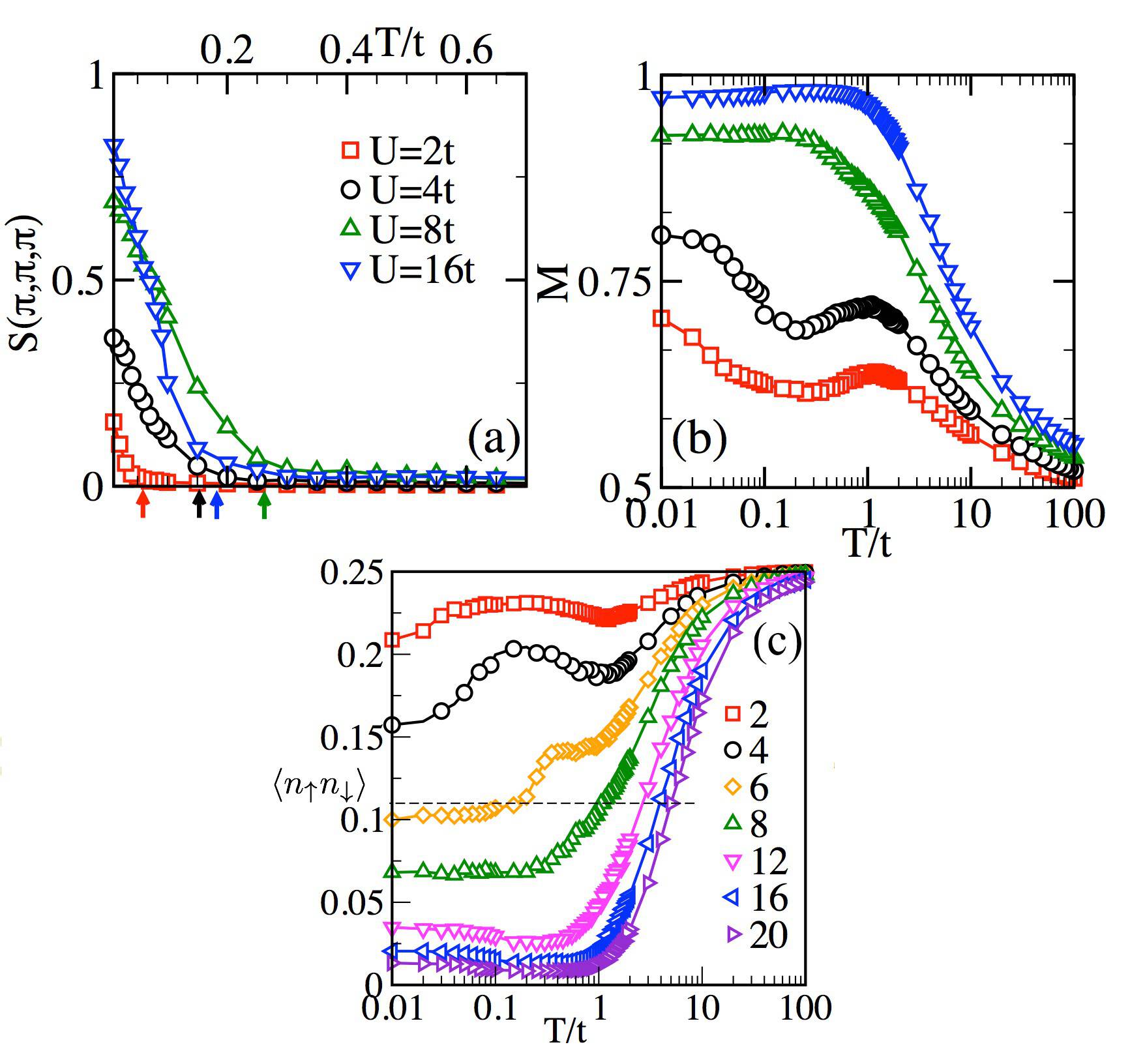
Figure 2: (color online) (a) The magnetic structure factor $S({\bf q})$ for ${\bf q}=(\pi,\pi,\pi)$, obtained at various $U/t$’s as indicated. The data is from 4³ clusters with 4000 MC sweeps at every temperature, while cooling the system down from high to low temperatures, as described in Sec. II. (b) The corresponding local moments, $M$, vs. temperature. We capture the feature that at large $U/t$ the peak in the moment size shifts to nonzero temperature. This effect, due to the setting of long range order, was reported before in the DQMC studies of Ref. Paiva et al., 2001. At small $U$ the overall shape is also in good agreement with the DQMC data, indicating that the MCMF method indeed captures the essence of the problem. (c) shows the expectation value of double occupation for the various $U/t$’s indicated. The thin dashed line indicates a cutoff discussed in the text.

The distribution of the magnitude of $|{\mathbb{m}_{i}}|$ on the lattice is measured by the distribution function $P_{q}(|{m}|)$. This is defined as $P_{q}(|{m}|)=\sum_{i}\delta(|m|-|{\mathbb{m}_{i}}|)$. For computational purposes, a Lorentzian representation with suitable broadening is used. $S({\mathbb{q}})$, $P_{q}(|{m}|)$, and $C(|{\mathbb{r}}|)$ are also averaged in the same manner as described for $N(\omega)$. We also compute the specific heat $C_{v}(U,T)=\frac{dE(U,T)}{dT}$ by numerically differentiating the average energy with respect to temperature. Other observables that we measured are presented below.

III Results

III.1 The Three Dimensional Lattice

Let us start the analysis of results with the $T/t-U/t$ phase diagram at half filling in 3D. In Fig. 1, we show the Néel temperature $T_{N}$ (solid squares; $4^{3}$ cluster) at different $U/t$’s obtained using the above described Monte Carlo - Mean Field (MCMF) method. The open squares are DQMC results, obtained from Ref. Staudt et al., 2000. The most important characteristic of the MCMF results is that they correctly capture the “up and down” non-monotonic behavior of $T_{N}$ with increasing $U$. In particular, comparing our results against the standard Hartree-Fock (HF) mean field theory predictions for $T_{N}$ (shown in dashed blue) highlights the crucial role of thermal fluctuations. These fluctuations break down the uniform mean-field order with varying degree of ease as $U/t$ is changed. The MCMF method includes thermal fluctuations and thus it correctly predicts the presence of a low energy scale (proportional to the Heisenberg superexchange $J$) that regulates the Néel temperature at large $U/t$, as opposed to the scale $U/t$ for $T_{N}$ favored by the “naive” HF method.

The comparison with DQMC also provides additional evidence that the new technique is not only qualitatively correct, but it provides reasonably quantitative values for $T_{N}$. The DQMC data shown are for up to 10³ clustersStaudt et al. (2000) while our MCMF data are shown for 4³ clusters via the red squares (results for larger lattices will be discussed below). Both capture the $t^{2}/U$ scaling of $T_{N}$ at large $U/t$. At small $U/t$, $T_{N}$ tends to zero with decreasing $U/t$ consistent with the $T_{N}\sim\exp[-2\pi t/U]$ scaling derived from the weak coupling random phase approximation.Tahvildar-Zadeh et al. (1997); Scalettar et al. (1989) The crosses are obtained from a finite-size scaling analysis of the results generated by the MCMF method, and represent $T_{N}$ in the thermodynamic limit. For numerical ease, we calculate the majority of the three dimensional data for 4³ systems, so to be consistent we show prominently the 4³ $T_{N}$ in Fig. 1. Finally, note that while the MCMF results are close to those of DQMC, the $T_{N}$ values are consistently underestimated in the present approach. Yet, qualitatively the MCMF results are correct. (Also note that Ref. Staudt et al., 2000 contains results of previous DQMC studies and the trend is that the predictions for $T_{N}$ are consistently decreasing with time as the results are more refined.) Nevertheless, for the purposes of testing the method (and in anticipation of the fact that the important application of MCMF will arise for multi-orbital systems where semiquantitative information will be sufficient due to the absence of DQMC), this degree of accuracy is quite acceptable.

Another important feature missing in the standard finite-temperature HF approach is the presence of local moments above $T_{N}$. The area shaded in blue in Fig. 1 shows the region with preformed local moments found with MCMF: the gray-blue boundary demarcates the crossover between regions with and without preformed local moments (it is just a crossover because the transition is smooth). The blue dashed line with triangles indicates the HF $T_{N}$, which also corresponds to the local moments formation in that crude mean-field approach. The crossover temperature increases monotonically with $U/t$ for $U\geq 6t$. At large $U$ it follows the HF $T_{N}$. Similar agreement has been reported in two dimensional DQMC results.Paiva et al. (2001) The determination of the crossover temperature and its systematics for $U<6t$ is discussed below.

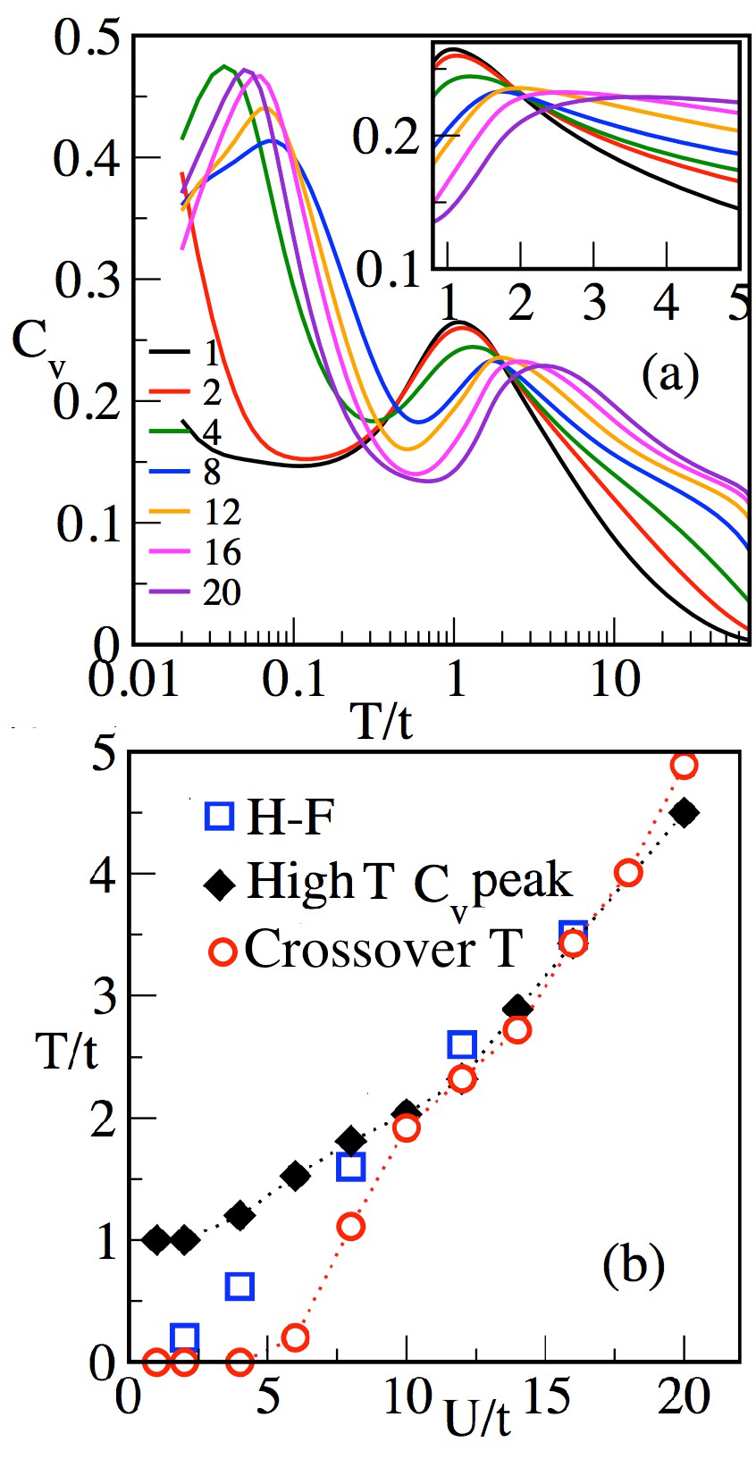
Figure 3: (color online) (a) Specific heat vs. temperatures for different $U$ values. Two peak structures are observed: at large $U/t$ the high-temperature peak corresponds to the moment formation while the lower one to moment ordering. The inset shows the universal crossing of the different $C_{v}$ curves at $T/t\sim 2.0$. (b) shows the position of the high-temperature peak varying $U$. The Hartree-Fock results are shown with open squares. At large $U$, beyond $6t$, these peak positions are close to the mean-field results. At low $U$, the high-temperature peak position saturates to $1t$, while the low-$T$ peak approaches zero. The non-merging of the two peaks in three dimensions is in agreement with DQMC data in 2D. The low-temperature peak correspond to $T_{N}$ in Fig. 1. The open circles in (b) show the crossover temperature from the no local moments regime to a region of preformed moments as obtained from the data on double occupation shown in Fig. 2 (c). In (a) the data shown is a smoothed version of the actual data to reduce statistical fluctuations.

(i) Local moments and magnetic order: Typical structure factors $S({\bf q})$ for ${\mathbb{q}}=(\pi,\pi,\pi)$ are shown in Fig. 2 (a). Here, we observe the non-monotonicity of $T_{N}$ with increasing $U$. This provide the finite size data for $T_{N}$ shown in Fig. 1. The moment formation vs. temperature is shown in panel (b). The system-averaged local moment is defined as $M=\langle(n_{\uparrow}-n_{\downarrow})^{2}\rangle=\langle n\rangle-2\langle n_{\uparrow}n_{\downarrow}\rangle$ with $\langle n\rangle=\langle n_{\uparrow}+n_{\downarrow}\rangle$. We note that for our rotation invariant case, $M=4\langle S_{z}^{2}\rangle=4\langle({\mathbb{S}}\cdot\hat{\Omega})^{2}\rangle$, where $\hat{\Omega}$ is an arbitrary unit vector.

For the half-filled $\langle n\rangle$=1 uncorrelated case $U=0$, $\langle n_{\uparrow}n_{\downarrow}\rangle=\langle n_{\uparrow}\rangle\langle n_{\downarrow}\rangle$=1/4. Thus for $U=0$, or alternatively $T/t\gg U/t$, $M=\frac{1}{2}$. This is seen in Fig. 2(b) at $T/t\sim 100$ for all values of $U/t$. From panel (c) we also observe that the average double occupation at high temperature for all $U/t$ values shown tends towards 0.25, the uncorrelated value of double occupancy. On the other hand, for large $U/t$ and very low $T/t$, the double occupation, $\langle n_{\uparrow}n_{\downarrow}\rangle$, is much suppressed and $M\sim 1$, i.e. the $U=\infty$ result. For any finite $U/t$ there is some finite double occupation and $M$ is always smaller that unity. Furthermore, since smaller $U/t$’s have larger double occupation, as shown in Fig. 2(c), $M(T\sim 0)$ monotonically decreases with reducing $U/t$, as shown in Fig. 2(b).

We also notice that $M(T)$ has some features at intermediate temperatures that evolve with $U/t$. In the intermediate temperature range, specifically between $T/t=1$ and $0.01$, we find two kinds of behavior. At small $U/t$, up to $U/t=4$, $M$ has a minima at $T/t\sim 0.2$ before reaching its absolute maximum at $T=0$. For larger $U$, the $M$ maxima lies at finite $T/t\sim 0.1$ and $\sim 0.5$, for $U/t=8$ and $16$, respectively. It is clear that for large $U/t$ the system can be approximated by a spin-1/2 Heisenberg antiferromagnet. Excitations at small but finite temperature that perturb the AFM order also suppress the virtual exchange due to the Pauli exclusion principle. This increases the degree of localization and promotes larger on-site moment size thereby pushing the maxima of $M$ to finite temperature. The features seen at low temperature for small $U$ are correlated to the thermal evolution of the fields updated with MC, as discussed later. Note that similar observations were reported before in two dimensional DQMC studies,Paiva et al. (2001) increasing the evidence that MCMF captures the essence of the problem.

(ii) Specific heat: The temperature evolution of the local moment in Fig. 2(b) shows a continuous increase with decreasing temperature up to $T/t=1$. But this does not provide clear information on the crossover location between regimes with and without local moments. To address this issue, and to further test the MCMF method, we calculated the specific heat $C_{v}$ vs. temperature for different values of $U$. Here, it is expected that $C_{v}$ vs. temperature should have a two peak structure, the peak at high temperature corresponding to moment formation and the peak at low temperature corresponds to moment ordering at large $U/t$.

In Fig. 3(a) the specific heat vs. temperature is shown for a 4³ system, where we find the expected two peak structure. The locus of the low-temperature peak corresponds well with the $T_{N}$ shown in Fig. 1. The high-temperature peak positions vs. $U/t$ are in Fig. 3(b). Here we also show the HF data with open squares. Clearly, beyond $U/t=10$ the MCMF result coincides with the HF result. At lower values of $U$ (below 4$t$), the high-temperature peak appears to saturate to $T/t=1$. On the other hand, the low-temperature peak is suppressed to zero with low $T$. We note that we were unable to reliably carry out the numerical derivative below $T/t=0.02$, but the trend of the low-temperature peak shifting towards zero is apparent here and is also in Fig. 1 (solid, red squares).

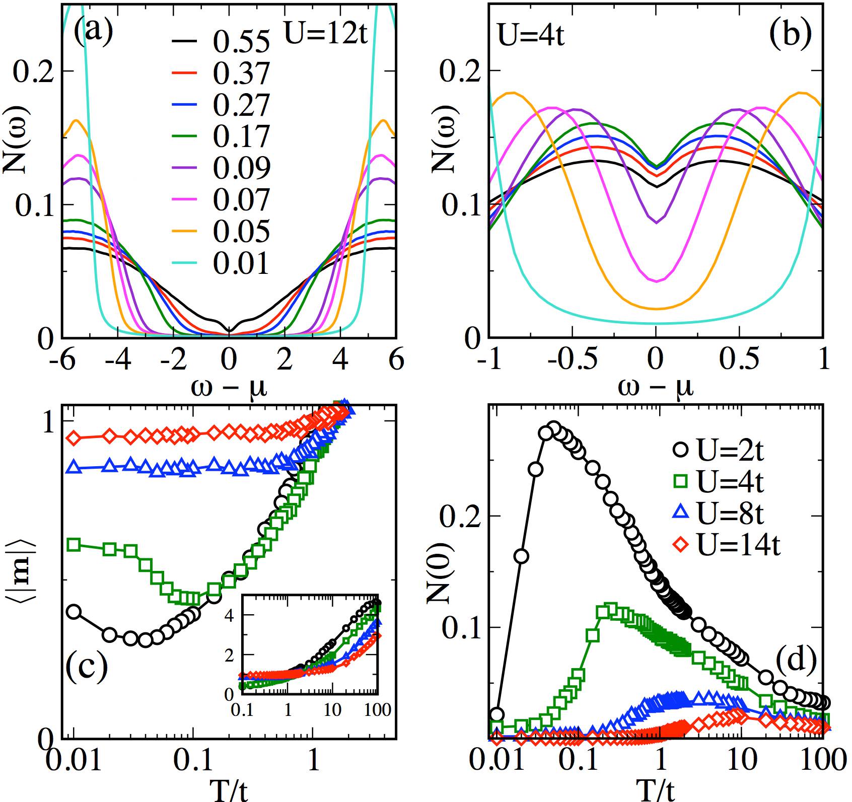
Figure 4: (color online) Density of states $N(\omega)$ for (a) $U/t=12$ and (b) $U/t=4$ at the temperatures indicated in panel (a). At large $U/t=12$, the Hubbard gap is gradually filled up due to thermal fluctuations. The weight at $\omega-\mu=0$ monotonically increases with increasing temperature. A DOS pseudogap is seen above $T_{N}\sim 0.2t$. At a smaller coupling $U/t(=4)$, while the gap is filled similarly to the large $U$ case with the increase of temperature, above $T_{N}$ we observe a non-monotonicity in the dependence of the zero-energy weight with temperature. (c) Magnitude of the auxiliary classical fields averaged over the lattice ($\langle|\textbf{m}|\rangle$) vs. temperature for the $U$ values in (d). At large temperature the thermal fluctuations cause ($\langle|\textbf{m}|\rangle$) to grow linearly with temperature for all the $U$’s shown (inset). The reason for this temperature dependence of $\langle|\textbf{m}|\rangle$ and its correlation with $N(\omega=0)$ is discussed in the text. (d) Shows the $N(\omega=0)$ feature remarked in panel (b) for different $U$ values. This non monotonicity was reported before in a DQMC study, see Ref. Paiva et al., 2001.

Thus, in the present study we report that the high- and low-temperature peaks do not merge with reducing temperature at small $U/t$ in three dimensions. (This is also the case in two dimensions, which is discussed later). Previous studies have not agreed on this issue: dynamical mean field theory (DMFT)Georges and Krauth (1993); Chandra et al. (1999); Vollhardt (1997) and Lanczos on one-dimensional chainsShiba and Pincus (1972) find the two peaks merging together with reducing $U$ while a DQMC study in two dimensionsPaiva et al. (2001), agrees with our conclusions. Here we have extended the results to three dimensions.

Another feature arising from the independence of the high-temperature entropyDuffy and Moreo (1997); Paiva et al. (2001) is a universal crossing in $C_{v}$. In two-dimensional DQMC, this occurs at $T/t\sim 1.6$, with a spread in temperature of $\sim 0.2t$. This has been observed in DMFTGeorges and Krauth (1993); Chandra et al. (1999); Vollhardt (1997) as well. We find a similar crossing both in three and two dimensions. In three dimensions the crossing is at approximately $T/t=2.0$ and has a small spread for low $U$ values, while at larger $U$ there seems to be a systematic increase to higher temperature with increasing $U$. This last conclusion was reported earlier as well.Duffy and Moreo (1997) For our main purpose of testing the MCMF method, in two dimensions once again our results agree well with DQMC data, as discussed later.

(iii) Crossover temperatures: At large $U$, the high-temperature peak of $C_{v}$ corresponds to the moment formation.Paiva et al. (2001) Thus, this peak is an indicator of the local moment formation temperature. Below $U/t=10$, however, this high-temperature peak deviates from the linear behavior seen in Fig. 3(b) and eventually saturates to $T/t=1$. The approach of the peak location to $T\sim t$ at small $U$ indicates that considerable contribution to this peak comes from electron delocalization. For this reason, for $U/t<10$, the high-temperature peak cannot be used as a reliable indicator of local moments. Thus, we use the double occupation, as plotted in Fig. 2(c), as an alternative indicator. To do so we need to choose a cutoff because the local moment formation is not abrupt but occurs with continuity. This cutoff is shown is Fig. 2(c) with the horizontal dashed line. For a given $U$, the temperature where double occupation goes below the cutoff is taken to be the crossover temperature to a region with preformed local moments. In principle the choice of such a cutoff is arbitrary, however, the $C_{v}$ calculation serves as a guide. To address this issue, we chose a cutoff value such that the location of the high-temperature peak in temperature and the crossover temperature from the cutoff coincide at large $U$ ($=18t$). The crossover temperature for all other $U$ values are obtained from this fixed cutoff. They are plotted in Fig. 3(b) with open circles. Clearly, there is a good agreement with the high-temperature $C_{v}$ peak locations for large $U$. For $U/t<10$, we find a sharp deviation from linearity in the crossover temperature. As seen from Fig. 2(c), the crossover temperature for $U/t=6$ is very close to the corresponding $T_{N}$ in Fig. 1. For lower $U$ values, for this choice of cutoff, large double occupation considerably suppresses the local moment formation.

(iv) Density of states: In the half-filled Hubbard model, the charge gap is directly related to the existence of the local moments regardless of magnetic order. This charge gap manifests as a gap (zero spectral weight in a finite energy range) in the DOS at $T=0$. With increasing temperature, this hard gap softens and is replaced by a pseudogap, with the spectral weight in the gap gradually increasing with increasing temperature. At large $U/t$ this monotonic behavior is seen in Fig. 4(a) from our MCMF results. The DOS is displayed up to $T=0.55t$, but the monotonicity persists to higher temperatures. In contrast, at $U/t=4$, shown in Fig. 4(b), the pseudogap spectral weight has a non-monotonic behavior: for $T>0.17t$ the spectral weight at $\omega-\mu=0$ decreases with increasing temperature, while for $T<0.17t$ the spectral weight decreases with decreasing temperature.

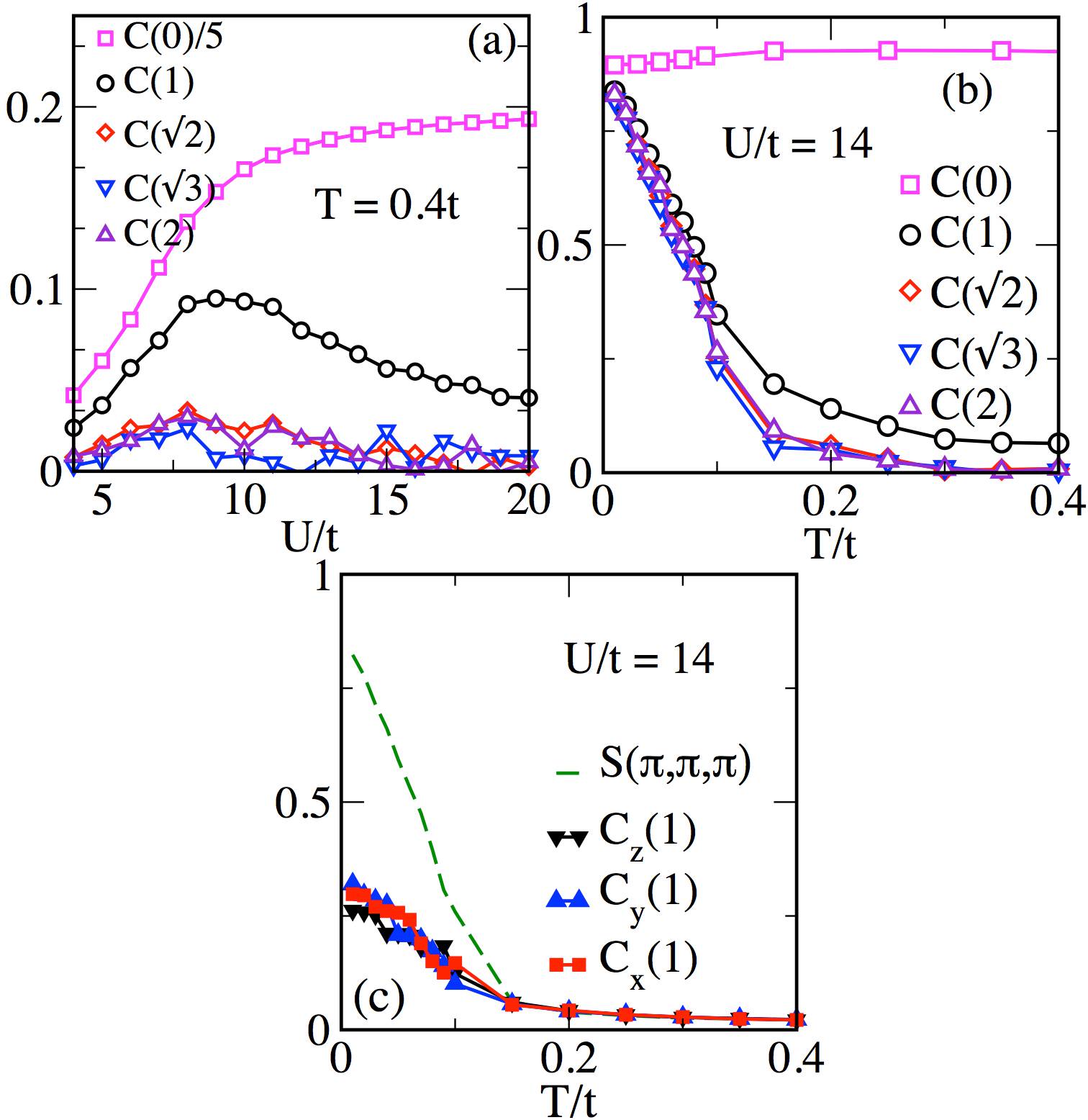
Figure 5: (color online) (a) Real space spin-spin correlations $C(|{\mathbb{r}}|)$, for $|{\mathbb{r}}|=0,1,\sqrt{2},\sqrt{3},2$, at $T/t=0.4$, i.e. a temperature above $T_{N}$. See the text for the definition of $C(|{\mathbb{r}}|)$. The $|{\mathbb{r}}|=0$ curve corresponds to the square of the local moment and shows that the size of the preformed magnetic moment increases with $U/t$ and saturates beyond $U/t\sim 8$, i.e. where $T_{N}$ is maximized. The rest of the curves show the real space AFM correlations, ${\mathbb{q}}=(\pi,\pi,\pi$), among the moments. Again the correlations are the largest for $U/t\sim 8$. On the large $U$ side the decrease in the correlation results from thermal fluctuations competing with the AFM spin order stiffness which scales as $t^{2}/U$. (b) Shows the dependence of $C(|{\mathbb{r}}|)$ on temperature for large $U/t(=14)$. The magnitude of the moment is almost independent of the temperature, while there is a clear short-range AFM correlation between the moments at all temperatures shown. Longer range correlations for $|{\mathbb{r}}|>1$ are suppressed rapidly above $T_{N}\sim 0.12t$. (c) The real-space correlations $C(|{\mathbb{r}}|=1)$ using only the $x$, $y$, or $z$ components of the spin. The data confirms explicitly the rotational invariance expected to exist in $H_{eff}$. The AFM structure factor is also displayed for comparison. Results are similar for $|{\mathbb{r}}|>1$ as well.

Since the spectral weight at $N(\omega=0)$ results from the scattering of the electrons from the classical fields, in Fig. 4(c) we show the evolution of the corresponding system-averaged auxiliary field values, $\langle|{\mathbb{m}}|\rangle$. For $U/t=2$ and 4, $\langle|\textbf{m}|\rangle$ has minima at $T/t=0.05$ and $0.1$, respectively. For $U/t=8$ and 14, $\langle|\textbf{m}|\rangle\sim 1$ for $T/t\lesssim$ 0.5.

The behavior shown in Fig. 4 can be explained as follows. At high enough temperatures with negligible local moments, the value of $\langle|\textbf{m}|\rangle$ is governed by thermal fluctuations. At these temperatures the auxiliary fields behave as harmonic oscillators with a mean amplitude proportional to $\sqrt{T/U}$. Thus, $\langle|\textbf{m}|\rangle$ grows with increasing temperature. On the other hand, the $T=0$ equilibrium value of $\langle|\textbf{m}|\rangle$ is directly proportional to $U$, as seen in Fig. 4(c). For smaller values of $U$, thermal fluctuations dominate to low enough temperatures, causing $\langle|\textbf{m}|\rangle$ to reduce to values smaller than their $T=0$ value. On further reduction in temperature, these thermal fluctuations are suppressed and $\langle|\textbf{m}|\rangle$ starts to increase towards its mean value at $T=0$. The minima in $\langle|\textbf{m}|\rangle$ vs. temperature corresponds to the location of the maxima in $N(0)$ in Fig. 4(d) for $U/t=2$ and 4. This indicates that the $N(0)$ suppression at high temperature results from the scattering of electrons from thermally fluctuating large $\{{\mathbb{m}_{i}}\}$ fields, while at small temperatures, the reduction in $N(0)$ results from the depletion of spectral weight due to the opening of the Mott gap. The peak in the $N(0)$ occurs between the two regimes.

With increasing $U$, the dominance of thermal fluctuations in governing $\langle|\textbf{m}|\rangle$ is pushed to progressively higher temperatures as is also seen from the peaks of $N(0)$ for $U/t=8$ and 16 in Fig. 4(d). At these temperatures $\langle|\textbf{m}|\rangle$ is higher than their $T=0$ values, thus no minima is found for these cases in Fig. 4(c).

We stress that the high temperature increase in the auxiliary field magnitude does not imply an increasing magnetic moment. As seen in Fig. 2(b) the magnetic moment $M$ saturates at its uncorrelated value of 1/2 at high temperature. The non-trivial effect of the fluctuations in the auxiliary fields is in the DOS, in the low-temperature feature in $M$ at small $U$, and possibly in the conductivity.

Another feature observed in the inset of Fig. 4(c) is that the magnitude of the auxiliary fields vs. temperature for different $U$’s cross between $T/t=1$ and $T/t=2$. Since at large $T$, $\langle|\textbf{m}|\rangle$ grows as $\sqrt{T/U}$, the auxiliary fields magnitude for smaller $U$ grows more rapidly than those for larger $U$. At small temperatures, however, the $\langle|\textbf{m}|\rangle$ values are directly proportional to $U$ as discussed before, naturally explaining the observed crossing. Note that this crossing coincides with the universal crossing of the specific heat in Fig. 3(a).

(v) Real space spin correlation: Figure 5(a) shows the spin-spin correlation $C(|{\mathbb{r}}|)$ at $T/t=0.4>T_{N}/t$ for different values of $|{\mathbb{r}}|$. The special case $|{\mathbb{r}}|=0$ corresponds to $M$ and with increasing $U/t$, $C(|{\mathbb{r}=0}|)$ saturates. The most prominent real space AFM correlation at this temperature is for $C(|{\mathbb{r}=1}|)$. While it is almost zero for $U/t\leq 4$, it increases as a function of $U/t$, reaches a maximum at $U\sim 8t$, and then reduces with further increases in $U/t$. The large $U/t$ suppression is due to the $t^{2}/U$ suppression of the spin ordering stiffness. While a similar trend is seen for larger $|{\mathbb{r}}|$, the magnitude of the correlation is greatly suppressed. In Fig. 5(b) we show the evolution of $C(|{\mathbb{r}}|)$ with temperature at a typical large value of $U/t$. While the magnitude of the moment, given by $C(|{\mathbb{r}=0}|)$, increases slightly with temperature, the short-range correlations are suppressed rapidly beyond $T_{N}$. The increase in $C(|{\mathbb{r}=0}|)$ or the size of the local moment were discussed earlier. Only $C(|{\mathbb{r}=1}|)$ is robust above $T_{N}$. Finally in Fig. 5(c) we also show individually the $x$, $y$, and $z$ components of $C(|{\mathbb{r}}|)$ for $|{\mathbb{r}}|=1$ for $U=14t$. This confirms explicitly the rotational invariance of the calculation.

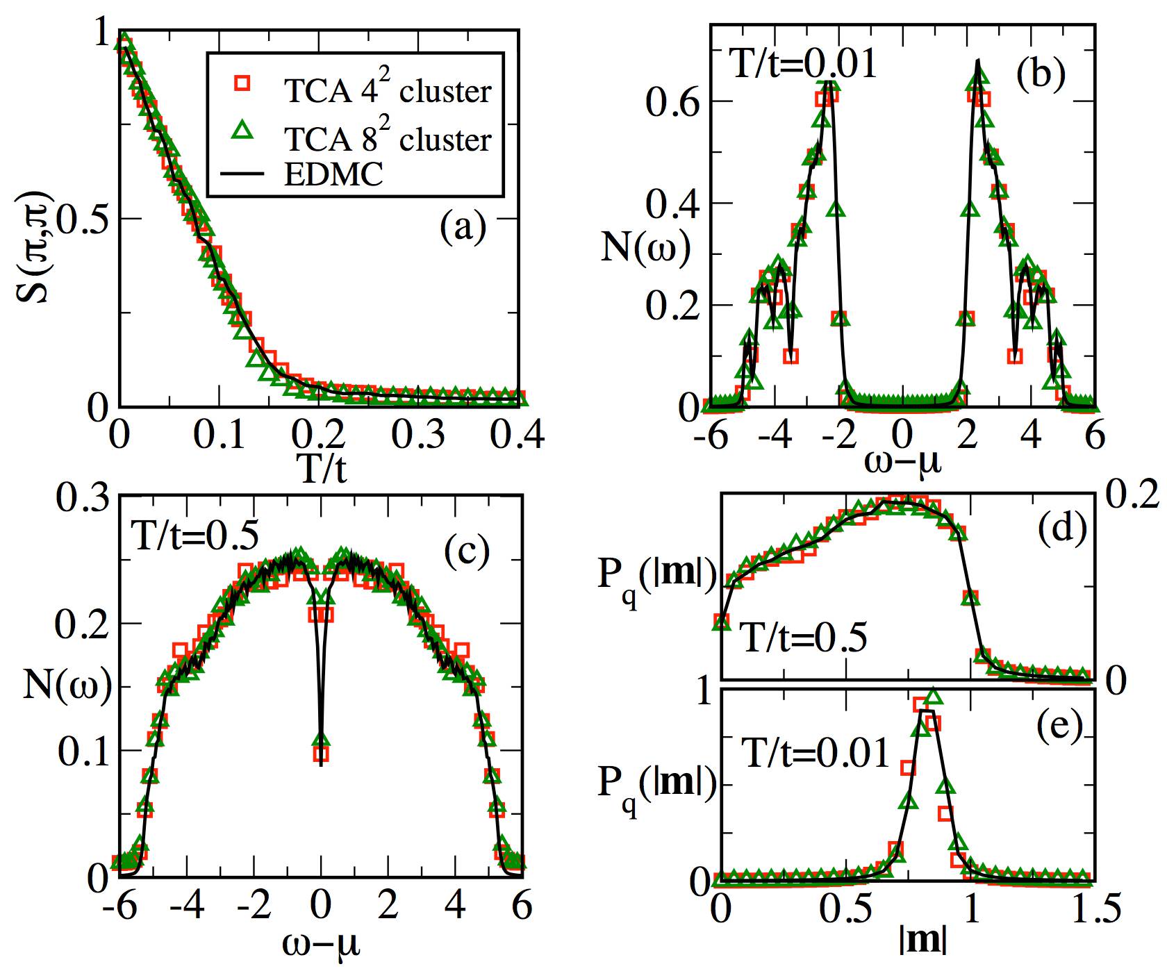
Figure 6: (color online) Comparison of results for an 8² system at $U/t=6$, obtained using ED+MC (solid line) and TCA with two different sizes of traveling cluster sizes, $4^{2}$ (squares) and $8^{2}$ (triangles). (a) shows $S(\pi,\pi)$, (b) and (c) show the DOS, while (d) and (e) display the $P_{q}(|{m}|)$, for the three cases. The DOS and $P_{q}(|{m}|)$ are shown at low $T(=0.01t)$ and high $T(=0.5t)$ temperatures, as indicated.

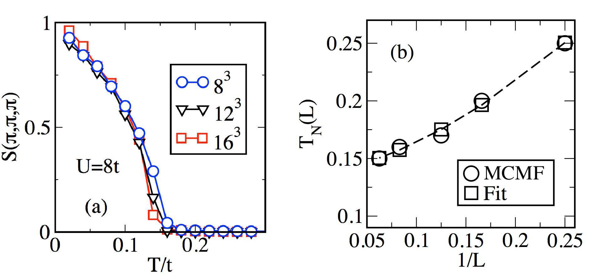
Figure 7: (color online) Finite size scaling analysis for the 3D case. (a) shows $S(\pi,\pi,\pi)$ for $U/t=8$ for three system sizes obtained using TCA. To find $T_{N}$ in the thermodynamic limit we fit $T_{N}(L)$, the Néel temperature for a cluster of size $L^{3}$, against 1/$L$. Fitting to a scaling form (see text) provides $T_{N}^{Thermo}$, the Néel temperature in the thermodynamic limit. As a typical example, in (b) we show the MCMF $T_{N}(L)$ data and the fit using the scaling form for $U=8t$ . The dashed line is a guide to the eye. See text for discussion.

Summarizing this subsection, we have established that the non-monotonic dependence of $T_{N}$ on $U$, the physics of preformed local moments, and the pseudogap features in the DOS can all be captured within the MCMF method.

III.2 Accessing larger system sizes

ED+MC is numerically expensive since an exact diagonalization must be performed at every step in the process. The numerical cost of a sequential sweep scales as $O(N^{3})\times N$, with $N$ the total number of lattice sites. To overcome this $O(N^{4})$ scaling we employ a recently developed variation of real space ED+MC that scales linearly with the system size.Kumar and Majumdar (2006b) This technique, called “Traveling Cluster Approximation” (TCA), defines a region (the traveling cluster) around the site where a MC update is attempted. A change is proposed and the update is accepted or rejected based on the energy change computed within the traveling cluster, thus bypassing the costly diagonalization of the full system. Only when observables are calculated, after equilibrium has been reached, is a full system diagonalization performed. This adds only a few hundred full system diagonalizations to the computational cost. For TCA, the computation cost of ED for a system with $N$ sites is $O(N_{c}^{3})$, where $N_{c}$ is the traveling cluster size. The cost of a full sweep of the lattice is $Nc^{3}\times N$ or linear in $N$ as opposed to $N^{4}$. This allows us to solve much larger systems. We now discuss our benchmarks for the TCA and the results on large two and three dimensional lattices.

1. Benchmarking: Let us begin by comparing the results from TCA with ED+MC. In Fig. 6 we compare various observables on two-dimensional 8² clusters with periodic boundary conditions. Results are shown for two different traveling cluster sizes, namely $N_{c}=4^{2}$ (squares) and $N_{c}=8^{2}$ (triangles), while results for the full ED + MC are given as the solid lines. Fig. 6(a) shows $S({\bf q})$ for ${\mathbb{q}}=(\pi,\pi)$, Figs. 6(b)-(c) show the DOS, and Figs. 6(d)-(e) show $P_{q}(|{\mathbb{m}}|)$ at low ($T=0.01t$) and high ($T=0.5t$) temperatures. All of the results are for $U=6t$. The $T_{N}$ obtained is about $0.15t$ from both methods. The Mott gap is found to be about $4t$ at low temperature [see 6(b)]. The pseudo gap feature at $T/t=0.5$ in Fig. 6(c) is also captured very accurately within TCA. Finally, all sites at low temperature show ${\mathbb{m}_{i}}\sim 1$ which evolves into a broad distribution at high temperatures. We find a satisfactory agreement between ED+MC and TCA data for all the observables and at all temperatures. Furthermore, these results show that employing a 4² traveling cluster is adequate as the results are virtually indistinguishable from those obtained using a 8² traveling cluster. In the following we will employ 4² and 4³ traveling clusters in two and three dimensions, respectively.

2. Finite size scaling: With TCA-based MCMF now we can study up to 16³ lattices. As a result the $S(\pi,\pi,\pi)$ data is available for $N=4^{3}$ to $16^{3}$ system sizes. Moreover, the magnetic structure factor obtained with the TCA agrees with the ED+MC data at all temperatures. This indicates that finite size effects associated with the TCA do not affect the finite temperature evolution of the magnetic state. Hence we can employ a finite size scaling analysis to the TCA data in order to obtain the Néel temperature in the thermodynamic limit.

On a finite system, estimates of T_N can be obtained either from an inspection of the $S(\pi,\pi,\pi)$ data or from the maxima of thermodynamic quantities such as the specific heat or the magnetic susceptibility. Then, assuming that the correlation length $\xi(T_{N}(L)-T_{N}^{Thermo})=aL$ on a $L^{3}$ system, and given that $\xi(x)\propto|x|^{-\nu}$, one arrives at the scaling form, $T_{N}(L)=T_{N}^{Thermo}+bL^{1/\nu}$. Here, $L$ denotes data from a $L^{3}$ cluster size. We plot the finite cluster Néel temperatures against $1/L$ and use $T_{N}^{Thermo}$, $b$, and $\nu$ as fit parameters. A typical data fit is presented in Fig. 7(b). For reference, we provide the $S(\pi,\pi,\pi)$ data for different system sizes in Fig. 7(a). The crosses in Fig. 1 are $T_{N}^{Thermo}$ obtained from this finite size scaling analysis.

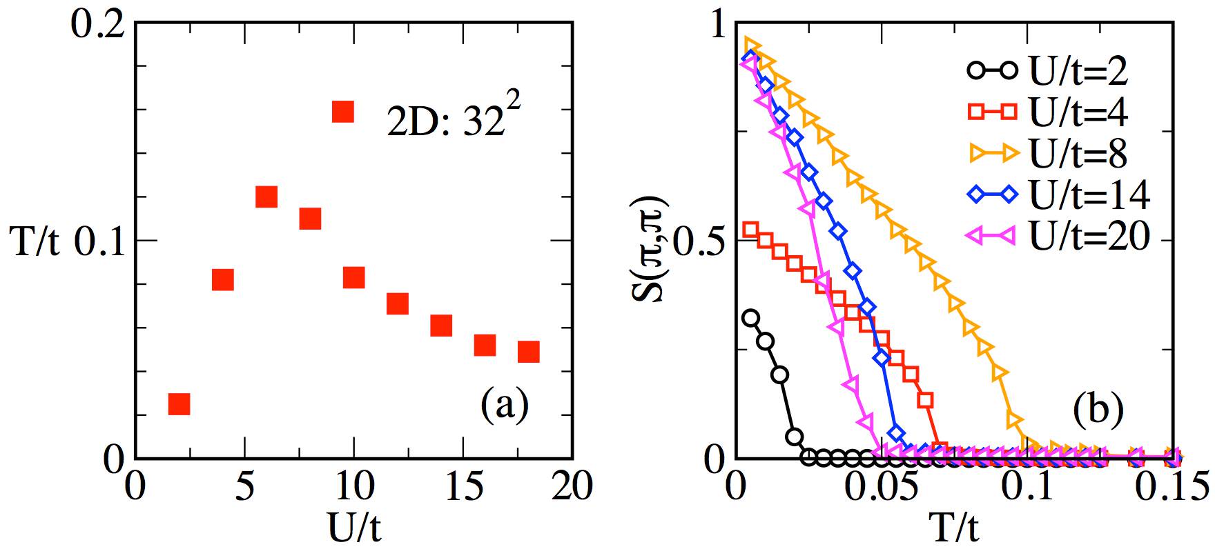
Figure 8: (color online) (a) $T_{N}$ vs $U/t$ and (b) representative $S(\pi,\pi)$’s, both for a 32² system. The results are obtained using a 4² traveling cluster.

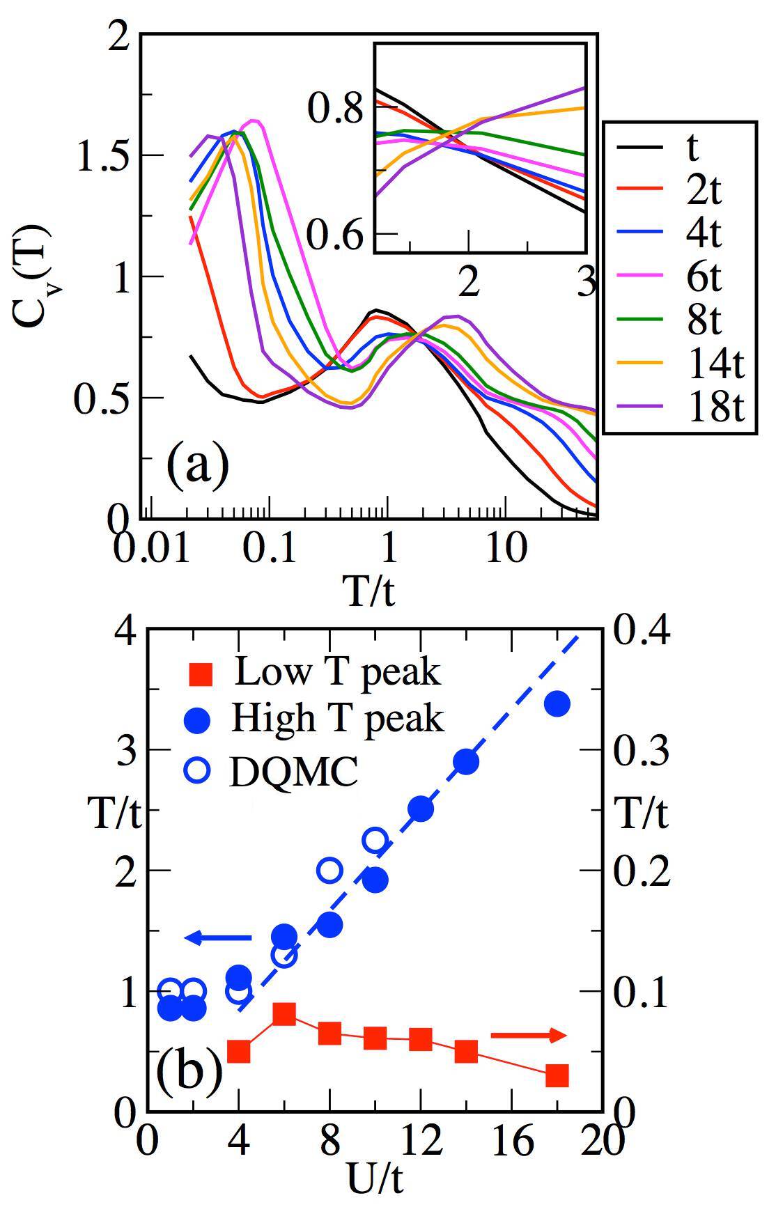
Figure 9: (color online) The specific heat vs temperature data in two dimensions for various $U$ values. The twin peak structure and universal crossing are clearly seen. The corresponding loci of the high- and low-temperature peaks are shown in (b). Here we also show DQMC data for the high-temperature peaks. For comparison with DQMC, we show this data for a 6² system size. The dashed line is a guide to the eye.

III.3 The two-dimensional lattice

We now turn to results for large two-dimensional system sizes using a 4² traveling cluster. The results shown in Fig. 8 are for a 32² system. The method can typically be pushed up to 40² sizes. Fig. 8(a) shows the AF Néel temperature. Note that in principle the Mermin-Wagner theorem establishes that there is no true $T_{N}$ in two dimensions for an $O(3)$ magnet. This theorem is valid only for short-range spin-spin interactions, however. In our case, the integration of the fermions leads to effective spin-spin interactions at all distances, although the rate of the decay of the couplings with distance is unknown. To be cautious we should refer to this scale as $T_{corr}$ instead of $T_{N}$, but below we will continue using the $T_{N}$ notation for this temperature scale since this is the convention widely used in the literature. Here, we observe that $T_{N}$ has the correct scaling of $t^{2}/U$ at large $U$. The corresponding spin structure factors are shown in Fig. 8(b).

To make a comparison with two dimensional DQMC data,Paiva et al. (2001) $C_{v}(T)$ as well as the locus of the high- and low-temperature peaks of the specific heat are shown in Fig. 9. As in the three dimensional case, we observe a two-peak structure in the specific heat and also capture the universal crossing of the $C_{v}(T)$ for different $U$ values in (a). The crossing occurs at $T/t=1.6$ and has a small spread in temperature values. These are in agreement with the DQMC data for the same system size. In 9(b) we show the comparison between our data and the peak locations in DQMC. We find that the saturation of the high-temperature peak ($T_{high}$) for $U/t<4$, persists in two dimensions. The small $U$ saturation of $T_{high}$ can be understood by studying the $U=0$ limit, where the specific heat peaks at $T\sim t(=1)$. For the behavior at large $U$ we can analyze the limiting case of $t=0$ (single site problem), where it is easy to see that $T_{high}$ grows linearly proportional to $U$. This linear growth of $T_{high}$ at large $U$ is seen in Fig. 9(b), and is in good agreement with DQMC results.Paiva et al. (2001)

The large system sizes accessible to MCMF allows a detailed analysis of the spatial evolution with temperature of the $\{{\mathbb{m}_{i}}\}$ field configurations, as shown in Fig. 10. Here, the top and bottom panels contain the spatial maps of $|{\mathbb{m}_{i}}|$ for $U/t=4$ and $14$, respectively. The maps are shown for four different temperatures, decreasing from left to right.

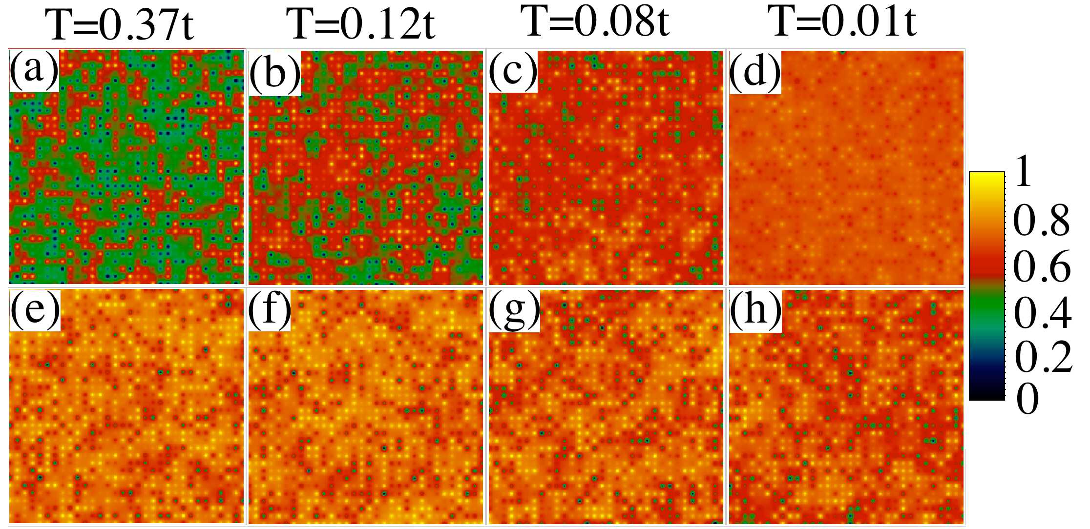
Figure 10: (color online) Spatial snapshots of $\{|{\mathbb{m}_{i}}|\}$ for $U/t=4$ (top) and $U/t=14$ (bottom). (a)-(d) and (e)-(h) show the snapshots for $T/t$=0.37, 0.12, 0.08, and 0.01 for the two cases, respectively. At $U/t=14$ (bottom), values as high as $|{\mathbb{m}}|\sim 1.0$ exist at all temperatures shown, much above $T_{N}(\sim 0.06t)$. $|{\mathbb{m}}|$, however, grows with reducing temperature and shows thermal fluctuations at the higher temperatures for $U/t=4$ (top). In the figure, yellow implies $|{\mathbb{m}}|=1$ and black $|{\mathbb{m}}|=0$. The snapshots are for a $32^{2}$ system size.

The temperature range here was chosen to show that in the small $U$ case the $\{{\mathbb{m}_{i}}\}$ grows with decreasing temperature, similar to the case in three dimensions. The strong thermal fluctuations that make the MCMF approach accurate at high temperatures are clearly visible. At $U/t=4$, the magnitude of $|{\mathbb{m}}|$ has a broad distribution, with regions of small and large values [see Fig. 10(a)]. At temperatures above but close to $T_{N}\sim 0.08t$, regions with $|{\mathbb{m}}|\sim 0.7$ start spanning the entire system, as exemplified in Figs. 10(b) and 10(c). Fig. 10(d) shows the system below $T_{N}$. These thermal fluctuations imply fluctuating spin moments in a MC snapshot, however, averaging over spin moments from many such MCMF configurations, at a fixed temperature, results in moments that are uniform in space. We stress that there is no spatial phase separation implied in these snapshots.

The corresponding distribution of the $\{{\mathbb{m}_{i}}\}$ configurations for Fig. 10 is shown in Fig. 11. In Fig. 11(a), we observe a gradual increase in the sharpness and peak height of $P_{q}(|{m}|)$ with reducing temperature. At large $U$, $P_{q}(|{m}|)$ shows little thermal fluctuations in the temperature range shown. This corresponds to almost saturated $\langle{\mathbb{|}m|}\rangle$ as in three dimensions at temperatures below $T/t\sim 1$. The uniformity in the bottom panel of Fig. 10 translates into a sharp $P_{q}(|{m}|)$ in Fig. 11 for a typical large values of $U/t$, as shown in Fig. 11(b) for $U/t=14$.

III.4 The half-filled Hubbard model with longer-range hopping

In this section we extend our analysis and apply the MCMF method to study the Hubbard model on a two-dimensional square lattice with nearest neighbor and next-nearest-neighbor hopping $t$ and $t^{\prime}$, respectively. The $t^{\prime}$ hopping processes have been widely considered important in the context of the cuprate superconductors, both directly in the Hubbard model,Duffy et al. (1997) as well as in the $t-t^{\prime}-J$ model.Nazarenko et al. (1995) In addition, understanding the role of $t^{\prime}$ is in general relevant to the study of frustrated systems. For this model DQMC studies, suffer a severe fermion sign problem due to the broken particle-hole symmetry introduced by $t^{\prime}$. Thus, the ground state properties remain inaccessible. DMFT studies have had more success but with limited or no spatial correlations.Sentef et al. (2011) There are other approaches to access the ground state properties,Tocchio et al. (2008); Becca et al. (2009); Markiewicz et al. (2010) but they are difficult to generalize to finite temperature. MCMF can fill this void.

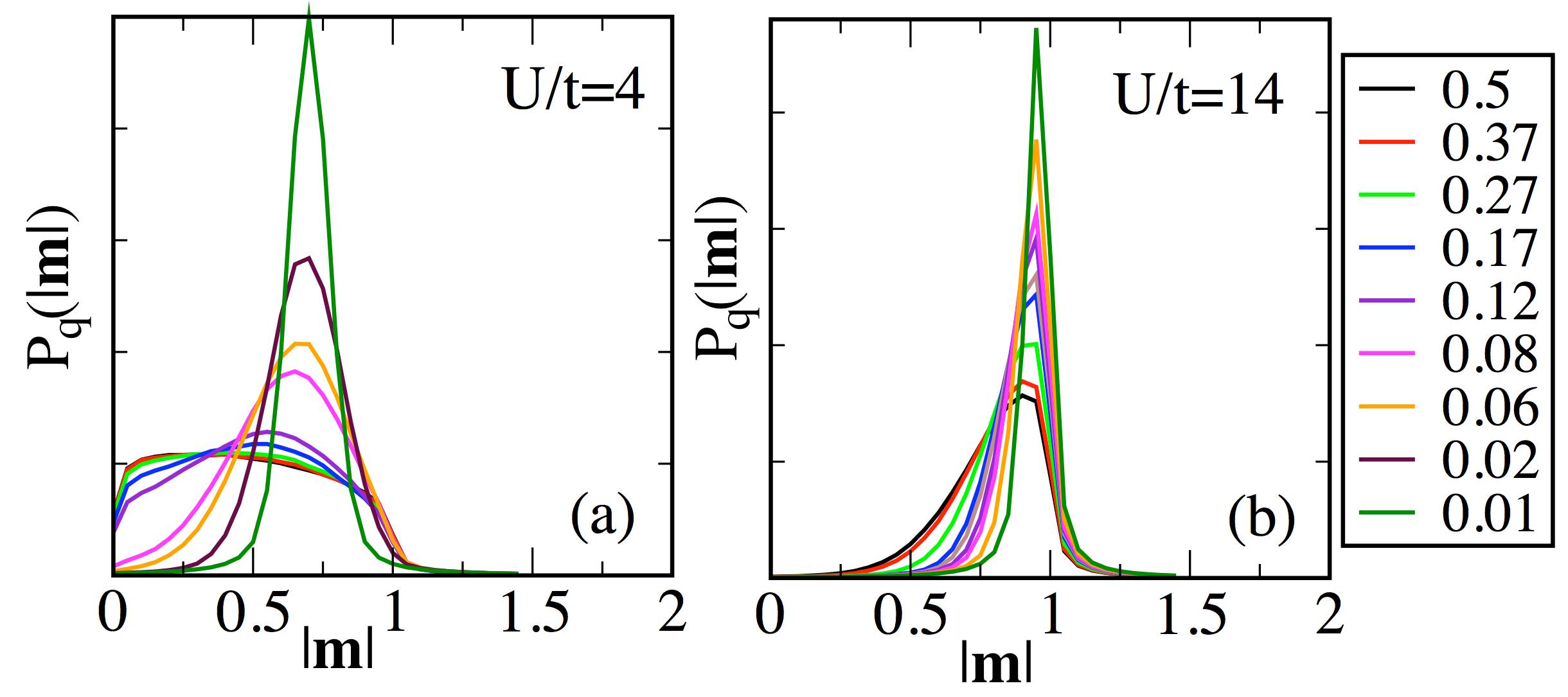
Figure 11: (color online) $P_{q}(|{m}|)$ for $U/t=4$ and 14 at various temperatures indicated on the right. (a) At $U/t=4$ and high temperature, lattice sites acquire values of $|{\mathbb{m}}|$ between 0 and 1 in a uniform manner. This distribution starts peaking at $T/t\sim 0.08$ which is close to $T_{N}$. At lower $T$, the auxiliary field distribution peaks at about $|{\mathbb{m}}|=$0.7. (b) At large $U/t$, the $|{\mathbb{m}}|$ values are well defined moments (about 1) at all sites at the temperatures shown, much above $T_{N}$. There is only a small thermal broadening even at $T\sim 10T_{N}$.

The MCMF approach used here reduces to unrestricted Hartree-Fock at $T=0$, but, as shown by comparison with DQMC results earlier, it rapidly improves its accuracy with increasing temperature. Moreover, MCMF does not have a sign problem. Thus, it allows controlled calculations of both finite temperature and ground state properties on very large two and three dimensional clusters, under a broad variety of circumstances. With this in mind, here we address the $U-t-t^{\prime}$ model using MCMF. We also use DQMC to solve the same problem for the lowest temperature allowed by the sign problem.

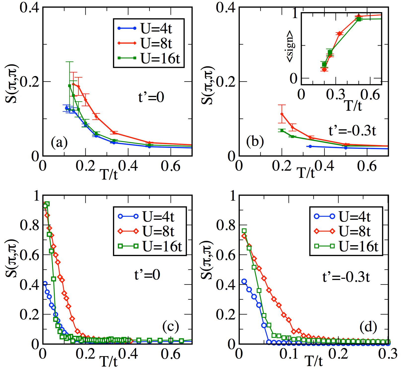
Figure 12: (color online) DQMC results showing $S(\pi,\pi)$ for several $U$’s at (a) $t^{\prime}=0$ and (b) $t^{\prime}=-0.3t$. The inset in (b) contains the average sign vs. temperature. For $t^{\prime}=-0.3t$, sign error increases rapidly preventing the access to low temperatures. (c) and (d) show the $S(\pi,\pi)$ obtained from MCMF. The data shown here is for a 6² system.

1. Comparison with DQMC : In Figs. 12(a) and 12(c), we show $S(\pi,\pi)$ calculated using DQMC and MCMF, respectively, for $t^{\prime}=0$. For this case, DQMC does not have sign problems and in principle we could obtain results for lower temperatures. However, given the $(O(L)^{2})$ scaling in CPU time (where $L$ is the number of imaginary time slicesWhite et al. (1989)) and the existence of results in the literature, we stopped the DQMC calculation at $T/t\sim 0.1$. It is clear that even at these temperatures we do observe AFM correlations beginning to grow with reducing $T$. We also observe that magnetic correlations begin to grow at a higher temperature for $U/t=8$ compared to $U/t=$ 4 and 16. This is indicative of the non-monotonicity of $T_{N}$ with $U$, as extensively discussed earlier. By comparison, MCMF ordering happens at a lower temperature. An additional difference with DQMC is the high temperature tail seen in 12(a), which is absent in 12(c). As shown for three dimensions in Fig 5(b), however, short range spatial correlation, in particular C($|{\mathbb{r}}=1|$), survives up to high temperatures. Similar correlations survive in two dimensions as well, but the presence of quantum effects makes the AFM correlations survive to longer length scales in DQMC contributing to the high temperature tail. In contrast, since only C($|{\mathbb{r}}=1|$) is significant in MCMF, the magnetic structure factor in 12(c) has a suppressed tail. This comparison highlights the effect of the mean field approximation in MCMF at low $T$ on long-range correlations and may explain the reduced values of $T_{N}$ as compared with DQMC.

In Fig. 12(b) we present $S(\pi,\pi)$ for the physically relevant case $t^{\prime}/t=-0.3$.Dagotto (1994) In the inset, we show the average value of the fermion sign as a function of temperature. The loss of particle-hole symmetry causes the average sign to rapidly fall to zero. As a result it becomes impossible to obtain reliable results below $T/t=0.2$ using DQMC. In contrast, the MCMF approach easily captures the long-range AFM order as shown in 12(d).

2. Ground state properties:

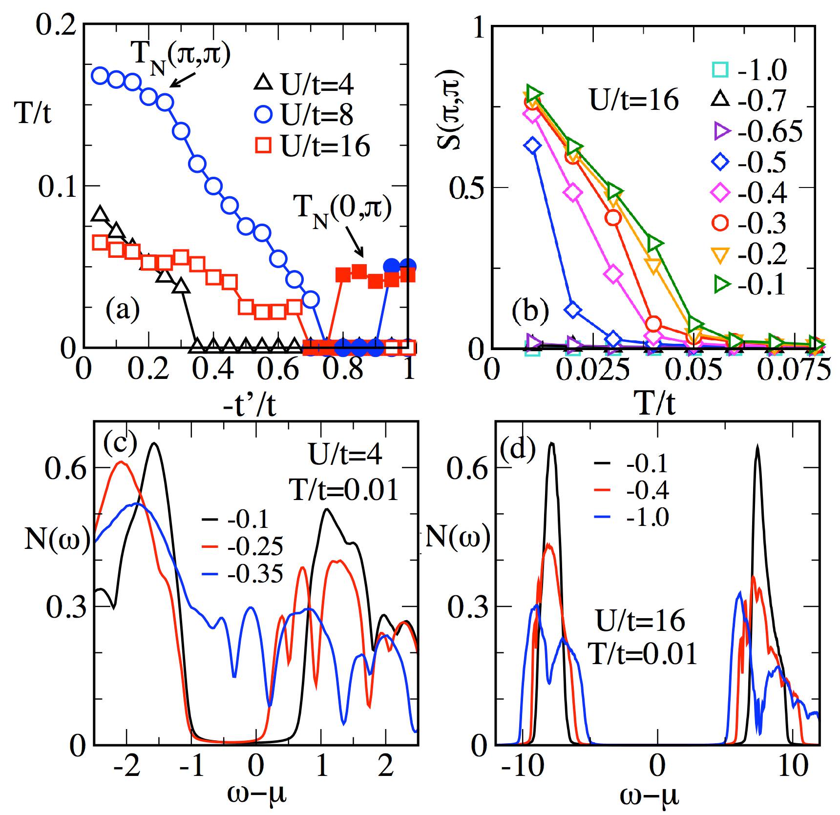
Figure 13: (color online) MCMF results for $t^{\prime}\neq 0$. Panel (a) contains the evolution of $T_{N}$ with increasing $t^{\prime}/t$ for different values of $U/t$ and for $\textbf{q}=(\pi,\pi)$ and $\textbf{q}=(0,\pi)$. The case $\textbf{q}=(\pi,0)$ is identical to $\textbf{q}=(0,\pi)$ and it is not shown. Panel (b) displays the typical $S(\pi,\pi)$ for $U/t=16$ at various $t^{\prime}/t$, as indicated. (c) and (d) show $N(\omega)$ for $U/t=4$ and $U/t=16$ respectively, at different values of $t^{\prime}/t$.

Earlier $T=0$ studiesTocchio et al. (2008); Becca et al. (2009); Markiewicz et al. (2010) have established that at small $U$, a small finite $t^{\prime}$ destroys magnetic order in favor of paramagnetism (PM). For $t^{\prime}/t$ below 0.7, the paramagnetic phase evolves into a $\textbf{q}=(\pi,\pi)$ antiferromagnet with increasing $U$. At larger $t^{\prime}$ and larger $U$, there is a transition to a state that is a linear superposition of $\textbf{q}=(0,\pi)$ and $\textbf{q}=(\pi,0)$ states from the PM state. Finally for $U$ greater than $10t$, there is a possible spin liquid phase in between the $\textbf{q}=(\pi,\pi)$ and $\textbf{q}=(0,\pi)$/$\textbf{q}=(\pi,0)$ phases. The Gutzwiller approximation combined with the random phase approximation (GA+RPA) also find a number of incommensurate magnetic phases sandwiched between the low $U$ (PM) and large $U$ ($\textbf{q}=(\pi,\pi)$ or $\textbf{q}=(0,\pi)$/$\textbf{q}=(\pi,0)$) orders.Markiewicz et al. (2010)

Here, we present some of the ground state and finite temperature properties with the goal to show the ability of MCMF to capture essential physics both at low and high temperatures. Detailed quantitative comparison with existing literature will be presented elsewhere. Figure 13 shows our results. In 13(a), the locus of the $\textbf{q}=(\pi,\pi)$ and $\textbf{q}=(0,\pi)$ Néel temperatures is shown as a function of $t^{\prime}/t$. The $U/t$ values used represent small, intermediate, and large $U/t$ regimes. At $U/t=4$, the $\textbf{q}=(\pi,\pi)$ phase is progressively weakened and ultimately destroyed in favor of a paramagnetic state. In 13(c) we show the DOS for $U/t=4$. At $t^{\prime}/t\sim-0.35$, there is an insulator to metal transition accompanying the magnetic to PM transition. For $U/t=8$ and 16, there is a similar loss of the $\textbf{q}=(\pi,\pi)$ magnetic order with increasing $t^{\prime}/t$. The critical $t^{\prime}/t$ needed shows non-monotonic dependence on $U/t$ similar to that of $T_{N}$ with varying $U/t$. The collapse of the $\textbf{q}=(\pi,\pi)$ order with increasing $t^{\prime}/t$ is shown in Fig. 13(b) for $U/t=16$.

In Fig. 13(d), the DOS for $U/t=16$ is presented. Clearly, the gap in N($\omega$) changes only slightly with $t^{\prime}/t$ varying from 0 to -1. A similar evolution occurs for $U/t=8$ as well. The gap survives because there is a transition from $\textbf{q}=(\pi,\pi)$ to a linear combination of the $\textbf{q}=(0,\pi)$/$\textbf{q}=(\pi,0)$. The locus of the peak of $\textbf{q}=(0,\pi)$ is shown in 13(a). In the region in between the two phases we only find a weak order difficult to distinguish from a PM state. Note that since this method reduces to the HF theory at $T=0$, a spin liquid phase cannot be captured within this approach due to the lack of quantum fluctuations; however, the MCMF method is able to suggest regions in parameter space where spin liquid phases are possible.

IV Conclusions

In this publication, a many-body technique which is “intermediate” between the canonical mean field Hartree-Fock approximation and the numerically exact determinant quantum Monte Carlo method has been discussed and tested for the case of the one-band Hubbard model. The thermal fluctuations that are properly considered in this method were shown to be sufficient to reproduce the expected “up and down” non-monotonic behavior of the Néel temperature with increasing $U/t$ at half-filling, unveiling a normal state regime where there are preformed local moments but no magnetic long-range order.

A necessary condition for the new method to work properly is that the mean field approximation used (either the HF method employed here or some other mean field method) captures the essence of the ground state magnetic, orbital, or even superconducting properties. After that step, the MC-MF technique is expected to address reasonably well the temperature fluctuations and generation of short-range order near the critical temperature. There are no obvious restrictions in parameters such as couplings: if the mean field method works at a particular coupling, the MC-MF will work as well varying the temperature. The coupling range where the method works best, in the sense of improving substantially over naive mean-field finite-T approximations, is strong coupling where fluctuations start developing when cooling down at temperatures much higher than the true long-range order critical temperature. Our technique captures the regime where local moments are formed but they are coupled effectively only at short distances. In superconducting systems with strong attraction, the method would capture the formation of individual Cooper pairs upon cooling, followed at lower temperatures by the true superconducting state.

Another advantage of the MCMF method is that it can be applied to other Hubbard models that cannot be treated by DQMC due to the fermion sign problem. As in the case of the addition of realistic $t’<0$ next nearest neighbor hopping amplitudes where DQMC can not reach the ordering temperature upon cooling because of the sign problem, the good performance of the MC-MF remains unchanged with regards to the case t’=0. Thus, examples where the MC-MF approach can be applied include the one-orbital Hubbard model with hopping beyond nearest neighbors, as demonstrated here, or the multi-orbital Hubbard models that are widely discussed for iron-based superconductors. The latter will be the focus of future efforts in this context.