Corrections to Thomas-Fermi densities at turning points and beyond

Abstract

Uniform semiclassical approximations for the number and kinetic-energy densities are derived for many non-interacting fermions in one-dimensional potentials with two turning points. The resulting simple, closed-form expressions contain the leading corrections to Thomas-Fermi theory, involve neither sums nor derivatives, are spatially uniform approximations, and are exceedingly accurate.

Semiclassical approximations are both ubiquitous in physics Brack and Bhaduri (2003); Child (1991) and notoriously difficult to improve upon. Most of us will recall the chapter on WKB in our quantum textbookGriffiths (2005), yielding a simple and elegant result for the eigenvalues of a particle in a one-dimensional potential. The more sensitive will have recoiled at the surgical need to stitch together various regions (allowed, turning point, and forbidden) to find the semiclassical eigenfunction. Summing the probability densities in the allowed region yields the dominant contribution to the density, but what are the leading corrections?

A little later, we should have learned Thomas-Fermi (TF) theoryThomas (1927); Fermi (1927). Thomas derived what we now call the TF equation in 1926, without using Schrödinger’s equationSchrodinger (1926). He calculated the energies of atoms, finding results accurate to within about 10%. TF theory has since been applied in almost all areas of physicsSpruch (1991). For the electronic structure of everyday matter, TF theory is insufficiently accurate for most purposes, but gave rise to modern density functional theory (DFT)Hohenberg and Kohn (1964). The heart of TF theory is a local approximation, and the success of semilocal approximations in modern DFT calculations of electronic structure can be traced to the exactness of TF in the semiclassical limitLieb and Simon (1973); Lieb (1981). So, what are the leading corrections?

Despite decades of development in quantum theory, the above questions, which are intimately related, remain unanswered. Both the WKB and the TF approximations can be derived from any formulation of non-relativistic quantum mechanics, but none yields an obvious procedure for finding the leading corrections. Mathematical difficulties arise because $\hbar$ multiplies the highest derivative in the Schrodinger equation. Physically, the problem is at the dark heart of the relation between quantum and classical mechanics.

Here we derive a definitive solution to both these questions in a limited context: Non-interacting fermions in one dimension. Researchers from solid-state, nuclear, and chemical physics have sought this result for over 50 years Alfred (1961); Stephen and Zalewski (1962); Payne (1963, 1964); Kohn and Sham (1965); Grover (1966); Balazs and Jr. (1973); Light and Yuan (1973); Lee and Light (1975); Englert (1988); Elliott et al. (2008). The TF density for the lowest $N$ occupied orbitals is

$$n^{\rm TF}(x)=p_{\scriptscriptstyle\rm F}(x)/(\hbar\pi),~{}~{}~{}~{}~{}~{}~{}p_{\scriptscriptstyle\rm F}(x)\geq 0$$ (1)

where $p_{\scriptscriptstyle\rm F}(x)$ is the classical momentum at the Fermi energy, $E_{\scriptscriptstyle\rm F}$, chosen to ensure normalization, and vanishes elsewhere. This becomes

$$n^{\rm sc}(x)=\frac{p_{\scriptscriptstyle\rm F}(x)}{\hbar}\left[\left(\sqrt{z}\operatorname{Ai}^{2}(-z)+\frac{\operatorname{Ai}^{{}^{\prime}2}(-z)}{\sqrt{z}}\right)+\left(\frac{\hbar\omega_{F}\text{csc}[\alpha_{F}(x)]}{p_{\scriptscriptstyle\rm F}^{2}(x)}-\frac{1}{2z^{3/2}}\right)\operatorname{Ai}(-z)\,\operatorname{Ai}^{\prime}(-z)\right]_{z=z_{\scriptscriptstyle\rm F}(x)},$$ (2)

where $p_{\scriptscriptstyle\rm F}(x)$ is analytically continued into evanescent regions, $\omega_{\scriptscriptstyle\rm F}$ is the classical frequency at $E_{\scriptscriptstyle\rm F}$, and $z_{\scriptscriptstyle\rm F}(x)$ and $\alpha_{\scriptscriptstyle\rm F}(x)$ are related to the classical action from the nearest turning point, and $\operatorname{Ai}$ and $\operatorname{Ai}^{\prime}$ are the Airy function and its derivative (details within). Eq. (2) contains the leading corrections to Eq. (1) for every value of $x$, without butchery at the turning points. The primary importance of this work is the existence of Eq. (2) and its derivation. A secondary point is the sheer accuracy of Eq. (2): For $N>1$, its result is usually indistinguishable (to the eye) from exact, as in Fig. 1. Generalization of Eq. (2) could prove invaluable in any field using semiclassics or in orbital-free DFTCangi et al. (2013).

The crucial step in the derivation is the use of the Poisson summation formulaMorse and Feshbach (1953); Crowley (1979). While long-knownBerry and Mount (1972); Berry and Tabor (1976); Crowley (1979) for the description of semiclassical phenomena, it has been little applied to bound states. Although the bare result of its application appears quite complicated, each of the resulting terms, which include contributions from every closed classical orbit at the $E_{\scriptscriptstyle\rm F}$, can be simplified and summed. We assume only that the potential $v(x)$ is slowly-varying with dynamics lying on a topological circle. Accuracy improves as the number of particles grows except when $E_{\scriptscriptstyle\rm F}$ is near a critical point of $v(x)$.

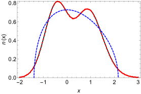
Figure 1: Thomas-Fermi (dashed) and semiclassical (dotted) approximations to the density (solid) of 2 particles in a Morse potential, $v(x)=15(e^{-x/2}-2\,e^{-x/4})$.

To begin, at energy $E$, the left ($x_{-}$) and right ($x_{+}$) classical turning points satisfy $v(x_{\pm})=E$. The action, measured from the left turning point, is

$$S(x,E)=\int^{x}_{x_{-}(E)}dx\,p(x,E)$$ (3)

where $p(x,E)=\sqrt{2m[E-v(x)]}$ is the classical momentum. The WKB quantization condition Kramers (1926); Berry and Mount (1972); Child (1991) is then

$$S\left[x_{+}(E_{j}),E_{j}\right]=\pi\hbar\left(j+\frac{1}{2}\right),~{}~{}~{}~{}~{}j\in\mathbb{N}.$$ (4)

The accuracy of WKB quantized energies generally improve as either $j$ or $m$ grows, $\hbar$ shrinks, or the potential is stretched such that its rate of change becomes smaller Child (1991); Bender and Orszag (1978). But the WKB wavefunction is singular in the turning point region Jeffreys (1925); Wentzel (1926); Brillouin (1926); Kramers (1926); Child (1991). Langer Langer (1937) obtained a semiclassical wavefunction for the case where turning points are simple zeroes of the momentum:

$$\phi_{j}(x)=\sqrt{\frac{2m\omega_{j}}{p_{j}(x)}}\,z_{j}^{1/4}(x)\,\operatorname{Ai}\left[-z_{j}(x)\right],$$ (5)

where $\omega_{j}=\hbar^{-1}\partial E_{\lambda}/\partial\lambda|_{\lambda=j}$ is the frequency of the corresponding classical orbit, and $z_{j}=\left[3S_{j}(x)/2\hbar\right]^{2/3}$. In a classically-forbidden region, $-p(x)=-i|p(x)|=e^{3i\pi/2}|p(x)|$, ensuring continuity through the turning point. The Langer solution can also be used for problems with two turning points Miller (1968). In this work we match Langer functions from each turning point at the mid-phase point $x_{m}^{j}$ where $S_{j}(x_{m}^{j})=\hbar(j+1/2)\pi/2$. This procedure ensures continuity everywhere.

Our task is to use Langer orbitals to find the asymptotic behavior of the density of $N$ occupied orbitals,

$$n(x)=\sum_{j=0}^{N-1}|\phi_{j}(x)|^{2}.$$ (6)

We use the Poisson summation formula:

$$\sum_{j=0}^{N-1}f_{j}=\sum_{k=-\infty}^{\infty}\int_{-1/2}^{N-1/2}d\lambda\,f(\lambda)e^{2\pi ik\lambda},$$ (7)

where $f(\lambda)$ is essentially any continuous function with bounded first derivatives (except for a finite number of points) that matches the $f_{j}$ when $\lambda\in\mathbb{N}$ Morse and Feshbach (1953); Berry (1966); Crowley (1979). Write

$$n(x)=n_{0}(x)+n_{1}(x),$$ (8)

where $n_{0}(x)$ is the contribution from $k=0$, and $n_{1}(x)$ is all the rest. Then, for $m=1$,

$$n_{0}(x)=2\int_{-1/2}^{N-1/2}\mathrm{d}\lambda\frac{\omega_{\lambda}\sqrt{z_{\lambda}(x)}}{p_{\lambda}(x)}\operatorname{Ai}^{2}[-z_{\lambda}(x)].$$ (9)

The lower bound of the integral corresponds to the stable fixed point of the potential well, and the upper bound defines $E_{F}$ as that obtained by solving Eq. (4)  for $j=N-1/2$, where $N$ is the number of particles in the system. Hereinafter, a subscript $F$ denotes evaluation at $E_{\scriptscriptstyle\rm F}$, and $x$ is treated as a parameter. For instance, to approximate the integral in Eq. 9 we employ the transformation $\lambda\rightarrow p_{\lambda}(x)$. Integrating by parts, using the Airy differential equation Vallee and Soares (2004), changing variables, and neglecting higher-order terms from the lower-bound of the integral in Eq. 9, we find:

$$n_{0}(x)\sim\hbar^{-1}p_{\scriptscriptstyle\rm F}(x)\,g_{+}[z_{\scriptscriptstyle\rm F}(x)]+\int_{z_{-1/2}(x)}^{z_{F}(x)}\mathrm{d}z\,{\sqrt{z}}\frac{\partial f}{\partial z}g_{-}(z),$$ (10)

where

$$g_{\pm}(z)=z^{1/2}\,\operatorname{Ai}^{2}(-z)\pm z^{-1/2}\,{\operatorname{Ai}^{\prime}}^{2}(-z)$$ (11)

$f(z)=p(z)/{\sqrt{z}}$, and $\operatorname{Ai}^{\prime}(z)=\mathrm{d}\operatorname{Ai}(z)/\mathrm{d}z$.

Eq. (10) is useful for the extraction of the dominant terms in an asymptotic expansion for $n_{0}(x)$. As $N$ grows, the coefficients $\sqrt{z}\partial f/\partial z$ become ever more slowly-varying functions of the energy. Integrating by parts, ignoring the remaining higher-order contribution, and using

$$\frac{\partial f}{\partial z}\bigg{|}_{E_{F},x}=\frac{\omega_{\scriptscriptstyle\rm F}}{p_{\scriptscriptstyle\rm F}(x)\alpha_{\scriptscriptstyle\rm F}(x)}-\frac{p_{\scriptscriptstyle\rm F}(x)}{2\hbar z_{\scriptscriptstyle\rm F}^{3/2}(x)},$$ (12)

where $\alpha_{F}(x)=$ $\sqrt{z_{F}(x)}\hbar^{-1}~{}\partial z_{\lambda}(x)/\partial\lambda|_{\lambda=N-1/2}$ (e.g, $=\omega_{F}\int_{x_{-}(E_{F})}^{x}\mathrm{d}x^{\prime}/p(x^{\prime})$ for $x_{-}(E_{F})<x<x_{m}$). We find

$$n_{0}(x)\sim\hbar^{-1}p_{F}(x)g_{+}[z_{\scriptscriptstyle\rm F}(x)]+\frac{\partial f}{\partial z}\bigg{|}_{E_{F},x}\ A_{0}[z_{\scriptscriptstyle\rm F}(x)],$$ (13)

where $A_{0}(z)=\operatorname{Ai}(-z)\operatorname{Ai}^{\prime}(-z)$.

To evaluate the $k\neq 0$ components of Eq. 7, we use the integral representation of $\operatorname{Ai}^{2}(-z)$ Vallee and Soares (2004) and change variable to $G_{\lambda}(x)=2\pi\,k\,\lambda-z_{\lambda}(x)\ t$,

$$n_{1}(x)=2\sum_{k=-\infty}^{\infty^{\prime}}\small{\lim_{T\rightarrow\infty}}\int_{-T}^{T}\mathrm{d}t~{}\kappa(t)\int_{G_{-1/2}}^{G_{F}}\frac{\mathrm{d}G_{\lambda}~{}\omega_{\lambda}\sqrt{z_{\lambda}}}{p_{\lambda}\frac{\partial G_{\lambda}}{\partial\lambda}}e^{iG_{\lambda}},$$ (14)

where the sum is over all $k\neq 0$, and $\kappa=i\exp(it^{3}/12)/(4{\sqrt{i\pi^{3}t}})$. Integration by parts assuming negligible contributions from the lower bound yields, to leading order in $\hbar$ (or $1/N$):

$$n_{1}(x)\sim 2\frac{\omega_{F}\sqrt{z_{F}}}{p_{F}}\sum_{k=-\infty}^{\infty^{\prime}}(-1)^{k}\lim_{T\rightarrow\infty}\int_{-T}^{T}\mathrm{d}t\frac{\kappa(t)e^{-iz_{F}t}}{2\pi k-y_{F}t},$$ (15)

where $y_{F}=\alpha_{\scriptscriptstyle\rm F}/{\sqrt{z_{\scriptscriptstyle\rm F}}}$. The factor $(2\pi k-y_{F}t)^{-1}$ may be expressed as geometric series in $ty_{F}/(2\pi k)$, with a radius of convergence $R_{F}=\left|2\pi k/y_{F}\right|$, which becomes arbitrarily large as $|k|$ becomes greater and $|y_{F}|$ becomes smaller. This condition is generally fulfilled when $v(x)$ has an infinite number of bound states, or if the semiclassical limit is approached by stretching the coordinateElliott et al. (2008); Cangi et al. (2010); Lieb (1981). Assuming any errors introduced by this sequence of operations vanish in the semiclassical limit the integrals required for the evaluation of $n_{1}(x)$ can be performed Vallee and Soares (2004) and the results summed to give an asymptotic expansion for $n_{1}(x)$ in terms of $A_{0}[z]=\operatorname{Ai}[-z]Ai^{\prime}[-z]$, $A_{1}[z]=\operatorname{Ai}^{2}[-z]$ and $A_{2}[z]=\operatorname{Ai}^{{}^{\prime}2}[-z]$:

$$n_{1}(x)\sim\frac{\omega_{F}}{p_{F}}\sum_{p=0}^{2}\sum_{j=0}^{\infty}\left(-z_{F}\right)^{-3j-p}\xi_{3j+p}(\alpha_{F})A_{p}[z_{F}],$$ (16)

where $\{\xi_{j}(\alpha_{F})\}$ correspond to different power series in $\alpha_{F}(x)$, e.g.,

$$\xi_{0}(\alpha)=\sum_{k=1}^{\infty}\frac{(-1)^{k-1}2\left(2^{2k-1}-1\right)B_{2k}}{(2k)!}\alpha^{2k-1},$$ (17)

where $B_{2k}$ denotes the $2k$th Bernoulli number Abramowitz and Stegun (1965). Eq. 17 may also be expressed as $-1/\alpha+\text{csc}~{}\alpha$. However, to extract the leading term of $n_{1}(x)$, only the term with highest-power in $z_{F}(x)$ needs to be considered, yielding

$$n_{1}(x)\sim\frac{\omega_{F}}{p_{F}(x)}\left[\text{csc}\left[\alpha_{F}(x)\right]-\frac{1}{\alpha_{F}(x)}\right]A_{0}[z_{F}(x)].$$ (18)

The sum of Eqs. 13 and 18 yields Eq. (2). The relative orders of each term in $\hbar$ only become explicit after accounting for the $z_{F}(x)$ dependence, which changes in different regions (see below). For instance, while the rightmost term in Eq. 2 has a multiplying factor of $\hbar^{-1}$, it is canceled by the $\hbar^{-1}$ in $z_{F}^{-3/2}(x)$. Equation 2 also illustrates the vital balance between the asymptotic expansions constructed for $n_{0}(x)$ and $n_{1}(x)$. The former (see Eq. 13) contains the pole $\alpha_{F}^{-1}$ of the Laurent series for $\text{csc}\left(\alpha_{F}\right)$ about $\alpha_{F}=0$ (turning point), whereas Eq. 17 contains all remaining terms of the series.

Further, if we choose

$$t(x)=\sum_{j=0}^{N-1}p_{j}^{2}(x)|\phi_{j}(x)|^{2}/2,$$ (19)

similar steps produce

$$t^{\rm sc}(x)=\frac{p_{\scriptscriptstyle\rm F}^{2}(x)}{6}\,n^{\rm sc}(x)+\frac{p_{F}(x)\omega_{F}}{3\text{sin}\alpha_{F}(x)}A_{0}[z_{F}(x)].$$ (20)

Eqs. (2) and (20) define closed form global uniform semiclassical approximations to $n(x)$ and $t(x)$ which are asymptotically exact as $\hbar\rightarrow 0$ or $N\to\infty$.

These approximations simplify in different regions.

Classically-allowed: For $z_{F}(x)>>1$, the asymptotic form of the Airy function applies, leading to

$$n^{\rm sc}(x)\to\frac{p_{F}(x)}{\hbar\pi}-\frac{\omega_{F}\cos\left[2S_{F}(x)/\hbar\right]}{2\pi p_{F}(x)\sin\alpha_{F}(x)},$$ (21)

(simplifying Eq. (3.36) of Ref. Kohn and Sham (1965); see also Lee and Light (1975)). The dominant smooth term arises from the direct short-time classical orbitBerry and Mount (1972); Light and Yuan (1973). The oscillatory contributions arise from single- (in $n_{0}(x)$) and multiple- (in $n_{1}(x)$) reflections from each turning point Berry and Mount (1972); Light and Yuan (1973); Lee and Light (1975); Roccia and Brack (2008).

Evanescent: For $x$ far outside the classically allowed region for the density, $-z_{F}(x)>>1$, and

$$n^{\rm sc}(x)\to\left[\frac{p_{F}(x)}{3S_{F}(x)}-\frac{\omega_{F}}{p_{F}(x)\sin\alpha_{F}(x)}\right]\frac{e^{-2|S_{F}(x)|/\hbar}}{4\pi},$$ (22)

generalizing the approximation of Ref. Kohn and Sham (1965). Similarly,

$$t^{\rm sc}(x)\to\left[\frac{p_{F}^{3}(x)}{3S_{F}(x)}-\frac{3\omega_{F}p_{F}(x)}{\text{sin}\alpha_{F}(x)}\right]\frac{e^{-2|S_{F}(x)|/\hbar}}{24\pi},$$ (23)

Turning point: At a Fermi energy turning point $x_{0}$, where $v^{\prime}(x_{0})\neq 0$, the leading term in the density is known:

$$n^{\rm sc}(x_{0})=c_{0}\hbar^{-2/3}|dv/dx|^{1/3},$$ (24)

where $c_{0}=(2/9)^{1/3}/\Gamma^{2}(1/3)$ Kohn and Sham (1965). In addition,

$$t^{\rm sc}(x_{0})=-d_{0}|dv/dx|$$ (25)

where $d_{0}=1/[9\Gamma(2/3)\Gamma(1/3)]$.

The present development unifies all earlier partial resultsKohn and Sham (1965); Lee and Light (1975); Roccia and Brack (2008); Cangi et al. (2010). In Fig. 1, we showed how accurate the semiclassical density is in a Morse potential that supports 21 levels. In Fig. 2, we plot the density error for 2 and 8 particles. The cusp in the center is at the mid-phase point $x_{m}^{N-1/2}$ where the left- meets the right-turning point solution.

To quantify, we define a measure of density difference as

$$\eta=\frac{1}{N}\int_{-\infty}^{\infty}dx\,|n^{sc}(x)-n(x)|,$$ (26)

which only vanishes when two densities are identical pointwise, and remains comparable in magnitude to the pointwise difference. In Fig. 3, we plot this error measure for the uniform approximation for the number density in Eq. 2 and for the TF density (Eq.1) as a function of $N$. As $N$ grows, $\eta$ shrinks until levels close to the unstable point of the well are included.

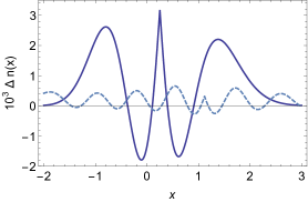
Figure 2: Error in semiclassical density for $N=2$ (solid), and $N=8$ (dashed) in the Morse potential of Fig. 1.

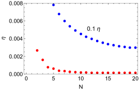
Figure 3: Integrated measure of error (Eq. 26) in TF density multiplied by 0.1 (top) and semiclassical uniform approximation (bottom) for the Morse potential of Fig. 1.

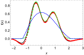
Figure 4: Thomas-Fermi (dashed), uniform semiclassical (dotted) and exact (solid) kinetic energy density for 2 particles in the Morse potential of Fig. 1. The value of $\pi^{2}[n^{\rm sc}(x)]^{3}/6$ is also shown (dot-dashed).

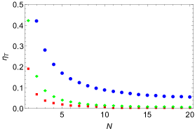
Figure 5: Error (see text) in kinetic energy densities in the Morse potential of Fig. 1 with the semiclassical uniform approximation (squares), Thomas-Fermi theory (dots) and $t^{\text{loc}}[n^{\text{sc}}]$ (rhombs).

In Fig. 4, we plot $t(x)$. The TF result clearly misses the oscillations and everything beyond the turning points. The exact $t(x)$ becomes negative near the turning points and this effect is well captured by the uniform semiclassical approximation. Brack et al. Roccia et al. (2010) noted that $t^{\text{loc}}[n]=\pi^{2}n^{3}/6$ evaluated on the exact density can yield an accurate approximation, but only in the classically-allowed region. The improvement of the uniform approximation with increasing $N$ is reflected in Fig. 5, in which $\eta_{T}$ is defined analogously to Eq. (27) except with the exact $T$ in the denominator. We find qualitatively similar results for several other systems including those with uncountable (Rosen-MorseRosen and Morse (1932) potential) and countable spectra (simple harmonic oscillator and quartic oscillator). Longer accounts of the derivation, performance, and relation to DFT are in preparation.

Eq. (2) cannot be applied to three-dimensions, Coulomb potentials, multi-center problems or interacting particles, whereas TF theory can be applied to almost any fermionic problem. But Eq. (2) strongly suggests corrections to TF exist (even if they can only be evaluated numerically), are extremely accurate, and must reduce to Eq. (2) where applicable. Without Eq. (2), we would have no reason to search for them. Now we have.

We acknowledge NSF Grant NO. CHE-1112442. We thank Michael Berry for useful discussions.

References

- Brack and Bhaduri (2003) M. Brack and R.K. Bhaduri, Semiclassical Physics, Frontiers in physics (Westview, 2003).
- Child (1991) M. S. Child, Semiclassical Mechanics with Molecular Applications (Clarendon Press, Oxford, UK, 1991).
- Griffiths (2005) D. J. Griffiths, Introduction to Quantum Mechanics (Pearson Prentice Hall, Upper Saddle River, 2005).
- Thomas (1927) L. H. Thomas, “The calculation of atomic fields,” Math. Proc. Camb. Phil. Soc. 23, 542–548 (1927).
- Fermi (1927) E. Fermi, “Un metodo statistico per la determinazione di alcune proprieta dell’atomo,” Rend. Accad. Naz. Lincei 6, 602 (1927).
- Schrodinger (1926) E. Schrodinger, “Quantisierung als eigenwertproblem,” Annalen der Physik 384, 361–376 (1926).
- Spruch (1991) L. Spruch, “Pedagogic notes on thomas-fermi theory (and on some improvements): atoms, stars, and the stability of bulk matter,” Rev. Mod. Phys. 63, 151 (1991).
- Hohenberg and Kohn (1964) P. Hohenberg and W. Kohn, “Inhomogeneous electron gas,” Phys. Rev. 136, B864–B871 (1964).
- Lieb and Simon (1973) Elliott H. Lieb and Barry Simon, “Thomas-fermi theory revisited,” Phys. Rev. Lett. 31, 681–683 (1973).
- Lieb (1981) E. H. Lieb, “Thomas-fermi and related theories of atoms and molecules,” Rev. Mod. Phys. 53, 603–641 (1981).
- Alfred (1961) L. C. R. Alfred, “Quantum-corrected statistical method for many-particle systems: The density matrix,” Phys. Rev. 121, 1275–1282 (1961).
- Stephen and Zalewski (1962) M. J. Stephen and K. Zalewski, “On the classical approximation involved in the thomas-fermi theory,” Proceedings of the Royal Society of London. Series A. Mathematical and Physical Sciences 270, 435–442 (1962).
- Payne (1963) H. Payne, “Nature of the quantum corrections to the statistical model,” Phys. Rev. 132, 2544–2546 (1963).
- Payne (1964) H. Payne, “Approximation of the dirac density matrix,” The Journal of Chemical Physics 41, 3650–3651 (1964).
- Kohn and Sham (1965) W. Kohn and L. J. Sham, “Quantum density oscillations in an inhomogeneous electron gas,” Phys. Rev. 137, A1697–A1705 (1965).
- Grover (1966) R. Grover, “Asymptotic expansions of the dirac density matrix,” Journal of Mathematical Physics 7, 2178–2186 (1966).
- Balazs and Jr. (1973) N.L Balazs and G.G Zipfel Jr., “Quantum oscillations in the semiclassical fermion ÎŒ-space density,” Annals of Physics 77, 139 – 156 (1973).
- Light and Yuan (1973) J. C. Light and J. M. Yuan, “Quantum path integrals and reduced fermion density matrices: One-dimensional noninteracting systems,” The Journal of Chemical Physics 58, 660–671 (1973).
- Lee and Light (1975) S. Y. Lee and J. C. Light, “Uniform semiclassical approximation to the electron density distribution,” The Journal of Chemical Physics 63, 5274–5282 (1975).
- Englert (1988) B.-G. Englert, “Semiclassical theory of atoms,” Lec. Notes Phys. 300 (1988).
- Elliott et al. (2008) P. Elliott, D. Lee, A. Cangi, and K. Burke, “Semiclassical origins of density functionals,” Phys. Rev. Lett. 100, 256406 (2008).
- Cangi et al. (2013) A. Cangi, E. K. U. Gross, and K. Burke, “Potential functionals versus density functionals,” Phys. Rev. A 88, 062505 (2013).
- Morse and Feshbach (1953) P. M. Morse and H. Feshbach, Methods of Theoretical Physics (McGraw-Hill Science/Engineering/Math, 1953).
- Crowley (1979) B. J. B. Crowley, “Some generalisations of the poisson summation formula,” Journal of Physics A: Mathematical and General 12, 1951 (1979).
- Berry and Mount (1972) M. V. Berry and K. E. Mount, “Semiclassical approximations in wave mechanics,” Reports on Progress in Physics 35, 315 (1972).
- Berry and Tabor (1976) M. V. Berry and M. Tabor, “Closed orbits and the regular bound spectrum,” Proceedings of the Royal Society of London. Series A, Mathematical and Physical Sciences 349, pp. 101–123 (1976).
- Kramers (1926) H.A. Kramers, “Wellenmechanik und halbzählige quantisierung,” Z. Phys. 39, 828 (1926).
- Bender and Orszag (1978) C. M. Bender and S. A. Orszag, Advanced Mathematical Methods for Scientists and Engineers, New York: McGraw-Hill, 1978 (McGraw-Hill, New York, NY, 1978).
- Jeffreys (1925) H. Jeffreys, “On certain approximate solutions of lineae differential equations of the second order,” Proceedings of the London Mathematical Society s2-23, 428–436 (1925).
- Wentzel (1926) G. Wentzel, “Eine verallgemeinerung der quantenbedingungen für die zwecke der wellenmechanik,” Z. Phys. 38, 518 (1926).
- Brillouin (1926) L. Brillouin, “La mecanique ondulatoire de schrödinger: une methode generale de resolution par approximations successives,” Comptes Rendus de l’Academie de Sciences 183, 24 (1926).
- Langer (1937) R. E. Langer, “On the connection formulas and the solutions of the wave equation,” Phys. Rev. 51, 669–676 (1937).
- Miller (1968) William H. Miller, “Uniform semiclassical approximations for elastic scattering and eigenvalue problems,” The Journal of Chemical Physics 48, 464–467 (1968).
- Berry (1966) M. V. Berry, “Uniform approximation for potential scattering involving a rainbow,” Proceedings of the Physical Society 89, 479 (1966).
- Vallee and Soares (2004) Olivier Vallee and Manuel Soares, Airy Functions and Applications to Physics (Imperial College Press, London, 2004).
- Cangi et al. (2010) A. Cangi, D. Lee, P. Elliott, and K. Burke, “Leading corrections to local approximations,” Phys. Rev. B 81, 235128 (2010).
- Abramowitz and Stegun (1965) M. Abramowitz and I.A. Stegun, Handbook of Mathematical Functions: With Formulas, Graphs, and Mathematical Tables, Applied mathematics series (Dover Publications, 1965).
- Roccia and Brack (2008) J. Roccia and M. Brack, “Closed-orbit theory of spatial density oscillations in finite fermion systems,” Phys. Rev. Lett. 100, 200408 (2008).
- Roccia et al. (2010) J. Roccia, M. Brack, and A. Koch, “Semiclassical theory for spatial density oscillations in fermionic systems,” Phys. Rev. E 81, 011118 (2010).
- Rosen and Morse (1932) N. Rosen and P. M. Morse, “On the vibrations of polyatomic molecules,” Phys. Rev. 42, 210–217 (1932).