Sampling artifact in volume weighted velocity measurement.— II. Detection in simulations and comparison with theoretical modelling

Abstract

Measuring the volume weighted velocity power spectrum suffers from a severe systematic error due to imperfect sampling of the velocity field from the inhomogeneous distribution of dark matter particles/halos in simulations or galaxies with velocity measurement. This “sampling artifact” depends on both the mean particle number density $\bar{n}_{P}$ and the intrinsic large scale structure (LSS) fluctuation in the particle distribution. (1) We report robust detection of this sampling artifact in N-body simulations. It causes $\sim 12\%$ underestimation of the velocity power spectrum at $k=0.1h/{\rm Mpc}$ for samples with $\bar{n}_{P}=6\times 10^{-3}({\rm Mpc}/h)^{-3}$. This systematic underestimation increases with decreasing $\bar{n}_{P}$ and increasing $k$. Its dependence on the intrinsic LSS fluctuations is also robustly detected. (2) All of these findings are expected based upon our theoretical modelling in paper I Zhang et al. (2015). In particular, the leading order theoretical approximation agrees quantitatively well with the simulation result for $\bar{n}_{P}\gtrsim 6\times 10^{-4}({\rm Mpc}/h)^{-3}$. Furthermore, we provide an ansatz to take high order terms into account. It improves the model accuracy to $\lesssim 1\%$ at $k\lesssim 0.1h/{\rm Mpc}$ over 3 orders of magnitude in $\bar{n}_{P}$ and over typical LSS clustering from $z=0$ to $z=2$. (3) The sampling artifact is determined by the deflection ${\bf D}$ field, which is straightforwardly available in both simulations and data of galaxy velocity. Hence the sampling artifact in the velocity power spectrum measurement can be self-calibrated within our framework. By applying such self-calibration in simulations, it is promising to determine the real large scale velocity bias of $10^{13}M_{\odot}$ halos with $\sim 1\%$ accuracy, and that of lower mass halos with better accuracy. (4) In contrast to suppressing the velocity power spectrum at large scale, the sampling artifact causes an overestimation of the velocity dispersion. We prove that correlation between the signal field (${\bf v}$) and the sampling field (${\bf D}$) is a major cause. This complexity, among others, shall be carefully investigated to further improve understanding of the sampling artifact.

I Introduction

Peculiar velocity is a powerful probe of cosmology, with increasing importance. A statistics of particular importance to peculiar velocity cosmology is the volume weighted velocity power spectrum. Unlike the density weighted velocity, it is free of uncertainties in galaxy density bias, which is hard to predict from first principle. So the volume weighted velocity is desired for the purpose of cosmology. However it is challenging to measure it accurately, both in simulations and in observations with galaxy velocity measurement. The measurement suffers from the sampling artifact Bernardeau and van de Weygaert (1996), which arises from the fact that we often cannot fairly sample the volume weighted velocity field. For example, the distribution of galaxies with velocity measurement through distance indicators (e.g. Watkins and Feldman (2014); Johnson et al. (2014)) is not only sparse but also spatially clustered. Even worse, their spatial distribution is correlated with the velocity field that we try to measure, due to the underlying correlation between the large scale structure (LSS) and velocity. Hence the sampling of volume weighted velocity field is biased.

This sampling artifact has three-fold impacts on cosmology. (1) The velocity power spectrum (and higher order statistics) measured through galaxy velocity data is systematically biased by this sampling artifact. (2) The same sampling artifact also exists in measuring the velocity power spectrum of dark matter (DM) particles/halos in N-body simulations. This can systematically bias our theoretical understanding of the velocity field, for example the physical velocity bias of halos. (3) A biased theoretical understanding can lead to biased cosmological constraints, even if the velocity measurements themselves, such as that inferred from redshift space distortion, are free of the sampling artifact. Hence this sampling artifact is entangled in key ingredients of peculiar velocity cosmology. It is a significant source of systematic errors, which we should investigate intensively. Throughout this paper, we will focus on its impact on peculiar velocity power spectrum. Unless otherwise specified, we always refer to the peculiar velocity power spectrum as the volume weighted one.

In Zhang et al. (2015) (hereafter paper I) we present a theoretical modelling of the sampling artifact in measuring the volume weighted velocity power spectrum. The present paper (paper II) focuses on its numerical verification in order to improve our understanding of the sampling artifact. In Zheng et al. (2014) we will apply this improved understanding to correct the sampling artifact in the halo/galaxy velocity field and robustly measure the halo velocity bias.

In paper I we find that the sampling artifact is fully captured by the “deflection” field ${\bf D}$. ${\bf D}$ is the spatial separation vector pointing from a particle used for velocity assignment to a grid point that the velocity is assigned with this particle. Within this framework, we predict that the sampling artifact causes underestimation in the velocity power spectrum at large scale. Furthermore, this systematic underestimation increases with decreasing particle number density $\bar{n}_{P}$ and increasing $k$. With a number of simplifications we are able to derive analytical expressions for this underestimation. We estimate that it is significant, $\sim 10$% at $k=0.1h/{\rm Mpc}$, for $\bar{n}_{P}=10^{-3}({\rm Mpc}/h)^{-3}$. Without correcting it, the velocity bias of $10^{13}M_{\odot}$ halos measured in N-body simulations will be systematically underestimated by $\sim 5\%$, from its real value. This systematic underestimation/error is larger than the expected statistical error in peculiar velocity determination from redshift space distortion (RSD) by surveys like BigBOSS/MS-DESI Schlegel et al. (2011), Euclid and SKA . Furthermore, it is of comparable size and sign as the physical velocity bias ($b_{v}<1$) predicted through proto-halo statistics Bardeen et al. (1986); Desjacques (2008); Desjacques and Sheth (2010). Hence it could mislead the theory comparison, if not corrected. Therefore the sampling artifact is clearly a severe obstacle to theoretical understanding and observational application of peculiar velocity.

The existence of sampling artifact in the volume weighted velocity power spectrum has been realized in simulations Zheng et al. (2013); Jennings et al. (2014); Zheng et al. (2014), for both the DM and halo velocity fields. These works found that its impact increases with decreasing number density. This behavior can be used to diagnose the sampling artifact Zheng et al. (2013); Jennings et al. (2014). For example, by comparing the velocity power spectrum $P_{v}$ of two halo populations at equal volume density, difference in $P_{v}$ is significantly suppressed Jennings et al. (2014), manifesting the existence of sampling artifact. One complexity is that the sampling artifact also depends on the spatial clustering of halos/DM particles Zhang et al. (2015). Hence two halo populations of identical number density but different mass do not have identical sampling artifact, due to difference in their spatial clustering. This complexity makes clean separation of sampling artifact from a possible halo velocity bias highly nontrivial, since the halo number density, density bias and velocity bias can all vary with the halo mass. In contrast, since all randomly selected DM populations at the same redshift have statiatically identical spatial clustering, the sampling artifact can be robustly isolated, as done in Zheng et al. (2013). The present paper extends its numerical verification and quantification to much wider range of DM density and redshift, and is better theory motivated and backed up Zhang et al. (2015). By comparing with the sampling artifact of DM populations with various number density at various redshifts, we hope to develop generic theoretical modelling of the sampling artifact, applicable to a wide range of particle number density and spatial clustering. We can then robustly predict the sampling artifact in halo velocity and circumvent the difficulty of directly measuring it.

Our paper is organized as follows. In §II we report the detection of sampling artifact in the volume weighted velocity power spectrum measurement, including its dependence on $\bar{n}_{P}$ and redshift/spatical clustering. In §III we compare it with the theoretical modelling developed in paper I Zhang et al. (2015). We also propose an ansatz to further improve its accuracy. In §IV we discuss the possibility to self-calibrate this sampling artifact . The appendix §A & §C discuss more aspects of the sampling artifact, other than the suppression of power discussed in the main text. These aspects are important and deserve further investigation.

II Detection of the sampling artifact in simulations

For brevity, we will focus on the gradient part of the velocity ${\bf v}_{E}$ ($\nabla\times{\bf v}_{E}=0$), which contains most of cosmological information. Given a sample of simulation particles/halos/galaxies with velocity information, we can measure the volume weighted velocity power spectrum $\hat{P}_{E}(k)$. The hat $\hat{}$ denotes the measured quantity, instead of the one without measurement error (the sampling artifact to be specific). The measurement can be done using one’s favorite velocity assignment method, such as the ones based on Voronoi and Delaunay tessellations Bernardeau and van de Weygaert (1996). Throughout this paper, we restrict to the NP (Nearest Particle) method Zheng et al. (2013). As discussed in paper I, sampling artifacts in other velocity assignment methods are similar. So results on the sampling artifact in the NP method also provide useful reference for that in other methods.

II.1 The method to detect the sampling artifact

Without knowing the correct velocity power spectrum $P_{E}(k)$, we are not able to carry out direct comparison with $\hat{P}_{E}(k)$ to measure the sampling artifact. This problem is circumvented in Zheng et al. (2013). We randomly select a fraction $f$ of simulation DM (dark matter) particles to construct a sub-sample. We then apply the same analysis to this sub-sample to measure the velocity power spectrum, which we denote as $\hat{P}_{E}(k|f)$. So the measurement using the whole sample is $\hat{P}_{E}(k|f=1)$. If there is no sampling artifact, we should have $\hat{P}_{E}(k|f)=\hat{P}_{E}(k|f=1)$, since simulation particles in the sub-sample are selected randomly from the full sample without prejudice . Hence the ratio

$$\eta(k|f)\equiv\frac{\hat{P}_{E}(k|f)}{\hat{P}_{E}(k|f=1)}$$ (1)

measures the sampling artifact . In another word, if $\eta\neq 1$, the sampling artifact exists.

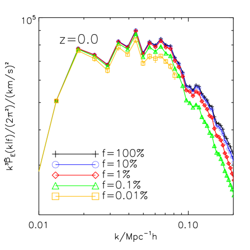
Figure 1: The measured velocity power spectra of DM samples at $z=0$ with various number density. To highlight the sampling artifact, we randomly select a fraction $f$ of DM particles to construct DM sub-samples and then measure the corresponding velocity power spectrum. Without the sampling artifact, the measured power spectrum $\hat{P}_{E}(k|f)$ should be identical to that of the full sample $\hat{P}_{E}(k|f=100\%)$. However, in simulations we find a systematic suppression, which increases with decreasing number density and increasing $k$. The error bars of sub-samples are estimated using $10$ sub-samples of identical $f$. For the J1200 simulation specification, the mean particle number density $\bar{n}_{P}=0.62f({\rm Mpc}/h)^{-3}$.

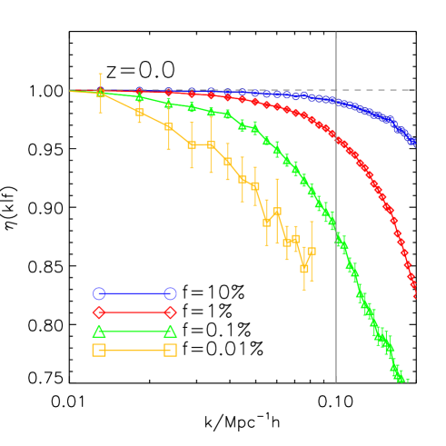
Figure 2: $\eta(k|f)\equiv\hat{P}_{E}(k|f)/\hat{P}_{E}(k|f=1)$ at $z=0$. $\eta<1$ means systematic underestimation of the velocity power spectrum, caused by the sampling artifact. This systematic underestimation can be severe, even at relatively large scale $k=0.1h/{\rm Mpc}$, increasing from $1\%$ for $f=10\%$) ($\bar{n}_{P}=6.2\times 10^{-2}({\rm Mpc}/h)^{-3}$) to $\sim 12\%$ $f=0.1\%$ ($\bar{n}_{P}=6.2\times 10^{-4}({\rm Mpc}/h)^{-3}$).

This method of measuring sampling artifact can be applied to both DM particles and halos. But due to low number density of halos, the measurement of $\eta$ is noisy. So we will focus on $\eta(k|f)$ of DM particles. Nevertheless, we expect the results to be general, not limited to the case of DM particles, for two reasons. (1) As addressed in paper I, the sampling artifact is determined by the deflection field ${\bf D}$, which is determined both by $\bar{n}_{P}$ and the intrinsic LSS fluctuation in the particle distribution. By analyzing DM sub-samples with different $f$ at different simulation snapshots, we cover not only a large parameter space in $\bar{n}_{P}$, but also different intrinsic LSS clustering. (2) We also use these results on DM particles to test and improve our theoretical understanding. Our theoretical modelling does not make assumption on whether the sample dealt with is DM particles or DM halos. Hence we expect that, as long as the theoretical modelling works for DM particles, it should work for halos as well.

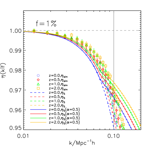
Figure 3: $\eta(k|f=1\%)$ at $z=0.0$, $0.5$, $1.0$ and $2.0$, in simulations (data points) and in theory (curves). $f=1\%$ corresponds to $\bar{n}_{P}=6.2\times 10^{-3}({\rm Mpc}/h)^{-3}$. $\eta$ increases with increasing redshift. This redshift dependence reflects that the sampling artifact depends not only on $\bar{n}_{P}$, but also the intrinsic LSS clustering. The dash curves are the theoretical predictions by paper I (Eq. 7). The solid lines are that of the improved ansatz Eq. III.4, which takes the spatial correlation of the ${\bf D}$ field into account. The irregularities at $k\sim 0.07h/{\rm Mpc}$ is caused by interpolation of limited data points of measured ${\bf D}$ correlation, not a fundamental feature.

II.2 The sampling artifact and its dependence on the mean number density

We analyze the same J1200 N-body simulation used in Zheng et al. (2013). It adopts the $\Lambda$CDM cosmology with $\Omega_{m}=0.268$, $\Omega_{\Lambda}=0.732$, $\sigma_{8}=0.85$, $n_{s}=1$ and $h=0.71$. It has $1024^{3}$ simulation DM particles and boxsize of $1200{\rm Mpc}/h$. It was run with a particle-particle-particle-mesh (${\rm P^{3}M}$) code Jing et al. (2007). More simulation details are presented in Zheng et al. (2013). For a sub-sample of DM particles with fraction $f$, the corresponding particle number density is $\bar{n}_{P}=0.62f({\rm Mpc}/h)^{-3}$. We use $N_{\rm grid}=256^{3}$ to analyze the velocity field and the deflection ${\bf D}$ field.

Paper I predicts $\eta<1$ at large scale. In Zheng et al. (2013) we have already found $\eta<1$, for $f=10\%$ ($\bar{n}_{P}=0.062({\rm Mpc}/h)^{-3}$). The current paper will examine the sampling artifact for wider range of number density ($6.2\times 10^{-5}$-$0.62({\rm Mpc}/h)^{-3}$), covering that of $10^{12}$-$10^{13}M_{\odot}$ halos at $z\in[0,2]$.

Fig. 1 shows $\hat{P}_{E}(k|f)$ with $f=100\%$, $10\%$, $1\%$, $0.1\%$ and $0.01\%$ at $z=0$ and Fig. 2 shows $\eta(k|f)$. In the velocity power spectrum measurement we have subtracted shot noise following Zhang et al. (2015). The alias effect Jing (2005); Pueblas and Scoccimarro (2009); Koda et al. (2013); Zhang et al. (2015) still exists. But the alias effect does not vary with $f$. So $\eta$ isolates the sampling artifact.

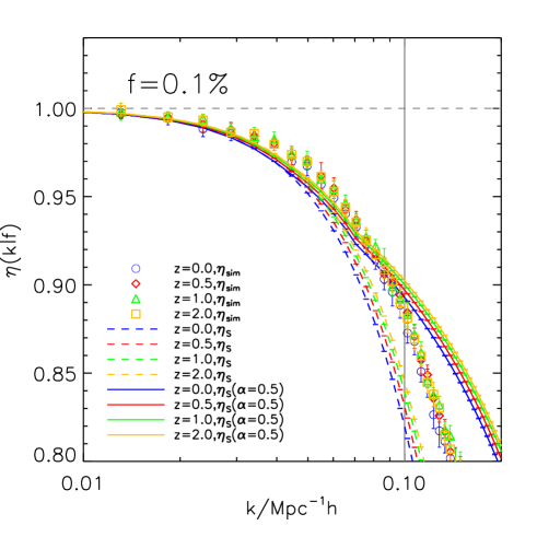
Figure 4: Same as Fig. 3, but for $f=0.1\%$ ($\bar{n}_{P}=6.2\times 10^{-4}({\rm Mpc}/h)^{-3}$). Eq. III.4 (solid curves) improves over Eq. 7 (dashed curves) from $\sim 6\%$ at $k=0.1h/{\rm Mpc}$ to $1\%$.

We detect the sampling artifact at high significance. (1) Fig. 1 & 2 clearly show systematic underestimation ($\eta<1$) of $P_{E}$, which should not exist without the sampling artifact. The result of $f=10\%$ confirms our previous finding in Zheng et al. (2013). (2) The underestimation increases with decreasing $f$ ($\bar{n}_{P}$). For $f=0.1\%$ ($\bar{n}_{P}=6.2\times 10^{-4}({\rm Mpc}/h)^{-3}$), $\eta=0.88$ at $k=0.1h/{\rm Mpc}$. This number density corresponds to $\sim 10^{13}M_{\odot}$ halos at $z=0$. This means that the velocity power spectrum of $10^{13}M_{\odot}$ halos measured without correcting the sampling artifact can be wrong by $\sim 10\%$, leading to a systematic error of $\delta b_{v}\sim-0.05$ in the halo velocity bias measurement. This is certainly a significant source of systematic error to be worried about and investigated heavily. (3) The systematic underestimation/error increases with increasing $k$. Therefore it is more challenging to understand the sampling artifact and infer cosmology at smaller scales.

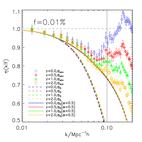
Figure 5: The same as Fig. 3 & 4, but for $f=0.01\%$ ($\bar{n}_{P}=6.2\times 10^{-5}({\rm Mpc}/h)^{-3}$). Eq. III.4 significantly improves over Eq. 7). Data points at $k\gtrsim 0.08h/{\rm Mpc}$ show anomalous behaviors. These behaviors can not be described within robust treatment of the ${\bf v}$-${\bf D}$ correlation, neglected so far in the theoretical modelling. We will discuss these complexities in the appendix §A, show the existence of the ${\bf v}$-${\bf D}$ correlation in §B, and its impact in §C .

II.3 The sampling artifact depends on the intrinsic clustering

Fig. 3, 4 & 5 show $\eta$ at redshift $z=0.0,0.5,1.0,2.0$, with $f=1\%$, $0.1\%$ and $0.01\%$ respectively. For $f=1\%$, the variation with $z$ is significant. For a fixed $f$, the DM samples at different $z$ only differ in their intrinsic LSS fluctuation. From $z=0$ to $z=2$, the clustering amplitude decreases by a factor $\sim 2.4$ in linear regime and larger factors in nonlinear regime. Hence the dependence on $z$ must be caused by the evolution in the intrinsic clustering. Therefore this redshift dependence proves that, besides $\bar{n}_{P}$, the intrinsic LSS fluctuation also affects the sampling artifact.

However, for $f=0.1\%$, the redshift dependence is already insignificant (Fig. 4). These behaviors can be interpreted as competition between two sources affecting the ${\bf D}$ field, namely Poisson fluctuation and intrinsic LSS fluctuation in the particle distribution. The former is determined by $\bar{n}_{P}$. The latter decreases towards higher redshift. The two factors both contribute and amplify the underestimation ($\eta<1$). Larger $f$ (e.g. $f=1\%$) means smaller Poisson fluctuation and hence more significant impact of LSS and redshift dependence . This point will be elaborated later in §III.

A brief summary of this section is that we have robustly detected the sampling artifact. We further identify two factors affecting the sampling artifact, $\bar{n}_{P}$ and the intrinsic LSS fluctuation. It is now the question whether the theoretical modelling can well reproduce these findings.

III Testing and improving the theoretical modelling

We now proceed to comparison between the theory and simulation, to quantify the accuracy of our model and to improve it. The ultimate goal is to develop an accurate method to correct for the sampling artifact. It can be used for two purposes. First is to accurately measure the halo velocity power spectrum and velocity bias in simulations, with the sampling artifact corrected. Such measurements at $1\%$ accuracy are needed to compare with the velocity power spectrum determined indirectly from RSD to infer the nature of dark matter, dark energy and gravity. Second, it can be applied to galaxy velocity data such as SFI++ Watkins and Feldman (2014) and 6dF Johnson et al. (2014) to measure the sampling artifact corrected velocity power spectrum.

III.1 Theoretical modelling of the sampling artifact

Here we briefly summarize our theoretical modelling of the sampling artifact in paper I Zhang et al. (2015). It targets at the NP velocity assignment method Zheng et al. (2013), but it can also be extended to methods based on various tessellation methods. In the NP method we approximate the velocity on a given grid point at position ${\bf x}$ as that of the nearest simulation particle/halo/galaxy at position ${\bf x}_{P}({\bf x})$,

$$\hat{{\bf v}}({\bf x})={\bf v}({\bf x}_{P}({\bf x}))\ .$$ (2)

Hence the sampling artifact is fully captured by the “deflection” field

$${\bf D}({\bf x})\equiv{\bf x}_{P}({\bf x})-{\bf x}\ .$$ (3)

The sampling artifact arises from ${\bf D}\neq{\bf 0}$. This distinguishes from other numerical artifacts such as the alias effect in measuring the velocity power spectrum Pueblas and Scoccimarro (2009); Koda et al. (2013).

The velocity power spectrum measured on uniform grids, after subtracting shot noise, is

$$\hat{P}_{ij}({\bf k})=\sum_{\bf q}P_{ij}({\bf q})W({\bf q},{\bf q}^{{}^{\prime}})\ .$$ (4)

Here, $\hat{P}_{ij}({\bf k})\propto\langle\hat{v}_{i}({\bf k})\hat{v}^{*}_{j}({\bf k})\rangle$. ${\bf k}$ and ${\bf q}$ are discrete Fourier modes. ${\bf q}^{{}^{\prime}}\equiv{\bf q}-{\bf k}$. The window function $W$ is

$$W({\bf q},{\bf q}^{{}^{\prime}})\equiv\frac{1}{N^{2}_{\rm grid}}\sum_{{\bf x}\neq{\bf x}^{{}^{\prime}}}S({\bf q},{\bf r})e^{i{\bf q}^{{}^{\prime}}\cdot{\bf r}}\ .$$ (5)

Here ${\bf r}\equiv{\bf x}^{{}^{\prime}}-{\bf x}$. $N_{\rm grid}$ is the total number of grid points. The window function $W({\bf q},{\bf q}^{{}^{\prime}})$ is inhomogeneous since it depends not only on ${\bf q}^{{}^{\prime}}\equiv{\bf q}-{\bf k}$, but also on ${\bf q}$. It makes the deconvolution to obtain the true velocity power spectrum more difficult.

$W({\bf q},{\bf q}^{{}^{\prime}})$ is the Fourier transform of the sampling function $S({\bf q},{\bf r})$ over ${\bf r}$. Imperfect sampling causes $S\neq 1$ and hence results in the sampling artifact. Under reasonable approximation (however refer to the appendix §A & C for caveat) we obtain

$$S({\bf q},{\bf r})=\left\langle e^{i{\bf q}\cdot({\bf D}^{{}^{\prime}}-{\bf D})}\right\rangle\ .$$ (6)

The ${\bf D}$ field is known in simulations or surveys with galaxy velocity measurement. Hence $S$ and $W$ can both be calculated. In the limit that the alias effect can be neglected, namely now ${\bf k}$ and ${\bf q}$ occupy the same space, in principle we can solve Eq. 4 to obtain the true velocity power spectrum. Unfortunately numerical evaluation of $W({\bf q},{\bf q}^{{}^{\prime}})$ is time consuming. So far we are able to reduce the calculation of all $({\bf q},{\bf q}^{{}^{\prime}})$ pairs from brute-force computation of size $O(N^{3}_{\rm grid})$ to $O(N^{2}_{\rm grid})$ (Eq. 27, paper I). But further reduction in computation is still needed to solve Eq. 4 for the true velocity power spectrum. In paper I and the current paper, we take approximations to simplify Eq. 4 for efficient evaluation of the sampling artifact.

${\bf D}\neq{\bf 0}$ leads to $S({\bf q},{\bf r})<1$. A generic prediction is that the sampling artifact causes underestimation in the velocity power spectrum at large scale . In the limit of no spatial correlation in ${\bf D}$, we are able to derive the leading order sampling artifact (Eq. 36, paper I),

$$\hat{P}^{(1)}_{E}(k)\simeq P_{E}(k)S(k)\ .$$ (7)

Here,

$$S(k)\equiv S({\bf k},{\bf r}\rightarrow\infty)=\left|\left\langle e^{i{\bf k}\cdot{\bf D}}\right\rangle\right|^{2}=e^{-\frac{1}{3}k^{2}\sigma_{D}^{2}+\cdots}\ .$$ (8)

Here, $\sigma_{D}^{2}\equiv\langle D^{2}\rangle$. The neglected terms $\cdots$ in the last expression are non-Gaussian terms in the ${\bf D}$ field.

The ${\bf D}$ field is determined by the particle distribution. So both the Poisson fluctuation and intrinsic fluctuation in the particle distribution contribute. Poisson fluctuation is completely fixed by the mean number density $\bar{n}_{P}$ ($f$). It generates (paper I)

$$\sigma_{D}^{2}\xrightarrow{\rm Poisson\ limit}0.347L_{P}^{2}\ .$$ (9)

Here $L_{P}$ is the mean separation of particles. The intrinsic clustering further increases $\sigma_{D}$.

If Poisson fluctuation in the particle number distribution dominates over the intrinsic LSS fluctuation and if the Gaussian term dominates in Eq. 8, we predict $S(k=0.1h/{\rm Mpc})=0.853$ and $\eta(k=0.1h/{\rm Mpc})|f)=0.858$ for $f=0.1\%$ ($\bar{n}_{P}=6.2\times 10^{-4}({\rm Mpc}/h)^{-3}$). meaning $15\%$ systematic underestimation of the velocity power spectrum. This prediction is already in very good agreement with numerical result ($\eta=0.87$, Fig. 4). More accurate prediction requires numerical evaluation of the ${\bf D}$ field statistics in §III.2.

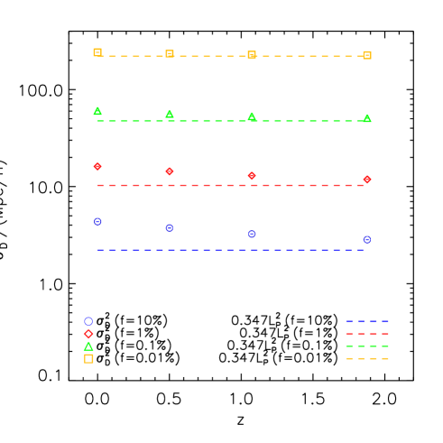
Figure 6: $\sigma_{D}^{2}\equiv\langle D^{2}\rangle$ measured in the simulation. It is the most important parameter determining the sampling artifact. It has two contributions, the Poisson fluctuation and the intrinsic LSS fluctuation in the particle distribution. A pure Poisson distribution predicts $\sigma_{D}^{2}=0.347L_{P}^{2}$ (dash lines). For $f\gtrsim 1\%$ ($\bar{n}_{P}\gtrsim 6.2\times 10^{-3}({\rm Mpc}/h)^{-3}$), the intrinsic LSS fluctuation significantly increases $\sigma_{D}$ over the Poisson limit. For smaller $f$ (lower number density) and higher redshift, Poisson fluctuation dominates.

III.2 Statistics of the ${\bf D}$ field

The ${\bf D}$ field is the key ingredient to understand the sampling artifact. In simulations, we can directly measure this field. Relevant statistics that we measure are (1) $\sigma_{D}\equiv\langle D^{2}\rangle$, (2) the non-Gaussian measures including the reduced kurtosis $K_{4}$ and the 6-th order cumulants $K_{6}$ of $D_{x}$ (equivalently $D_{y}$ and $D_{z}$), and (3) the two-point correlation function of ${\bf D}$.

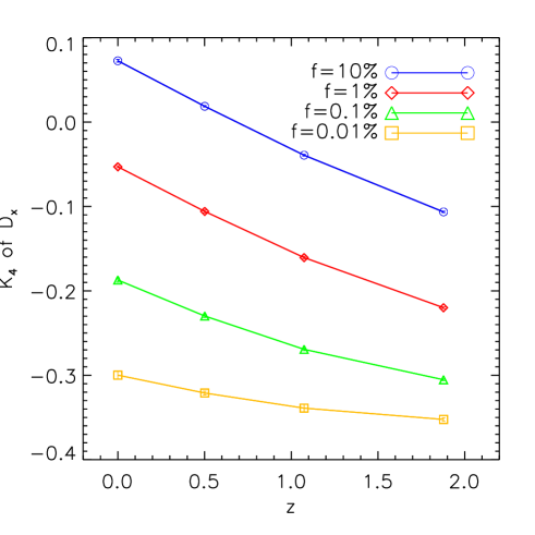
Figure 7: The reduced kurtosis $K_{4}\equiv\langle D_{x}^{4}\rangle/\langle D_{x}^{2}\rangle-3$. Due to the symmetric distribution in $D_{x}$, this is the lowest order measure of non-Gaussianity in the ${\bf D}$ field. For practically all relevant cases, the non-Gaussianity measured by $K_{4}$ is small. Nevertheless, it is non-negligible in modelling of the sampling artifact.

III.2.1 The r.m.s dispersion of the ${\bf D}$ field

$\sigma_{D}$ governs the overall amplitude of the sampling artifact. The larger $\sigma_{D}$, the stronger the suppression to the velocity power spectrum (Eq. 8). Result on $\sigma_{D}$ at $z\in[0.0,2.0]$ is shown in Fig. 6. As a reminder, both the Poisson fluctuation and the intrinsic LSS fluctuation in the particle distribution affect $\sigma_{D}$. (1) We find that the Poisson approximation (Eq. 9) is excellent for $f<0.1\%$ ($\bar{n}_{P}<6.2\times 10^{-4}({\rm Mpc}/h)^{-3}$). But for $f=0.1\%$ we begin to observe visible deviation at $z\lesssim 0.5$. For $f=10\%$ ($\bar{n}_{P}=0.062({\rm Mpc}/h)^{-3}$), $\sigma_{D}^{2}$ at $z=0$ is twice of the Poisson limit. So the contribution from intrinsic LSS fluctuation is significant. (2) $\sigma_{D}$ increases when redshift decreases. Again it manifests the role of intrinsic LSS fluctuation. It enlarges $\sigma_{D}$. When it grows with decreasing redshift, it causes $\sigma_{D}$ to increase.

To understand the competition between the Poisson fluctuation and intrinsic LSS fluctuation, we estimate the r.m.s density fluctuation generated by the two over the grid size $L_{\rm grid}=4{\rm Mpc}/h$. For Poisson fluctuation, it is $\delta_{N}=(4^{3}f)^{-1/2}=3.95(f/0.1\%)^{-1/2}$. The intrinsic linear LSS density fluctuation is $\delta_{I}\sim 1.7D(z)$ at $z\gg 1$ at such scale. So it is subdominant to $\delta_{N}$. Here $D(z)$ is the linear density growth factor. However, due to the faster growth caused by the nonlinear evolution, $\delta_{I}(z=0)\simeq\delta_{P}(f=0.1\%)$. We can then draw a general conclusion that none of them overwhelms the other for $f\sim 0.1\%$. It is for this reason $\sigma_{D}$ shows visible redshift evolution for $f=0.1\%$. It also explains why the redshift evolution becomes significant for $f\gtrsim 1\%$.

We also find that the contribution from the Poisson fluctuation to $\sigma_{D}$ is larger than its contribution to the overall fluctuation in the particle number distribution. For example, when $f=100\%$, $\delta_{N}\ll\delta_{I}$ at all relevant redshifts. Nevertheless, we still find significant contribution to $\sigma_{D}$ from the Poisson fluctuation. The Poisson fluctuation scales as $\delta_{N}\propto k^{2}$. The intrinsic LSS fluctuation scales as $\delta_{I}\propto k^{(n_{\rm eff}+3)/2}$. When $k\gg k_{\rm NL}$, $n_{\rm eff}\rightarrow-3$. Hence towards smaller scales, Poisson fluctuation increases with respect to the intrinsic LSS fluctuation. We speculate that the ${\bf D}$ field is more sensitive to smaller scale density fluctuations.

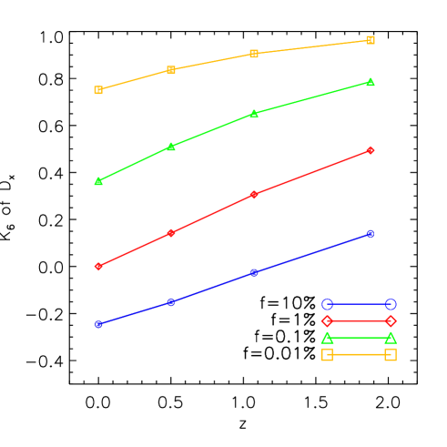
Figure 8: The reduced 6-th order cumulant $K_{6}$. The measured non-Gaussianity is insignificant. However, it is still non-negligible in modelling the sampling artifact.

III.2.2 Non-Gaussianities in the ${\bf D}$ field

Eq. 8 tells us that non-Gaussian terms also contribute to $S(k)$ and hence to the sampling artifact. For this reason we also measure the reduced 4-th and 6-th order cumulants for $D_{x}$ (Fig. 7 & 8). As a reminder, $K_{4}\equiv\langle D_{x}^{4}\rangle/\langle D_{x}^{2}\rangle^{2}-3$ and $K_{6}=\langle D_{x}^{6}\rangle/\langle D_{x}^{2}\rangle^{3}-15\langle D_{x}^{4}\rangle/\langle D_{x}^{2}\rangle^{2}+30$. We do not find very significant non-Gaussianities. Nevertheless, the detected non-Gaussianity is not negligible. Hence in calculating $S(k)$, in general we should not use the Gaussian approximation in Eq. 8. Instead, we should directly use the definition $S(k)\equiv\langle\exp(i{\bf k}\cdot{\bf D})\rangle^{2}$ to calculate $S(k)$, since ${\bf D}$ is known in simulation or analysis of galaxy velocity data.

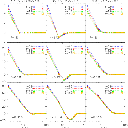
Figure 9: Spatial clustering in the ${\bf D}$ field. We show $\xi_{D}(r)/3=\langle D_{x}D_{x}\rangle=(2\psi_{\perp}+\psi_{\parallel})/3$, $\psi_{\parallel}$ and $\psi_{\perp}$ respectively in left, middle and right panels. The ${\bf D}$ field is spatially clustered at $r\lesssim L_{P}^{-1}$. The mean particle separation $L_{P}=12(f/0.1\%)^{-1/3}{\rm Mpc}/h$ for the specific J1200 simulation.

III.2.3 Spatial correlation in the ${\bf D}$ field

The ${\bf D}$ field is spatially correlated. The spatial correlation can arise from Poisson fluctuation. This is a little bit surprising since Poisson fluctuation is not spatially correlated. The reason is that, for sparse samples, a significant fraction of particles can be assigned to more than one grid point and hence build spatial correlation over scales $\sim L_{P}$. Intrinsic LSS fluctuation creates larger voids, in which spatial correlation over larger separation can be built. More discussion on this issue can be found in paper I.

Following Peebles (1980), we decompose the correlation function into a perpendicular part $\psi_{\perp}$ and a parallel part $\psi_{\parallel}$,

$$\langle D_{i}({\bf x})D_{j}({\bf x}+{\bf r})\rangle_{\bf x}=\psi_{\perp}(r)\delta_{ij}+(\psi_{\parallel}(r)-\psi_{\perp}(r))\hat{r}_{i}\hat{r}_{j}\ .$$ (10)

Here $i,j=x,y,z$ are three Cartesian axes. The averaged correlation function

$$\xi_{\rm D}\equiv\langle{\bf D}({\bf x})\cdot{\bf D}({\bf x}+{\bf r})\rangle_{\bf x}=2\psi_{\perp}(r)+\psi_{\parallel}(r)\ .$$ (11)

Fig. 9 shows the correlation function $\psi_{\perp}$, $\psi_{\parallel}$ and $\xi_{D}/3$, for $f=1\%$, $0.1\%$ and $0.01\%$. As a reminder, the mean simulation particle separation for the J1200 simulation is $L_{P}=12{\rm Mpc}/h(0.1\%/f)^{1/3}$. Indeed, we find non-negligible correlation at $r\lesssim L_{P}$. When $r>L_{P}$, the correlation quickly vanishes and the ${\bf D}$ field can then be treated as a random field of no spatial correlation. This means that to model the sampling artifact at $k\ll 1/L_{P}$, we can treat the ${\bf D}$ field as uncorrelated. However, at $k\gtrsim 1/L_{P}$, the spatial correlation in ${\bf D}$ matters. The leading order approximation for the sampling artifact (Eq. 7) neglects such spatial correlation, so it loses accuracy at $k\gtrsim 1/L_{P}$. Later we will show that the neglected spatial correlation can be implemented to improve the model accuracy.

Similar to the case of $\sigma_{D}$, both the Poisson fluctuation and the intrinsic LSS fluctuation in the particle distribution contribute to $\xi_{D}$. The former does not vary with redshift, while the latter does. Hence we can use the redshift dependence of $\xi_{D}$ to infer the relative importance of the intrinsic LSS fluctuation. For $f\gtrsim 0.1\%$, we observe this redshift dependence. Especially where $\xi_{D}>0$, its strength decreases with increasing redshift. This is caused by decreasing amplitude of the intrinsic LSS fluctuation. The impact of LSS weakens when $f$ ($\bar{n}_{P}$) decreases and hence Poisson fluctuation increases. For $f=1\%$, the impact from intrinsic LSS is very significant. For $f=0.01\%$, the impact is barely visible. For $f=0.1\%$, the impact is neither overwhelming nor negligible.

Hence for $\bar{n}_{P}\gtrsim 6\times 10^{-4}({\rm Mpc}/h)^{-3}$, modelling the spatial correlation in ${\bf D}$ shall take the intrinsic LSS fluctuation into account. This further complicates the modelling of the sampling artifact. For example, a sample of DM particles and a sample of halos with the same number density in the same cosmic volume in general have different sampling artifacts, due to different intrinsic LSS clustering.

III.3 Testing Eq. 7

Our theory, under the approximation of no spatial correlation in ${\bf D}$, predicts through Eq. 7

$$\eta(k|f)\simeq\frac{S(k|f)}{S(k|f=1)}\ .$$ (12)

Since the ${\bf D}$ field is directly measurable in simulations, we can easily evaluate $S(k)\equiv\langle\exp(i{\bf k}\cdot{\bf D})\rangle^{2}$ (Eq. 8) and hence evaluate the above theoretical prediction. In doing so we have automatically included the effect of intrinsic LSS fluctuation in the particle distribution. This differs from the simplified prediction in paper I in which only the Poisson fluctuation is included. We compare Eq. 12 against simulation result in Fig. 3, 4 & 5. We remind that $S(k)$ is evaluated using the exact definition $S(k)\equiv\langle\exp(i{\bf k}\cdot{\bf D})\rangle^{2}$, instead of its Gaussian approximation $\exp(-k^{2}\sigma_{D}^{2}/3)$. Since $S(k)$ does not depend on the direction of $k$, we can choose ${\bf k}=(k,0,0)$. We then have

$$S(k)=\langle\exp(ikD_{x})\rangle^{2}=\exp\left[-y(1-\frac{K_{4}y}{12}+\frac{K_{6}y^{2}}{360}+\cdots)\right]$$

Here, $y\equiv k^{2}\langle D_{x}^{2}\rangle=k^{2}\sigma_{D}^{2}/3$. Fig. 7 & 8 show visible non-Gaussianity in the ${\bf D}$ field ($K_{4,6,\cdots}\neq 0$). Including these non-Gaussian terms in evaulating $S(k)$ is necessary where $y\gtrsim 1$. For this reason, we always use the exact definition to evaluate $S(k)$, instead of using the approximation $S(k)\sim\exp(-y)$.

Eq. 12 shows good to excellent agreement with simulation results. It well reproduces the overall behavior of increasing $1-\eta$ with decreasing $f$ ($\bar{n}_{P}$) and increasing $k$. Furthermore, for $f\gtrsim 1\%$ ($\bar{n}_{P}\gtrsim 6.2\times 10^{-3}({\rm Mpc}/h)^{-3}$), it is accurate to $\sim 1\%$ or better over practically all scales at $k<0.3h/{\rm Mpc}$. For lower number density, the agreement is worse. Nevertheless, it is still reasonably good. For example, the theory predicts $\eta(k=0.1h/{\rm Mpc}|f=0.1\%)=0.82$ at $z=0$, compared to the simulation result $\eta(k=0.1h/{\rm Mpc}|f=0.1\%)=0.87$.

III.4 More accurate ansatz to model the sampling artifact

Agreement at such level is encouraging, however not sufficient if we want to measure the velocity bias of $10^{13}M_{\odot}$ in simulation to $1\%$ level accuracy. These halos have $\bar{n}_{P}\sim 10^{-3}({\rm Mpc}/h)^{-3}$ at $z=0$. The $1\%$ accuracy is required to match the stage IV dark energy surveys such as BigBOSS/MS-DESI Schlegel et al. (2011), Euclid and SKA. To achieve this accuracy, the sampling artifact should be corrected to $1\%$ at least at $k=0.1h/{\rm Mpc}$. Eq. 7 is only able to do so with $\sim 6\%$ accuracy at $k=0.1h/{\rm Mpc}$ for $\bar{n}_{P}=6\times 10^{-4}({\rm Mpc}/h)^{-3}$. So further improvement is needed.

A major source of inaccuracy of Eq. 7 (Eq. 12) is the neglected spatial correlation in ${\bf D}$ when deriving it. Fig. 9 shows that the spatial correlation in ${\bf D}$ is non-negligible when spatial separation is $\lesssim L_{P}$. Hence it must be incorporated appropriately in the modelling. Paper I derives analytical expression for these corrections. It is mathematically solid. Unfortunately it is computationally expensive and is hence hard to implement in numerical evaluation.

Therefore here we propose an approximate but efficient way to incorporate the neglected spatial correlation of ${\bf D}$ into account, with the hope to improve over Eq. 7 (Eq. 12). Using the cumulant expansion theory, Eq. 6 & 8 read

$$S({\bf k},{\bf r})=S(k)e^{k_{i}k_{j}\langle D_{i}D_{j}\rangle+\cdots}\ .$$ (13)

Neglecting all high order terms and approximating $\langle D_{i}D_{j}\rangle$ with the one averaged over all directions, we obtain

$$S({\bf k},{\bf r})\simeq S(k)e^{\frac{1}{3}k^{2}\xi_{D}(r)}\ .$$ (14)

Eq. 4, 5 & 6 suggest that the dominant suppression to $\hat{P}(k)$ comes from $S({\bf k},{\bf r})$ with $r\sim 1/k$. Let us approximate that it comes from a single $r_{\rm eff}=\alpha/k$, where $\alpha\sim 1$ is a unknown constant to be fixed. We then expect

$$\hat{P}_{E}(k) \simeq P_{E}(k)S(k)e^{\frac{1}{3}k^{2}\xi_{D}(r_{\rm eff}=\alpha/k)}$$

$$= P_{E}(k)\langle e^{i{\bf k}\cdot{\bf D}}\rangle^{2}e^{\frac{1}{3}k^{2}\xi_{D}(r_{\rm eff}=\alpha/k)}\ .$$

The derivation is far from strict so we shall only treat the above result as an approximate ansatz. Nevertheless, it is physically motivated, convenient to implement and takes the leading order effect of spatial correlation in ${\bf D}$ into account. (1) It has the correct asymptotic behavior at $k\rightarrow 0$, where the correction vanishes and one recovers the no spatial clustering limit. (2) It has the correct asymptotic behavior at $\alpha\gg 1$. This corresponds to the case of no spatial clustering (Eq. 7). (3) For $k=0.1h/{\rm Mpc}$, correlation at $r=1/k=10{\rm Mpc}/h$ is non-negligible for $f<0.1\%$. Furthermore, $\xi_{D}>0$ there. So the above formula predicts larger $\eta$ and hence better agreement with simulation result.

We do not attempt to find the best-fit $\alpha$. Instead, we demonstrate the improvement over Eq. 7 with $\alpha=1/2$ in Fig. 3, 4 & 5. The improvement is significant. For example, it improves the theory accuracy of $\eta(k|f=0.1\%)$ at $k=0.1h/{\rm Mpc}$ from $\sim 6\%$ to $1\%$. The improvement for $f=0.01\%$ is even more significant.

IV Self-calibration and discussion

The ultimate goal of the current paper and paper I is to correct for the sampling artifact robustly in order to measure the volume weighted halo velocity power spectrum and halo velocity bias accurately. The sampling artifact is completely determined by $\bar{n}_{P}$ and the intrinsic LSS fluctuation. Based on general argument on the two factors, we obtain a quick-to-implement ansatz (Eq. III.4) on how the sampling artifact suppresses the measured velocity power spectrum.

We have demonstrated that it works for a variety of DM samples with the mean particle number density over 4 decades ($6\times 10^{-1}({\rm Mpc}/h)^{-3}$-$6\times 10^{-5}({\rm Mpc}/h)^{-3}$), and typical intrinsic LSS clustering from $z=2$ to $z=0$. The derivation on Eq. III.4 is general in the sense that it assumes no special form of intrinsic LSS fluctuation. Hence as long as it works for DM particles, it should work equally well for DM halos. With this reasonable extrapolation, we believe the following self-calibration works for DM halos,

$$\hat{P}_{E}(k)\rightarrow\frac{\hat{P}_{E}(k)}{\langle e^{i{\bf k}\cdot{\bf D}}\rangle^{2}e^{\frac{1}{3}k^{2}\xi_{D}(r_{\rm eff}=\alpha/k)}}.$$ (16)

We caution that now the ${\bf D}$ field is that of DM halos, which differs from that of DM particles. This measure of the velocity power spectrum at $k\leq 0.1h/{\rm Mpc}$ should be essentially free of the sampling artifact, at the level of $1\%$ for $10^{13}M_{\odot}$ halos or less massive ones at $z=0$. This will then allow us to measure the real halo velocity bias, free of otherwise severe systematic error from the sampling artifact. We will present such measurements in Zheng et al. (2014), which belongs to our ongoing efforts to understand the velocity field, redshift shift space distortion and velocity reconstruction in spectroscopic redshift surveys Zhang et al. (2013); Zheng et al. (2013).

The current paper focuses on the sampling artifact in the gradient part of the velocity field. The curl part of the velocity also suffers from numerical artifacts such as the alias effect Pueblas and Scoccimarro (2009) and the sampling artifact Zhang et al. (2015); Zheng et al. (2013). We can use the same method (Eq. 1) to quantify the sampling artifact in the curl part of the velocity field. One subtlety is that numerical artifacts in the curl velocity are much more severe, so higher simulation resolution is required than the J1200 that we have analyzed. This topic will be explored elsewhere.

V Acknowledgement

This work was supported by the National Science Foundation of China (Grants No. 11025316, No. 11121062, No. 11033006, No. 11320101002, and No. 11433001), National Basic Research Program of China (973 Program 2015CB857000), the NAOC-Templeton Beyond the Horizon program, the CAS Strategic Priority Research Program ”The Emergence of Cosmological Structures” of the Chinese Academy of Sciences, Grant No. XDB09000000 and the key laboratory grant from the Office of Science and Technology, Shanghai Municipal Government (No. 11DZ2260700). P. J. Z. gratefully acknowledges the support of the National Science Foundation through Grant No. PHYS-1066293 and thanks the Simons Foundation and, for their hospitality, the Aspen Center for Physics, where part of the work was done. Y. Z. thanks Yu Yu, Yanchuan Cai, and Jiawei Shao for the useful discussions.

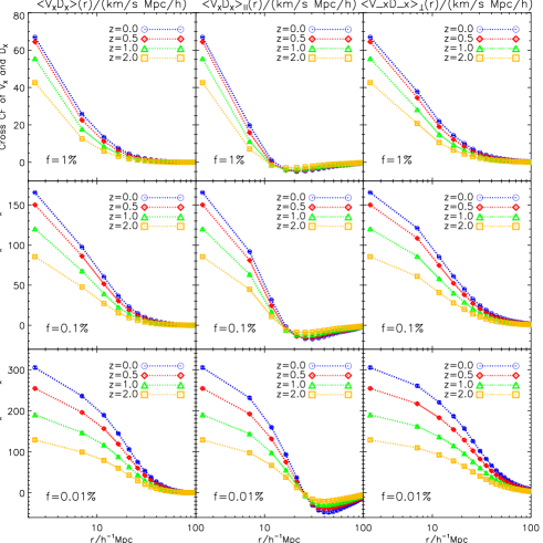
Figure 10: The ${\bf v}$-${\bf D}$ correlation detected in simulations. The left, middle and right panels are $\langle v_{x}D_{x}\rangle=(2\langle vD\rangle_{\perp}+\langle vD\rangle_{\parallel})/3$, $\langle vD\rangle_{\parallel}$ and $\langle vD\rangle_{\perp}$ respectively. The ${\bf v}$-${\bf D}$ correlation is weak in that $\langle vD\rangle\ll\sigma_{v}\sigma_{D}$. However, it is in principle a significant aspect of the sampling artifact and should be taken into account, especially at $k>0.1h/{\rm Mpc}$ for sparse samples.

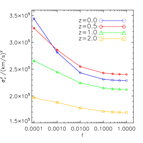
Figure 11: $\sigma_{v}^{2}\equiv\langle\hat{v}^{2}\rangle$ as a function of $\bar{n}_{P}=0.62f({\rm Mpc}/h)^{-3}$ and $z$. Its variation with $f$ is caused by correlation between the velocity (signal) field and the ${\bf D}$ (sampling) field (the appendix). It highlights another aspect of the sampling artifact. In contrast to underestimation of the velocity power spectrum at large scale, the sampling artifact overestimates the velocity dispersion. It is likely responsible for the overestimation of the velocity power spectrum at small scales and low $f$, observed in Fig. 5 for the case of $f=0.01\%$.

Appendix A More aspects of the sampling artifact

The $\eta$ measurement for $f=0.01\%$ (Fig. 5) shows abnormal behaviors at $k\gtrsim 0.08h/{\rm Mpc}$. The most significant is the turn-over at $k\sim 0.08h/{\rm Mpc}$ and the eventual $\eta>1$ at $k\gtrsim 0.15h/{\rm Mpc}$, for $z=0$. Another anomaly is that $\eta$ decreases with increasing redshift, in contrast to our theoretical expectation and the cases of $f\gtrsim 0.1\%$. The two anomalies are likely related. These anomalies are not statistical flukes, since we have run many more realizations of DM sub-samples and found the same anomalies. They may imply either unknown numerical artifacts or inappropriate understanding of the sampling artifact in very sparse samples.

Unfortunately so far we do not have any real insight to solve these issues. We are only able to discuss/evaluate some possibilities, and we caution the readers that this list is likely not exhaustive.

• Transport of power of ${\bf v}$ across scales by the field ${\bf D}$. This is caused by spatial correlation of the ${\bf D}$ field, exactly analogous to the deflection field in CMB lensing Seljak (1996). Where the real signal is weak, we may find overestimation of the velocity power spectrum. This point can be demonstrated by a toy model, in which $P_{ij}({\bf k})=A_{ij}$ if ${\bf k}={\bf k}_{*}$ and zero otherwise. $\hat{P}_{ij}({\bf k}_{*})=A_{ij}W({\bf k}_{*},{\bf 0})=A_{ij}S(k_{*})<A_{ij}=P({\bf k}_{*})$. The lost power is transported to other modes, $\hat{P}_{ij}({\bf k}\neq{\bf k}_{*})=A_{ij}W({\bf k}_{*},{\bf k}_{*}-{\bf k})\neq 0$. Is it sufficient to explain the observed anomalies in Fig. 5? We notice that the clustering strength of the ${\bf D}$ field changes little between $z=0$ and $z=2$ (Fig. 9), while $\eta$ increases dramatically at $k=0.1h/{\rm Mpc}$ from $z=2$ to $z=0$. This implies that, the transport of power of ${\bf v}$ by the ${\bf D}$ field is not the major cause of the observed anomalies in Fig. 5.

• A more likely cause is the ${\bf v}$-${\bf D}$ correlation, neglected in the theoretical modelling. It is distinctively different to CMB lensing, in which the lensing field and primary CMB have no cross-correlation. As discussed in paper I, the ${\bf D}$ field is spatially correlated to the velocity field. It can not only transport power across scales, but also generate extra power in ${\bf v}$. This correlation is neglected in Eq. 4 and all results derived based on Eq. 4 (refer to more details in paper I).

Appendix B The detected ${\bf v}$-${\bf D}$ correlation and its impact on the sampling artifact

The ${\bf v}$-${\bf D}$ correlation is inevitable since the intrinsic LSS fluctuation, a source of ${\bf D}$, correlates with ${\bf v}$. We confirm its existence by simulations (Fig. 10). Like the case of auto correlation in ${\bf D}$, the cross correlation can also be decomposed into two coordinate independent components,

$$\langle v_{i}({\bf x})D_{j}({\bf x}+{\bf r})\rangle=\langle vD\rangle_{\perp}\delta_{ij}+(\langle vD\rangle_{\parallel}-\langle vD\rangle_{\perp})\hat{r}_{i}\hat{r}_{j}\ .$$ (17)

The measured cross correlation is weak, comparing to the auto power. For example, for $f=0.1\%$, $\sigma_{D}\sigma_{v}\simeq 2400$ km/$s$ Mpc$/h$. So $\langle vD\rangle\ll\sigma_{v}\sigma_{D}/3$. This is expected, since only the part of ${\bf D}$ sourced by the intrinsic LSS fluctuation is correlated with ${\bf v}$.

We have neglected this complexity of ${\bf v}$-${\bf D}$ correlation in modelling the sampling artifact. This is a major drawback of our theoretical modelling. In particular, it could be the major course of the observed anomalies in Fig. 5 at $k\gtrsim 0.1h/{\rm Mpc}$. It may also be partly responsible for the discrepancy between the simplified theoretical modelling and simulation results in Fig. 4. Unfortunately, we are not able to implement it into quantitative theoretical calculation yet. Therefore we are not able to directly testify the above speculations. Nevertheless, we can prove that it indeed has significant impact on a highly related statistics, $\langle\hat{v}^{2}\rangle$.

If this correlation is indeed negligible, we prove in §C a unbiased velocity dispersion measurement, $\langle\hat{v}^{2}\rangle=\langle v^{2}\rangle$. Hence $\langle\hat{v}^{2}\rangle$ should be independent of the particle fraction $f$. However, simulations show that $\langle\hat{v}^{2}\rangle$ increases with decreasing $f$ (Fig. 11). It clearly proves the significance of correlation between ${\bf v}$ and ${\bf D}$. It causes the velocity dispersion to be overestimated. For $f=0.01\%$, the overestimation reaches $\sim 20\%$ at $z=2$ and $\sim 50\%$ at $z=0$. Since $\langle v^{2}\rangle$ is the integral of the power spectrum, overestimation in $\langle v^{2}\rangle$ must also show up as overestimation of the power spectrum at certain scales. Hence it should be responsible for the observed anomalies in Fig. 5.

This overestimation of $\langle v^{2}\rangle$ is a new impact of the sampling artifact. It arises from the fact that the weighting assigned to each particle is correlated with the velocity (signal) field. On the average, the weighting of each particle in the volume weighted scheme is $\propto(1+\delta)^{-1}$. $\delta$ is the combination of the underlying DM density fluctuation and Poisson fluctuation. The Poisson fluctuation is uncorrelated with the velocity field. However, the intrinsic fluctuation is positively correlated with the local velocity dispersion, resulting in a positive correlation between $\delta$ and the local velocity dispersion. The weighting $\propto(1+\delta)^{-1}$ then suppresses contribution of high density/high velocity dispersion regions. Sparser samples have larger Poisson fluctuation and hence weaker correlation between the simulated $\delta$ and the local velocity dispersion. Therefore it suffers from weaker suppression of high real density/high velocity dispersion regions. So decreasing the particle number density increases $\langle\hat{v}^{2}\rangle$.

The same intrinsic LSS fluctuation causing correlation between the weghting and the velocity signal also causes ${\bf v}$-${\bf D}$ correlation. So the two explanations are consistent.

Appendix C $\langle\hat{v}^{2}\rangle=\langle v^{2}\rangle$ if ${\bf v}$ and ${\bf D}$ are uncorrelated

For brevity, we work at the limit of infinite box size and infinitesimal grid size. The proof for finite box size and non-zero grid size is similar.

$$\langle\hat{v}^{2}\rangle = \int\hat{v}^{2}({\bf x})\frac{d^{3}{\bf x}}{V}$$

$$= \int\langle{\bf v}({\bf k})\cdot{\bf v}({\bf q})e^{i({\bf k}+{\bf q})\cdot{\bf D}}\rangle e^{i({\bf k}+{\bf q})\cdot{\bf x}}\frac{d^{3}{\bf k}d^{3}{\bf q}d^{3}{\bf x}}{(2\pi)^{6}V}\ .$$

Here $V=\int d^{3}{\bf x}$ is the total volume. When ${\bf v}$ and ${\bf D}$ are uncorrelated,

$$\langle{\bf v}({\bf k})\cdot{\bf v}({\bf q})e^{i({\bf k}+{\bf q})\cdot{\bf D}}\rangle\rightarrow\langle{\bf v}({\bf k})\cdot{\bf v}({\bf q})\rangle\langle e^{i({\bf k}+{\bf q})\cdot{\bf D}}\rangle$$

$$=P_{v}(k)(2\pi)^{3}\delta_{3D}({\bf k}+{\bf q})\langle e^{i({\bf k}+{\bf q})\cdot{\bf D}}\rangle$$

$$=P_{v}(k)(2\pi)^{3}\delta_{3D}({\bf k}+{\bf q})\ .$$

We then finally prove

$$\langle\hat{v}^{2}\rangle=\int P_{v}(k)\frac{d^{3}{\bf k}}{(2\pi)^{3}}\frac{d^{3}{\bf x}}{V}=\langle v^{2}\rangle\ .$$ (19)

This means that, if the signal (${\bf v}$) and the sampling field ${\bf D}$ are uncorrelated, the estimation of velocity dispersion will be unbiased. A corollary is that, the measured $\langle\hat{v}^{2}\rangle$ should not depend on the particle fraction $f$, if ${\bf v}$ and ${\bf D}$ are uncorrelated. Then if $\langle\hat{v}^{2}\rangle$ depends on $f$ ($\bar{n}_{P}$), there must be non-negligible correlation between ${\bf v}$ and ${\bf D}$. The observed significant dependence of $\langle\hat{v}^{2}\rangle$ on the particle number density (Fig. 11) then provides an indirect, nevertheless solid, evidence of ${\bf v}$-${\bf D}$ correlation. This is further supported by the direct measurement in Fig. 10.

References

- Zhang et al. (2015) P. Zhang, Y. Zheng, and Y. Jing, Phys. Rev. D 91, 043522 (2015), eprint 1405.7125.
- Bernardeau and van de Weygaert (1996) F. Bernardeau and R. van de Weygaert, MNRAS 279, 693 (1996).
- Watkins and Feldman (2014) R. Watkins and H. A. Feldman, ArXiv e-prints (2014), eprint 1407.6940.
- Johnson et al. (2014) A. Johnson, C. Blake, J. Koda, Y.-Z. Ma, M. Colless, M. Crocce, T. M. Davis, H. Jones, J. R. Lucey, C. Magoulas, et al., ArXiv e-prints (2014), eprint 1404.3799.
- Zheng et al. (2014) Y. Zheng, P. Zhang, and Y. Jing, ArXiv e-prints (2014), eprint 1410.1256.
- Schlegel et al. (2011) D. Schlegel, F. Abdalla, T. Abraham, C. Ahn, C. Allende Prieto, J. Annis, E. Aubourg, M. Azzaro, S. B. C. Baltay, C. Baugh, et al., ArXiv e-prints (2011), eprint 1106.1706.
- Bardeen et al. (1986) J. M. Bardeen, J. R. Bond, N. Kaiser, and A. S. Szalay, Astrophys. J. 304, 15 (1986).
- Desjacques (2008) V. Desjacques, Phys. Rev. D 78, 103503 (2008), eprint 0806.0007.
- Desjacques and Sheth (2010) V. Desjacques and R. K. Sheth, Phys. Rev. D 81, 023526 (2010), eprint 0909.4544.
- Zheng et al. (2013) Y. Zheng, P. Zhang, Y. Jing, W. Lin, and J. Pan, Phys. Rev. D 88, 103510 (2013), eprint 1308.0886.
- Jennings et al. (2014) E. Jennings, C. M. Baugh, and D. Hatt, ArXiv e-prints (2014), eprint 1407.7296.
- Jing et al. (2007) Y. P. Jing, Y. Suto, and H. J. Mo, Astrophys. J. 657, 664 (2007), eprint arXiv:astro-ph/0610099.
- Jing (2005) Y. P. Jing, Astrophys. J. 620, 559 (2005), eprint arXiv:astro-ph/0409240.
- Pueblas and Scoccimarro (2009) S. Pueblas and R. Scoccimarro, Phys. Rev. D 80, 043504 (2009), eprint 0809.4606.
- Koda et al. (2013) J. Koda, C. Blake, T. Davis, M. Scrimgeour, G. B. Poole, and L. S. Smith, ArXiv e-prints (2013), eprint in preparation.
- Peebles (1980) P. J. E. Peebles, The large-scale structure of the universe (1980).
- Zhang et al. (2013) P. Zhang, J. Pan, and Y. Zheng, Phys. Rev. D 87, 063526 (2013), eprint 1207.2722.
- Seljak (1996) U. Seljak, Astrophys. J. 463, 1 (1996), eprint astro-ph/9505109.