Pairwise thermal entanglement in Ising-XYZ diamond chain structure in an external magnetic field

Abstract

Quantum entanglement is one of the most fascinating types of correlation that can be shared only among quantum systems. The Heisenberg chain is one of the simplest quantum chains which exhibits a reach entanglement feature, due to the Heisenberg interaction is quantum coupling in the spin system. The two particles were coupled trough XYZ coupling or simply called as two-qubit XYZ spin, which are the responsible for the emergence of thermal entanglement. These two-qubit operators are bonded to two nodal Ising spins, and this process is repeated infinitely resulting in a diamond chain structure. We will discuss two-qubit thermal entanglement effect on Ising-XYZ diamond chain structure. The concurrence could be obtained straightforwardly in terms of two-qubit density operator elements, using this result, we study the thermal entanglement, as well as the threshold temperature where entangled state vanishes. The present model displays a quite unusual concurrence behavior, such as, the boundary of two entangled regions becomes a disentangled region, this is intrinsically related to the XY-anisotropy in the Heisenberg coupling. Despite a similar property had been found for only two-qubit, here we show in the case of a diamond chain structure, which reasonably represents real materials.

I Introduction

In the last decade, many efforts were dedicated to characterizing qualitatively and quantitatively the entanglement properties of condensed matter systems which are the natural candidate to apply for quantum communication, as well as quantum information. In this sense, it is quite interesting to study the entanglement of solid state systems such as spin chainsqubit-Heisnb . The Heisenberg chain is one of the simplest quantum chains which exhibit a reach entanglement feature, due to the Heisenberg interaction is a nonlocal correlation between quantum systemskamta .

Quantum entanglement, with its applications to quantum phase transitions of strongly correlated spin systems and its experimental implementation in optical lattices, was considered, in particular, for one-dimensional systems. Diverging entanglement length without quantum phase transition was found in a localizable entanglement (LE) for valence bond solids (VBSs), since the correlation length remains finitevestraete . This aforementioned is a rather new and remarkable result regarding the entanglement properties of VBS quantum spin ground states. A theory for localizable entanglement was developed based on matrix product states from the density matrix renormalization group (DMRG) method and applied to VBS statespopp . In reference garcia , an experimental implementation was proposed for VBSs of the spin-1 Heisenberg Hamiltonians and ladders, and a method was proposed directly to measure quantum observables that are not accessible in standard materials in condensed matter.

Motivated by real materials such as $\mathrm{Cu_{3}(CO_{3})_{2}(OH)_{2}}$ known as azurite, which is an interesting quantum antiferromagnetic model described by Heisenberg model on generalized diamond chain. Honecker et al. honecker studied the dynamic and thermodynamic properties for this model. Moreover, the thermodynamics of the Ising-Heisenberg model on diamond-like chain was also widely discussed in referencescanova06 ; vadim ; valverde ; lisnii-11 . The motivation to research the Ising-XYZ diamond chain model is based in some recent works. According to the experiments of the natural mineral azurite, theoretical calculations of Ising-XXZ model, as well as the experimental result of the exchange dimer (interstitial sites) parameter and their descriptions of the various theoretical models. The 1/3 magnetization plateau, the double peaks both in the magnetic susceptibility and specific heat, was observed in the experimental measurementsrule ; kikuchi . It should be noted that the dimer (interstitial sites) are exchange much more strong than those nodal sites. Since dimmer interaction is much higher than the rest, it can be represented as an exactly solvable Ising-Heisenberg model. In addition, experimental data on the magnetization plateau coincides approximately with Ising-Heisenberg modelcanova06 ; ananikian ; chakh .

Recently several investigation are focusing on thermal entanglement with Heisenberg coupling qubits as well as assuming some finite chain structure. The thermal entanglement of isotropic Heisenberg spin chain has been studied in the absence wang and the presence of an external magnetic field X-Wang ; arnesen . The entanglement of the two-qubit isotropic Heisenberg system decreases when the temperature increases which vanishes beyond a threshold temperature $T_{th}$. However, two qubits with XYZ coupling displays quite interesting thermal entanglement behaviorG. Rigolin , such as more than one threshold temperature. On the other hand, an unusual property of entanglement also was considered in an alternating Ising and Heisenberg spins in simple one-dimensional chainm-rojas14 , where despite at zero temperature there is no any evidence of entanglement, then rise a small amount of concurrence indicating the system has a thermal entanglement between two Heisenberg spins. More over this result was confirmed by theoretical model lazaryan by Gibbs-Bogoliubov approach (Heisenberg-Ising model) with experimental results of natural material azurite kikuchi .

This paper is organized as follow: in Sec. II we present the Ising-XYZ model on diamond chain and its phase diagram at zero temperature. Further, in Sec. III, we present the exact thermodynamic solution of the model. In Sec. IV, we have discussed the thermal entanglement of Heisenberg reduced density operator of the model, such as concurrence and threshold temperature. Finally, Sec. V contains the concluding remarks.

II The Ising-XYZ chain on diamond chain structure

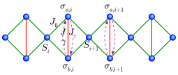
Figure 1: (Color Online) Schematic representation of Ising-XYZ chain on diamond structure, $\sigma_{a,i}$ and $\sigma_{i,b}$ are Heisenberg spins, while $S_{i}$ corresponds to Ising spins.

The thermal entanglement of Ising-Heisenberg diamond chain already was discussed. Here we extend this model in agreement with the motivation discussed above. Therefore, let us consider an Ising-XYZ diamond chain structure as illustrated schematically in figure 1. Thus, the Ising-XYZ Hamiltonian becomes

$$H= -\sum_{i=1}^{N}\left[J(1+\gamma)\sigma_{a,i}^{x}\sigma_{b,i}^{x}+J(1-\gamma)\sigma_{a,i}^{y}\sigma_{b,i}^{y}+\right.$$

$$+J_{z}\sigma_{a,i}^{z}\sigma_{b,i}^{z}+J_{0}(\sigma_{a,i}^{z}+\sigma_{b,i}^{z})(S_{i}+S_{i+1})+$$

$$\left.+h(\sigma_{a,i}^{z}+\sigma_{b,i}^{z})+\frac{h}{2}(S_{i}+S_{i+1})\right],$$ (1)

where $\sigma_{a(b)}^{\alpha}$ are the Pauli matrix with $\alpha=\{x,y,z\}$, and $S$ corresponds to the Ising spins, whereas $\gamma$ is the XY-anisotropy parameter.

After diagonalizing the XYZ term, we have the following eigenvalues for XYZ dimer in terms of nodal spin chain $\mu=S_{i}+S_{i+1}$,

$$\varepsilon_{1,4}= -h\frac{\mu}{2}-\frac{J_{z}}{4}\pm\Delta(\mu),$$ (2)

$$\varepsilon_{2,3}= -h\frac{\mu}{2}\mp\frac{J}{2}+\frac{J_{z}}{4},$$ (3)

wherein

$$\Delta(\mu)=\sqrt{\left(h+J_{0}\mu\right)^{2}+\tfrac{1}{4}J^{2}\gamma^{2}},$$ (4)

with the corresponding eigenvectors in terms of standard basis $\{|\begin{smallmatrix}-\\ -\end{smallmatrix}\rangle,|\begin{smallmatrix}-\\ +\end{smallmatrix}\rangle,|\begin{smallmatrix}+\\ -\end{smallmatrix}\rangle,|\begin{smallmatrix}+\\ +\end{smallmatrix}\rangle\}$ are given respectively by

$$|\varphi_{1,4}\rangle =N_{\pm}\left(\alpha_{\pm}|\begin{smallmatrix}+\\ +\end{smallmatrix}\rangle+|\begin{smallmatrix}-\\ -\end{smallmatrix}\rangle\right),$$ (5)

$$|\varphi_{2,3}\rangle =\tfrac{1}{\sqrt{2}}\left(|\begin{smallmatrix}-\\ +\end{smallmatrix}\rangle\pm|\begin{smallmatrix}+\\ -\end{smallmatrix}\rangle\right),$$ (6)

where $\alpha_{\pm}=\frac{-J\gamma}{2h+2J_{0}\mu\pm 2\Delta(\mu)}$, and $N_{\pm}=\frac{1}{\sqrt{1+\alpha_{\pm}^{2}}}$.

It is important to recall that the pairwise entanglement between Heisenberg spins at zero temperature is entangled for any Hamiltonian parameters, unless for the limiting case becomes disentangled region. Which will be illustrated in the zero temperature limit of the phase transition.

This model is somewhat opposite to that proposed in reference m-rojas14 , where at zero temperature there was no thermal entanglement.

II.1 Phase diagram of Ising-XYZ on diamond chain

Here, we start our discussion regarding to the phase diagram at zero temperature, first we assume the chain is in the absence of magnetic field. Thus, we illustrate the phase diagram in figure 2(a), as a function of $J_{0}/J$ against $\gamma$ assuming a fixed value $J_{z}/J=0$ and $h/J=0$. Where, we show two phases one Ising spin ferromagnetic with Heisenberg spin modulated ferromagnetic simply denoted by modulated ferromagnetic ($FMF$) phase, and the Ising spin frustrated region ($IFR$).

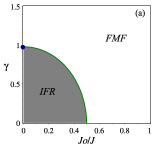
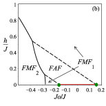
Figure 2: Zero temperature phase diagram for the limiting case Ising-XY ($J_{z}/J=0$ ) and in absence of magnetic field. (a) Phase diagram $J_{0}/J$ against $\gamma$, for a fixed value $h/J=0$. (b) For $J_{0}/J$ versus $h/J$ and assuming $\gamma=0.95$.

The explicit representations of $FMF$ states are expressed below

$$|FMF_{1}\rangle= \overset{N}{\underset{i=1}{\prod}}|\varphi_{4}\rangle_{i}\otimes|+\rangle_{i},$$ (7)

$$|FMF_{2}\rangle= \overset{N}{\underset{i=1}{\prod}}|\varphi_{4}\rangle_{i}\otimes|-\rangle_{i},$$ (8)

and the ground state energy are given by

$$E_{FMF_{1}}= -\frac{h}{2}-\sqrt{\left(h+J_{0}\right)^{2}+\tfrac{1}{4}J^{2}\gamma^{2}},$$ (9)

$$E_{FMF_{2}}= \frac{h}{2}-\sqrt{\left(h-J_{0}\right)^{2}+\tfrac{1}{4}J^{2}\gamma^{2}},$$ (10)

it is worth to notice that $FMF_{1}$ and $FMF_{2}$ are degenerated at null magnetic field, what we denote simply by $FMF$ region. At first glance the states $FMF_{1}$ and $FMF_{2}$ seem equivalents under total spin inversion; however, the state $|\varphi_{4}\rangle$ under spin inversion leads to a different state. Therefore, the states $FMF_{1}$ and $FMF_{2}$ are no longer equivalents.

Nevertheless, with no magnetic field, the model illustrates a frustrated region, which is represented as

$$|IFR\rangle=\overset{N}{\underset{i=1}{\prod}}|\varphi_{2}\rangle_{i}\otimes|S\rangle_{i},$$ (11)

with ground state energy given by $E_{IFR}=-\frac{|J|}{2}.$

Observe, that $IFR$ phase has a residual entropy $\mathcal{S}_{0}=\kappa_{B}\ln(2)$, the term 2 becomes from two possible orientation of $S$ in eq.(11). The green curve contouring the IFR region given by $\gamma=\sqrt{1-4J_{0}^{2}}$ has a residual entropy $\mathcal{S}_{0}=\kappa_{B}\ln(3)$, while the blue point corresponds to a residual entropy $\mathcal{S}_{0}=\kappa_{B}\ln(4)$.

A similar phase diagram at zero temperature is displayed in figure 2(b) as a function of $J_{0}/J$ and $h/J$ for a fixed value $\gamma=0.95$ and $J_{z}/J=0$, the thick red line has a residual entropy $\mathcal{S}_{0}=\kappa_{B}\ln(2)$, and the green (gray) circle corresponds to a frustrated point with residual entropy given by $\mathcal{S}_{0}=\kappa_{B}\ln(3)$, while the dashed line curve given by $h/J=\pm\frac{\sqrt{39}}{40}-\frac{J_{0}}{J}$ (upper lower respectively) has a residual entropy $\mathcal{S}_{0}=\kappa_{B}\ln(2)$.

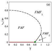
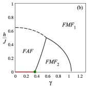
Figure 3: Phase diagram at zero temperature for the Ising-$XY$ diamond chain in units of $J$, for $\gamma$ versus $h/J$, assuming $J_{0}/J=-0.3$. (a) $J_{z}/J=0$. b) $J_{z}/J=0.3$.

In figure 3(a) is displayed the phase diagram at zero temperature $\gamma$ against $h/J$ for a fixed value $J_{0}/J=-0.3$ and $J_{z}/J=0$, the thick red line corresponds to Ising frustrated ($IFR$) region in a zero magnetic field, while the dashed line corresponds to a non-zero Heisenberg frustrated ($HFR$) phase. Furthermore, is displayed three phase: one $FAF$ phase,$FMF_{1}$, and another $FMF_{2}$ phase, given by states (7) and (8). Similarly, phase diagram at zero temperature is displayed in figure 3(b) as a function of $\gamma$ and $h/J$ for fixed value $J_{0}/J=-0.3$ and $J_{z}/J=0.3$, the thick red line and dashed line and the green (gray) circle have the same meaning as for the case (a).

An explicit representation of $FAF$ state is expressed below

$$|FAF\rangle= \overset{N}{\underset{i=1}{\prod}}|\varphi_{2}\rangle_{i}\otimes|+\rangle_{i},$$ (12)

and its ground state energy is given by $E_{FAF}=-\frac{J+h}{2}.$

Particularly, when $\gamma=\sqrt{1-4(J_{0}+h)^{2}}$, we obtain frustration state with magnetic field, given by the state

$$|HFR\rangle=\overset{N}{\underset{i=1}{\prod}}|\varphi_{2(4)}\rangle_{i}\otimes|+\rangle_{i},$$ (13)

with its corresponding ground state energy given by $E_{HFR}=-\frac{|J|+h}{2}.$

It is worth to mention that $HFR$ phase (dashed line in figures 2 and 3) has also a residual entropy $\mathcal{S}_{0}=\kappa_{B}\ln(2)$. At low temperatures residual entropies have common features with thermal entanglement. Comparing the fig. 3(b) and the fig. 4(a) in next section one can observe that fact.

One can also easily verify the $ab$-dimer are entangled in all region illustrated in the phase diagram, only limiting cases could lead to disentangled regions such as the discussed in Ising-XXZ chainspra .

III Thermodynamics

The Ising-XYZ diamond chain can be solved exactly using the decoration transformationSyozi ; Fisher ; phys-A-09 ; strecka pla together with the usual transfer matrix technique baxter-book . So, let us start considering the partition function as follow

$$\mathbb{\mathcal{Z}}={\rm tr}\left({\rm e}^{-\beta H}\right),$$ (14)

where $\beta=1/\kappa_{B}T$, with $\kappa_{B}$ being the Boltzmann constant and $T$ is the absolute temperature, and the Hamiltonian $H$ is given by eq.(1). The transfer matrix of the model can be expressed by

$$T=\left[\begin{array}[]{cc}w(2)&w(0)\\ w(0)&w(-2)\end{array}\right],$$ (15)

where the Boltzmann factors is expressed by

$$w(\mu)=2{\rm e}^{\frac{\beta\mu h}{2}}\left[{\rm e}^{-\frac{\beta J_{z}}{4}}\cosh\left(\tfrac{\beta J}{2}\right)+{\rm e}^{\frac{\beta J_{z}}{4}}\cosh\left(\beta\Delta(\mu)\right)\right],$$ (16)

and transfer matrix eigenvalues, become

$$\lambda_{\pm}=w(2)+w(-2)\pm\sqrt{\left(w(2)-w(-2)\right)^{2}+4w(0)^{2}}.$$ (17)

To study the thermodynamic properties we will use the exact free energy per unit cell in thermodynamic limit

$$f=-\frac{1}{\beta}\underset{N\rightarrow+\infty}{\lim}\frac{\ln\mathcal{Z}}{N}=-\frac{1}{\beta}\ln\lambda_{+}.$$

Next, let us calculate the thermal entanglement behavior between $ab$-dimer of our model investigated.

IV Pairwise Thermal Entanglement

Now let us start our discussion regarding the quantum entanglement of the Ising-XYZ diamond chain, recalling that a two-qubits with XYZ coupling was discussed in reference G. Rigolin . As a measure of entanglement for two arbitrary mixed states of dimers, we use the quantity called concurrencewootters , which is defined in terms of reduced density matrix $\rho$ of two mixed states

$$\mathcal{C}(\rho)=\max\{{0,2\Lambda_{{\rm max}}-\text{{tr}}\sqrt{R}}\},$$ (18)

assuming $R=\rho\sigma^{y}\otimes\sigma^{y}\rho^{*}\sigma^{y}\otimes\sigma^{y},$ where $\Lambda_{{\rm max}}$ is the largest eigenvalue of the matrix $\sqrt{R}$ and $\rho^{*}$ represent the complex conjugate of matrix $\rho$, with $\sigma^{y}$ being the Pauli matrix.

Consequently the concurrence between $ab$-dimer becomes

$$\mathcal{C}=\max\{0,|\rho_{14}|-{\rho_{22}\rho_{33}},|\rho_{23}|-\sqrt{\rho_{11}\rho_{44}}\},$$ (19)

where the $\rho_{ij}$ are the elements of the density matrix. For the case of an infinite chain, the reduced density operator elementsbukman could be expressed in terms of the correlation function between two entangled particlesamico ,

$$\rho_{11}= \tfrac{1}{4}+\langle\sigma_{a}^{z}\sigma_{b}^{z}\rangle+\langle\sigma_{a}^{z}\rangle,$$ (20)

$$\rho_{22}=\rho_{33}= \tfrac{1}{4}-\langle\sigma_{a}^{z}\sigma_{b}^{z}\rangle,$$ (21)

$$\rho_{44}= \tfrac{1}{4}+\langle\sigma_{a}^{z}\sigma_{b}^{z}\rangle-\langle\sigma_{a}^{z}\rangle,$$ (22)

$$\rho_{14}= \langle\sigma_{a}^{x}\sigma_{b}^{x}\rangle-\langle\sigma_{a}^{y}\sigma_{b}^{y}\rangle,$$ (23)

$$\rho_{23}= \langle\sigma_{a}^{x}\sigma_{b}^{x}\rangle+\langle\sigma_{a}^{y}\sigma_{b}^{y}\rangle.$$ (24)

It is worth to mention that the zero temperature entanglement for $ab$-dimer is maximally entangled in $FAF$ region $\mathcal{C}=1$, while in the region $FMF$ the concurrence depends on Hamiltonian parameters, which is given by $\mathcal{C}=\frac{|J\gamma|}{2\sqrt{\left(J_{0}+h\right)^{2}+\frac{1}{4}J^{2}\gamma^{2}}}.$

However, at finite temperature, each expected values become temperature dependent quantities which are expressed as

$$\langle\sigma_{a}^{x}\sigma_{b}^{x}\rangle= {\rm e}^{\beta\frac{h}{2}}\tfrac{\tfrac{\Delta(1)}{2}{\rm e}^{-\beta\frac{2h+J_{z}}{4}}\sinh(\tfrac{\beta J}{2})+\tfrac{J\gamma}{4}{\rm e}^{\beta\frac{J_{z}}{4}}\sinh(\beta\Delta(1))}{\Delta(1)\lambda_{+}},$$ (25)

$$\langle\sigma_{a}^{y}\sigma_{b}^{y}\rangle= {\rm e}^{\beta\frac{h}{2}}\tfrac{\tfrac{\Delta(1)}{2}{\rm e}^{-\beta\frac{J_{z}}{4}}\sinh(\tfrac{\beta J}{2})-\tfrac{J\gamma}{4}{\rm e}^{\beta\frac{J_{z}}{4}}\sinh(\beta\Delta(1))}{\Delta(1)\lambda_{+}},$$ (26)

$$\langle\sigma_{a}^{z}\sigma_{b}^{z}\rangle= {\rm e}^{\beta\frac{h}{2}}\tfrac{{\rm e}^{\beta\frac{J_{z}}{4}}\cosh(\tfrac{\beta J}{2})-{\rm e}^{-\beta\frac{J_{z}}{4}}\cosh(\beta\Delta(1))}{2\lambda_{+}},$$ (27)

$$\langle\sigma_{a}^{z}\rangle= {\rm e}^{\beta\frac{2h+J_{z}}{4}}\sinh(\beta\Delta(1))\frac{J_{0}+h}{\Delta(1)\lambda_{+}},$$ (28)

Alternatively, we can obtain also equivalent result using the approach described in reference spra .

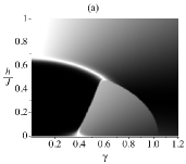
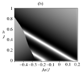
Figure 4: Density-plot thermal entanglement in the low temperature limit $T/J=0.01$. (a) Concurrence as a function of $\gamma$ against $h/J$ assuming $J_{z}/J=0.3$. (b) Concurrence $J_{0}/J$ versus $h/J$ for the Isin-XY diamond chain ($J_{z}/J=0$ and $\gamma=0.95$).

In figure 4(a) is illustrated a density-plot concurrence in the low temperature limit $T/J=0.01$ with fixed value $J_{0}/J=-0.3$ and $J_{z}/J=0.3$, as a function of $\gamma$ and $h/J$. The darkest region corresponds to a higher concurrence ($\mathcal{C}=1$), while white region represents untangled region ($\mathcal{C}=0$), this plot follow the pattern of the phase diagram displayed in figure 3(a). Whereas, in figure 4(b) is illustrated a density-plot concurrence in the low temperature limit $T/J=0.01$ with fixed value $J_{z}/J=0$ and $\gamma=0.95$, as a function of $J_{0}/J$ and $h/J$. This plot also follows the pattern of the phase diagram illustrated in figure 2(b). It is worth to mention that the disentangled region has similar behaviour to those found in reference G. Rigolin for null magnetic field and with external magnetic field in reference Zhou-Song , both for the case of two qubits with XYZ coupling.

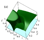
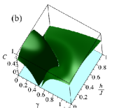
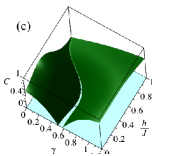
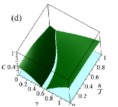
Figure 5: (Color Online) Thermal entanglement deterioration as a function of $\gamma$ and $h/J$ when temperature increases and fixed $J_{0}/J=-0.3$ and $J_{z}/J=0.3$. (a) $T/J=0.02$. (b) $T/J=0.04$. (c) $T/J=0.08$. (d) $T/J=0.16$.

For the purpose to give a more detailed behavior of the concurrence as a function of $\gamma$ and $h/J$. In figure 5 is illustrated the concurrence as a sequence of higher temperature than figure 4(a), assuming the concurrence for same fixed parameters $J_{0}/J=-0.3$ and $J_{z}/J=0.3$. In fig.5(a) the thermal entanglement is illustrated at $T/J=0.02$, basically still remains the entangled region (figure 4(a)) and displaying the change of disentangled region. In fig.5(b) is illustrated for $T/J=0.04$, showing how the entangled region "deteriorate" and how the disentangled region is modified. Similarly in fig.5(c) is illustrated for $T/J=0.08$, where entangled region becoming increasingly deteriorate. Lastly in fig.5(d) is shown for $T/J=0.16$, at this temperature the entangled region was highly modified compared to that figure 4(a), showing only a nearly straight valley. In summary, we illustrate how the thermal entanglement "deteriorate" (vanishes) as far as the temperature increases.

IV.1 Threshold temperature

We follow a similar definition of the critical temperature for the threshold temperature $T_{th}$, such as disorder-order-disorder (or inverse) sequences of transition (reentrant phenomenon) have been observed in many systems. The reentrant phase transition has been observed for the first time in polymer gels katayama , frustrated spin-gas model berker , Rochelle salts levitskii , and a predator - prey model Han . Quantum reentrant phase transitions (disentangled (D) - entangled (E) - disentangled (D) - entangled (E) - disentangled (D) regions) of the concurrence versus magnetic field has been obtains noticed in Lipkin-Meshkov-Glick model Morrison .

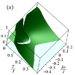
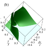
Figure 6: (Color Online) Thermal entanglement deterioration when temperature increases. (a) For $J_{z}/J=0$, $\gamma=0.95$ and $h/J=0.27$. (b) For $J_{z}/J=0.3$, $\gamma=0.6$ and $h/J=0.35$.

In figure 6(a) is illustrated the concurrence as a function of $T/J$ and $J_{0}/J$ assuming a fixed value $J_{z}/J=0$, $\gamma=0.95$ and $h/J=0.27$, here we can observe how the concurrence vanishes and for a higher temperature arise a thermal entanglement. Thereafter, the entanglement for even a higher temperature disappears altogether. In figure 6(b) is depicted the concurrence as a function of $T/J$ and $J_{0}/J$ assuming a fixed value $J_{z}/J=0.3$, $\gamma=0.6$ $h/J=0.35$, we can also observe, how the concurrence vanishes for higher temperature and for a bit higher temperature emerges a small thermal entanglement, hereafter the entanglement for higher temperature disappears definitely.

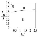
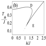
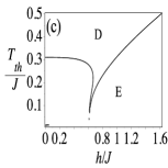
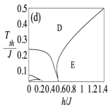
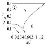
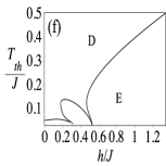
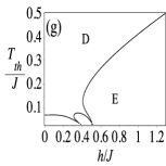
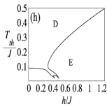
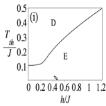
Figure 7: Threshold temperature limiting entangled (E) and disentangled (D) region as a function of magnetic field, assuming fixed parameters values $J_{0}/J=-0.3$ and $J_{z}/J$=0.3, for several values of XY-anisotropy $\gamma$. (a) $\gamma=0$, (b) $\gamma=0.1$, (c) $\gamma=0.4$, (d) $\gamma=0.5$, (e) $\gamma=0.53$, (f) $\gamma=0.535$, (g) $\gamma=0.56$, (h) $\gamma=0.585$, (i) $\gamma=0.6$.

In figure 7 is illustrated the threshold temperature $T_{th}$ as a function of the magnetic field for several values of XY-anisotropy $\gamma$. The curves mean the threshold temperature, limiting entangled (E) and disentangled (D) region as a function of the magnetic field, assuming fixed parameters values $J_{0}/J=-0.3$ and $J_{z}/J$=0.3, for several values of XY-anisotropy $\gamma$. Fig. 7(a) for $\gamma=0$, is observed the threshold temperature upper region corresponds to entangled (E) and bottom region corresponds to disentangled (D) region. (b) For $\gamma=0.1$, we observe a rise of threshold temperature $T_{th}$ for the left side curve. From fig.7(a-b), we observe those threshold temperature curves are highly sensitive for $\gamma\neq 0$, because the entanglement are extremely small close to threshold temperature. (c) For $\gamma=0.4$, the reentrance temperature decreases and also rise a small disentangled region below entangled region for $h/J\lesssim 0.6$. (d) For $\gamma=0.5$, the disentangled region increases and still remains the reentrance temperature $T_{th}$ for the right side curve. (e) For $\gamma=0.53$, the entangled region shrinks even more and we can observe two quite interesting reentrance temperature. (f) Increasing little bit the XY-anisotropy $\gamma=0.535$, we observe how the reentrance temperature modify. (g) Despite being similar to the previous plot for $\gamma=0.56$, is illustrated how the reentrance temperature vanishes. (h) For $\gamma=0.585$, the threshold temperature behaves similarly to the previous plot (g). (i) For $\gamma=0.6$ the typical reentrance temperature vanishes, despite there is a small isolated disentangled region.

V Conclusions

In summary, we have presented a detailed study of the spin-1/2 Ising-XYZ chain on diamond structure, which is an exactly solvable model through the decoration transformation and transfer matrix approach. The phase diagram of ground state energy was discussed, displaying frustrated region and the pairwise thermal entanglement between two Heisenberg spin. It is noteworthy that at zero temperature, there are non-zero concurrence in a vast region for the Hamiltonian parameter, only in the limiting case the entanglement vanishes for some regions such as the case of Ising-XXZ diamond chainspra . Due to XY-anisotropy the Hamiltonian, we found quite interesting behavior for the thermal entanglement, such as the presence of more than one threshold temperature, this phenomenon is influenced by XY-anisotropy ($\gamma$), which means the entanglement vanishes at threshold temperature and for higher temperature arise the thermal entanglement again, and finally, for an even higher temperature, the entanglement vanishes definitely. It is worth to emphasize, a similar result was discussed in referenceG. Rigolin ; Zhou-Song , but for only two qubits, and here we propose how this property can be possible measured in condensed matter materials.

References

- (1) K. M. OConnor and W. K. Wootters, Phys. Rev. A 63, 052302 (2001); Y. Sun, Y. Chen and H. Chen, Phys. Rev. A 68, 044301 (2003).
- (2) G. L. Kamta and A. F. Starace, Phys. Rev. Lett. 88, 107901 (2002).
- (3) F. Verstraete, M.A. Martin-Delgado, J.I. Cirac, Phys. Rev. Lett. 92, 087201 (2004).
- (4) M. Popp, F. Verstraete, M. A. Martin-Delgado, J. I. Cirac, Phys. Rev. A 71, 042306 (2005) .
- (5) J. J. Garcia-Ripoll, M. A. Martin-Delgado, J. I. Cirac, Phys. Rev. Lett. 93, 250405 (2004).
- (6) A. Honecker, S. Hu, R. Peters J. Ritcher, J. Phys.: Condens. Matter 23, 164211 (2011).
- (7) L. Canova, J. Strecka, M. Jascur, J. Phys.: Condens. Matter 18, 4967 (2006).
- (8) B. M. Lisnii, Ukrainian Journal of Physics 56, 1237 (2011).
- (9) O. Rojas, S.M. de Souza, V. Ohanyan, M. Khurshudyan, Phys. Rev. B 83 , 094430 (2011).
- (10) J.S. Valverde, O. Rojas, S.M. de Souza, J. Phys. Condens. Matter 20, 345208 (2008); O. Rojas, S.M. de Souza, Phys. Lett. A 375, 1295 (2011).
- (11) K. C. Rule et al., Phys. Rev. Lett. 100, 117202 (2008).
- (12) H. Kikuchi et al., Phys. Rev. Lett. 94, 227201 (2005); H. Kikuchi et al., Prog. Theor. Phys. Suppl. 159, 1 (2005).
- (13) N. S. Ananikian, L. N. Ananikyan, L. A. Chakhmakhchyan and O. Rojas, J. Phys.: Condens. Matter 24, 256001 (2012).
- (14) L. Chakhmakhchyan, N. Ananikian, L. Ananikyan and C. Burdik, J. Phys: Conf. Series 343, 012022 (2012).
- (15) X. Wang, Phys. Rev. A 66, 044305 (2002).
- (16) M. C. Arnesen, S. Bose and V. Vedral, Phys. Rev. Lett. 87, 017901 (2001).
- (17) Xiaoguang Wang, Phys. Rev. A 66, 034302 (2002) .
- (18) G. Rigolin, Int. J. Quant. Inf. 2, 393 (2004).
- (19) L. Zhou, H. S. Song, Y. Q. Guo and C. Li, Phys. Rev. Lett. A 68, 024301 (2003).
- (20) M. Rojas, S. M. de Souza, O. Rojas, Phys. Rev. A 89, 032336 (2014).
- (21) N. Ananikian, H. Lazaryan, M, Nalbandyan, Eur. Phys. J. B 85, 223 (2012).
- (22) I. Syozi, Prog. Theor. Phys. 6, 341 (1951).
- (23) M. Fisher, Phys. Rev. 113, 969 (1959).
- (24) O. Rojas, J. S. Valverde, S. M. de Souza, Physica A 388, 1419 (2009); O. Rojas, S. M. de Souza, J. Phys. A: Math. Theor. 44, 245001 (2011).
- (25) J Strečka, Phys. Lett. A 374, 3718 (2010).
- (26) R.J. Baxter, Exactly Solved Models in Statistical Mechanics, (Academic Press, New York, 1982).
- (27) W. K. Wootters, Phys. Rev. Lett. 80, 2245 (1998).
- (28) D. J. Bukman, G. An, and J. M. J. van Leeuwen, Phys. Rev. B 43, 13352 (1991).
- (29) L. Amico, A. Osterloh, F. Plastina, R. Fazio and G. M. Palma, Phys. Rev. A 69, 022304 (2004).
- (30) O. Rojas, M. Rojas, N. S. Ananikian and S. M. de Souza, Phys. Rev. A 86, 042330 (2012).
- (31) S. Katayama, Y. Hirokawa, and T. Tanaka, Macromolecules 17, 2641 (1984); S. Hirotsu, Y. Hirokawa, and T. Tanaka, J. Chem. Phys. 87, 1392 (1987).
- (32) A.N. Berker and J.S. Walker, Phys. Rev. Lett. 47, 1469 (1981).
- (33) R. R. Levitskii, I. R. Zachek, A. P. Moina, and A. Ya. Andrusyk, Condens. Matter Phys. 97, 111 (2004).
- (34) S.-G. Han, S.-C.Park, and B. J. Kim, Phys. Rev. E 79, 066114 (2009).
- (35) S. Morrison and A. S. Parkins, Phys. Rev. Lett. 100, 040403 (2008).