Sticky particles and stochastic flows

Abstract.

Gawȩdzki and Horvai have studied a model for the motion of particles carried in a turbulent fluid and shown that in a limiting regime with low levels of viscosity and molecular diffusivity, pairs of particles exhibit the phenomena of stickiness when they meet. In this paper we characterise the motion of an arbitrary number of particles in a simplified version of their model.

1. Introduction

The motivation for this paper comes from a work by Gawȩdzki and Horvai, [gh], in which the authors study a model for the motion of particles carried in a turbulent fluid. The trajectories of two distinct particles $\bigl{(}X_{1}(t),t\geq 0\bigr{)}$ and $\bigl{(}X_{2}(t),t\geq 0\bigr{)}$ are each described by a Brownian motion in ${\mathbf{R}}^{d}$ with a covariance of the form

(1) $$\langle X_{1},X_{2}\rangle(t)=\int_{0}^{t}\psi\bigl{(}X_{1}(s)-X_{2}(s)\bigr{)}ds.$$

The $d\times d$ matrix valued function $\psi$ is invariant under the natural action of the orthogonal group and consequently the inter-particle distance $\|X_{1}(t)-X_{2}(t)\|$ is a diffusion process on ${\mathbf{R}}_{+}$. For different choices of the covariance function $\psi$, different qualitative behaviours are observed, and these correspond to different boundary conditions at $0$ for the diffusion describing the inter-particle distance. See also Le Jan and Raimond [lejan1] for a description of these phases. Gawȩdzki and Horvai study the case where $0$ is both a entrance and exit boundary point, and the function $\psi$ is not smooth at the origin. They then introduce a viscosity effect acting at small scales by replacing $\psi$ by a smooth covariance function obtained by smoothing $\psi$ in a neighbourhood of the origin. Particles moving in this regularized flow never meet, and $0$ is now a natural boundary point for the diffusion describing the inter-particle distance. They then further vary the model and consider particles whose motion is affected by molecular diffusivity, modelled by adding, for each particle, a small independent Brownian perturbation to the motion of the flow. If the additional diffusivity and the scale at which viscosity acts both are taken to zero in an appropriate balance then Gawȩdzki and Horvai show that the inter-particle distance $\|X^{(1)}(t)-X^{(2)}(t)\|$ converges to a diffusion on ${\mathbf{R}}_{+}$ with the boundary point being sticky: that is a regular boundary point at which the diffusion spends a strictly positive amount of time.

Sticky boundary behaviour was first identified by Feller, as described in the article [pes]. Subsequently the process which is a Brownian motion on ${\mathbf{R}}_{+}$ with a sticky boundary at $0$ was studied as an example of a stochastic differential equation with no strong solution, see Chitashvili, [ch] and Warren [w1], and recent work by Engelbert and Peskir [ep] and Bass [bass]. Stochastic flows in which the inter-particle distance evolves as a sticky Brownian motion have been studied by Le Jan and Lemaire [lejan3], by Howitt and Warren [hw1] and [hw2], and by Schertzer, Sun and Swart, [sss].

In this paper we study a simplification of the Gawȩdzki-Horvai model. Our goal is to address, in this simplified setting, the question raised by Gawȩdzki and Horvai of characterizing the behaviour of $N$ particles. We take the dimension of the underlying space to be $d=1$, and the motion of distinct particles, in the absence of viscosity or molecular diffusivity, to be given by Brownian motions which are independent of one another until the particles meet.

Let $\psi$ be a real-valued, smooth, positive definite function on ${\mathbf{R}}$, satisfying $\psi(0)=1$, $|\psi(x)|<1$ for $x\neq 0$, and $\psi(x)\rightarrow 0$ as $|x|\rightarrow\infty$. Define the constant $a$, which we assume is strictly positive, via

(2) $$\frac{1-\psi(x)}{x^{2}}\rightarrow a^{2}\text{ as }x\rightarrow 0.$$

For each $n$ there exists a smooth flow of Brownian motions associated with the scaled covariance function $\psi(nx)$, the $N$ point motion of which has generator

(3) $$\frac{1}{2}\sum_{i,j}\psi\bigl{(}n(x_{i}-x_{j})\bigr{)})\frac{\partial^{2}}{\partial x_{i}x_{j}}.$$

As $n$ tends to infinity the covariance functions $\psi(nx)$ converge to the singular covariance $1_{0}(x)$, and correspondingly, the $N$-point motions associated with the flows converge to systems of coalescing Brownian motions.

Fix a constant $b>0$ and for $n\geq 1$, we define generators

(4) $${\mathcal{G}}^{N,n}=\frac{1}{2}\sum_{i,j}\psi\bigl{(}n(x_{i}-x_{j})\bigr{)}\frac{\partial^{2}}{\partial x_{i}x_{j}}+\frac{b^{2}}{2n^{2}}\sum_{i}\frac{\partial^{2}}{\partial x_{i}^{2}}$$

which are perturbations of the generators (3) by addition of the Laplacian with co-efficient $b^{2}/2n^{2}$. This works against coalescence by giving each particle in the flow a small amount of independent diffusivity. As a consequence paths of particles in the flow can cross and the $N$-point motions are no longer associated with flow of maps.

The two effects: approximating a coalescing flow by smooth flows, and adding diffusivity, are in balance as we pass to the limit, as can be seen by the following analysis of the $2$-point motion. Let $(X_{1},X_{2})$ be the two point motion with generator ${\mathcal{G}}^{2,n}$. It is enough to consider the difference $Z(t)=X_{1}-X_{2}(t)$ which is a diffusion on the real line in natural scale and with speed measure

(5) $$m_{n}(dz)=\frac{dz}{1+b^{2}n^{-2}-\psi(nz)}$$

As $n$ tends to infinity $m_{n}$ weakly converges to the measure $m(dz)=dz+\theta^{-1}\delta_{0}(dz)$ where the constant $\theta$ is given by

(6) $$\theta^{-1}=\int_{-\infty}^{\infty}\frac{dz}{b^{2}+a^{2}z^{2}}=\frac{\pi}{ab}.$$

Thus the limiting diffusion describing $|X_{1}-X_{2}|$ is a sticky Brownian with the parameter $\theta$ describing the degree of stickiness at $0$, and the limit of the two point motion is determined by this, together with $X_{1}$ and $X_{2}$ each being Brownian motions.

This leaves open the limiting behaviour of the perturbed $N$-point motions for $N\geq 3$. Consistent families of diffusions in ${\mathbf{R}}^{N}$ whose components are Brownian motions evolving as independent Brownian motions whenever they are unequal were studied in [hw1]. For such processes there are times at which many co-ordinates co-incide and it is necessary to describe the sticky behaviour at such times. This is specified by families of of non-negative co-efficients $(\theta(k:l);k,l\geq 1)$. Thinking of the $N$-point motion as a system of $N$ particles $\theta(k:l)$ gives the rate, in an excursion theoretic sense, at which a clump of $k+l$ particles separates into two clumps one consisting of $k$ particles and the other of $l$ particles. The result of this paper is the following identification of these co-efficients for our model.

Theorem 1.

The $N$ point motions with generators ${\mathcal{G}}^{N,n}$ converge in law as $n$ tends to infinity to a family of sticky Brownian motions associated to the family of parameters $(\theta(k:l);k,l\geq 1)$ given by

$$\theta(k:l)=\frac{ab}{2\sqrt{\pi}}\int_{\mathbf{R}}\int_{{\mathbf{R}}^{k+l}}\frac{e^{-\|x\|^{2}/2}}{(2\pi)^{(k+l)/2}}{\mathbf{1}}(x_{1},x_{2},\ldots x_{k}<z<x_{k+1},\ldots,x_{k+l})dxdz$$

The form of the parameters $\theta(k:l)$ given in this result is highly suggestive of the underlying mechanisms at work. The variables $x_{1},\dots,x_{k+l}$ chosen according to a Gaussian measure can be thought of as the positions of a cluster of $k+l$ particles experiencing independent diffusivity, and the variable $z$ represents a “singularity” in the underlying flow that causes the cluster to separate into two. Of course this is far from being rigorous.

To give Theorem 1 a precise meaning we must specify the law of the family of sticky Brownian motions associated to the family of parameters $(\theta(k:l);k,l\geq 1)$. We do this by means of a well-posed martingale problem, following [hw1].

Suppose $\bigl{(}\theta(k:l);k,l\geq 1)$ is a family of nonnegative parameters satisfying the consistency property

(7) $$\theta(k:l)=\theta(k+1:l)+\theta(k:l+1)$$

For our purposes in this paper we may also assume the symmetry $\theta(k:)=\theta(l:k)$. We now recall the main result from [hw1] concerning the characterization of consistent families of sticky Brownian motions.

We begin by partitioning ${\mathbf{R}}^{N}$ into cells. A cell $E\subset{\mathbf{R}}^{N}$ is determined by some weak total ordering $\preceq$ of the $\{1,2,\ldots N\}$ via

(8) $$E=\{x\in{\mathbf{R}}^{N}:x_{i}\leq x_{j}\text{ if and only if }i\preceq j\}.$$

Thus $\{x\in{\mathbf{R}}^{3}:x_{1}=x_{2}=x_{3}\}$, $\{x\in{\mathbf{R}}^{3}:x_{1}<x_{2}=x_{3}\}$ and $\{x\in{\mathbf{R}}^{3}:x_{1}>x_{2}>x_{3}\}$ are three of the thirteen distinct cells into which ${\mathbf{R}}^{3}$ is partitioned.

Suppose that $I$ and $J$ are disjoint subsets of $\{1,2,\ldots,N\}$ with both $I$ and $J$ non-empty. With such a pair we associate a vector $v=v_{I,J}$ belonging to ${\mathbf{R}}^{N}$ with components given by

(9) $$v_{i}=\begin{cases}0&\text{ if $i\not\in I\cup J$,}\\ +1&\text{ if $i\in I$,}\\ -1&\text{ if $i\in J$.}\end{cases}$$

We associate with each point $x\in{\mathbf{R}}^{N}$ certain vectors of this form. To this end note that each point $x\in{\mathbf{R}}^{N}$ determines a partition $\pi(x)$ of $\{1,2,\ldots N\}$ such that $i$ and $j$ belong to the same component of $\pi(x)$ if and only if $x_{i}=x_{j}$. Then to each point $x\in{\mathbf{R}}^{N}$ we associate the set of vectors, denoted by ${\mathcal{V}}(x)$, which consists of every vector of the form $v=v_{IJ}$ where $I\cup J$ forms one component of the partition $\pi(x)$.

Let $L_{N}$ be the space of real-valued functions defined on ${\mathbf{R}}^{N}$ which are continuous, and whose restriction to each cell is given by a linear function. Given a set of parameters $\bigl{(}\theta(k:l);k,l\geq 0\bigr{)}$ we define the operator ${\mathcal{A}}^{\theta}_{N}$ from $L_{N}$ to the space of real valued functions on ${\mathbf{R}}^{N}$ which are constant on each cell by

(10) $${\mathcal{A}}^{\theta}_{N}f(x)=\sum_{v\in{\mathcal{V}}(x)}\theta(v)\nabla_{v}f(x).$$

Here on the righthandside $\theta(v)=\theta(k:l)$ where $k=|I|$ is the number of elements in $I$ and $l=|J|$ is the number of elements in $J$ for $I$ and $J$ determined by $v=v_{IJ}$. $\nabla_{v}f(x)$ denotes the (one-sided) gradient of $f$ in the direction $v$ at the point $x$, that is

(11) $$\nabla_{v}f(x)=\lim_{\epsilon\downarrow 0}\frac{1}{\epsilon}\bigl{(}f(x+\epsilon v)-f(x)\bigr{)}.$$

We say an ${\mathbf{R}}^{N}$-valued stochastic process $\bigl{(}X(t);t\geq 0\bigr{)}$ solves the ${\mathcal{A}}^{\theta}_{N}$-martingale problem if for each $f\in L_{N}$,

$$f\bigl{(}X(t)\bigr{)}-\int_{0}^{t}{\mathcal{A}}_{N}^{\theta}f\bigl{(}X(s)\bigr{)}ds\text{ is a martingale,}$$

relative to some common filtration, and the bracket between co-ordinates $X_{i}$ and $X_{j}$ is given by

$$\langle X_{i},X_{j}\rangle(t)=\int_{0}^{t}{\mathbf{1}}{(X_{i}(s)=X_{j}(s))}ds\qquad\text{ for }t\geq 0.$$

In particular $\langle X_{i}\rangle(t)=t$. According to the main result of [hw1], for any given starting point $x\in{\mathbf{R}^{N}}$, a solution to the ${\mathcal{A}}^{\theta}_{N}$-martingale problem exists and its law is unique. It is a process with this law that we refer to as a family of $N$ sticky Brownian motions associated with the parameters $\bigl{(}\theta(k:l);k,l\geq 1)$.

2. Heuristic derivation of exit probabilities

Let us write $\bigl{(}X(t);t\geq 0\bigr{)}$ for the co-ordinate process on $N$ dimensional path space, and we will write $\hat{X}(t)$ for the projection $X(t)$ onto the hyperplane ${\mathbf{R}}^{N}_{0}=\{x\in{\mathbf{R}}^{N}:\sum x_{i}=0\}$. Suppose that $X$ when governed by a probability measure ${\mathbf{P}}^{N,\theta}_{x}$ evolves as the family of $N$ mutually sticky Brownian motions associated with a parameters $\theta=(\theta(k:l);k,l\geq 1)$ started from $x\in{\mathbf{R}}^{N}$. Consider, for $\epsilon>0$, the neighbourhood $D(\epsilon)$ of the origin $0$ in ${\mathbf{R}}^{N}_{0}$ given by

(12) $$D(\epsilon)=\{x\in{\mathbf{R}}^{N}_{0}:\max_{i,j}(x_{i}-x_{j})\leq\epsilon\}.$$

We know from [hw1] that the exit distribution of $\hat{X}$ from $D(\epsilon)$ can, for small $\epsilon$, be described in terms of the $\theta(k:l)$ parameters. In fact if $T(\epsilon)$ denotes the first time that $\hat{X}$ leaves this set, we have

(13) $$\lim_{\epsilon\downarrow 0}\frac{1}{\epsilon}{\mathbf{E}}^{N,\theta}_{0}\bigl{[}T(\epsilon)\bigr{]}=\frac{1}{2\sum_{k=1}^{N-1}{N\choose k}\theta(k:N-k)},$$

and, for each cell $E$ that corresponds to a (ordered) partition of $\{1,.2,\ldots,N\}$ into two parts having sizes $k$ and $l=N-k$,

(14) $$\lim_{\epsilon\downarrow 0}{\mathbf{P}}^{N,\theta}_{0}\bigl{(}X(T(\epsilon))\in E)=\frac{\theta(k:l)}{\sum_{k=1}^{N-1}{N\choose k}\theta(k:N-k)}$$

Notice how this is consistent with the idea that $\theta(k,N-k)$ describes the rate at which a cluster of $N$ particles splits.

In view of these observations on the behaviour of sticky diffusions we can reasonably expect to be able to identify the parameters $\theta(k:l)$ arising in the limiting behaviour of our $N$ point motions with generators (4) by investigating how these processes, for $n$ large, leave neighbourhoods of the origin. Interestingly very close to the origin, at distances of the order $1/n^{2}$, the $N$ point motions are spherically symmetric, but at larger distances a coalescence effect leads to exit distributions concentrated on points corresponding to the cluster of particles splitting into two subclusters.

We will suppose that $X$ when governed by probability measures ${\mathbf{P}}^{N,n}_{x}$ evolves as a diffusion with generator ${\mathcal{G}}^{N,n}$ starting from $x\in{\mathbf{R}}^{N}$. Notice that the generators ${\mathcal{G}}^{N,n}$ are invariant under shifts $(x_{1},x_{2},\ldots x_{N})\mapsto(x_{1}+h,x_{2}+h,\ldots x_{N}+h)$, and consequently the projection $\hat{X}(t)$ of $X(t)$ is a diffusion also. In view of (13) and (14) it is natural to study the exit time and distribution of $\hat{X}$ from $D(\epsilon)$ under ${\mathbf{P}}^{N,n}_{0}$ in order to determine the parameters $\theta(k:l)$ associated with the limiting $N$ point motion. We will estimate the exit distribution (non-rigorously) by approximating the behaviour of $\hat{X}$ on two different scales.

Let $B(r)$ denote the ball of radius $r$ in ${\mathbf{R}}^{N}_{0}$,

$$B(r)=\{x\in{\mathbf{R}}^{N}_{0}:\|x\|\leq r\}.$$

Now, for a fixed small $\epsilon>0$, the map $x\mapsto\psi(x)$ is approximately quadratic for $x\in(-\epsilon,\epsilon)$ and we use this to approximate the covariance matrix of $\hat{X}$ in the ball $B(\epsilon/n)$. Observe that if the matrix $A$ has entries $1-a^{2}(x_{i}-x_{j})^{2}$ then for vectors $u,v\in{\mathbf{R}}^{N}_{0}$ we have $(u,Av)=2a^{2}(u,x)(v,x)$. Consequently we can approximate $\hat{X}$ under ${\mathbf{P}}^{N,n}$ within the ball $B(\epsilon/n)$ as $(n^{-2}Z(n^{2}t);t\geq 0)$ where $Z$ is a diffusion with generator ${\mathcal{H}}^{N}$ given by, in spherical co-ordinates in ${\mathbf{R}}^{N}_{0}$,

(15) $${\mathcal{H}}^{N}=a^{2}r^{2}\frac{\partial^{2}}{\partial r^{2}}+\frac{b^{2}}{2}\nabla^{2}=\left(\frac{b^{2}}{2}+a^{2}r^{2}\right)\frac{\partial^{2}}{\partial r^{2}}+\frac{(N-2)b^{2}}{2r}\frac{\partial}{\partial r}+\frac{b^{2}}{2r^{2}}\Delta_{S^{N-2}}.$$

In particular, the rescaled radial part of $\hat{X}$ is approximated as a diffusion on $(0,\infty)$ with generator

(16) $${\mathcal{H}}^{N}_{\text{rad}}=\left(\frac{b^{2}}{2}+a^{2}r^{2}\right)\frac{d^{2}}{dr^{2}}+\frac{(N-2)b^{2}}{2r}\frac{d}{dr}.$$

The expected time taken for this diffusion to first reach a level $r$ when started from $0$ is equal to $f_{0}(r)$ where $f_{0}$ is the increasing solution to

$${\mathcal{H}}^{N}_{\text{rad}}f_{0}=1,\qquad\qquad f_{0}(0)=0.$$

The function $f_{0}(r)$ is asymptotically equal to $r/(\gamma ab)$, see [w2], where

(17) $$\gamma=\sqrt{\frac{2}{\pi}}\frac{\Gamma(N/2)}{\Gamma((N-1)/2)}=\frac{1}{\sqrt{\pi}}\int_{{\mathbf{R}}^{N-1}}\frac{\|x\|e^{-\|x\|^{2}/2}}{(2\pi)^{(N-1)/2}}\;dx.$$

Thus we have the estimate

(18) $${\mathbf{E}}_{0}^{N,n}[\text{exit time from $B(\epsilon/n)$ }]\approx\frac{\epsilon}{n\gamma ab}.$$

Moreover, because of the spherical symmetry of ${\mathcal{H}}^{N}$, the exit distribution from this ball is the uniform measure on sphere.

We next consider $\hat{X}$ started from a point $x$ on the sphere of radius $\epsilon/n$ which we will assume has distinct co-ordinates. Let $\sigma$ be the permutation so that $x_{\sigma(1)}>x_{\sigma(2)}>\cdots>x_{\sigma(N)}$, and denote by $x^{\sigma}$ the vector $(x_{\sigma(1)},x_{\sigma(2)},\cdots,x_{\sigma(N)})$ . Our second approximation applies to $\hat{X}$ until it first leaves the domain $D(\epsilon)\setminus D(1/(\epsilon n^{2}))$. If two particles come close to each other, then they have a negligible probability of separating by a significant distance prior to the exit time $\tau$ from the domain. Thus we can treat $\hat{X}$ similarly to (the projection to ${\mathbf{R}}^{N}_{0}$) of a system of $N$ coalescing Brownian motions. In particular this means that if $\hat{X}$ exits via the outer part of the boundary then it does so with $\hat{X}^{\sigma}_{1}(\tau)-\hat{X}^{\sigma}_{N}(\tau)\approx\epsilon$. Consequently applying the optional stopping Theorem to the martingale $\hat{X}^{\sigma}_{1}(t)-\hat{X}^{\sigma}_{N}(t)$ gives rise to the estimate

(19) $${\mathbf{P}}^{N,n}_{x}\bigl{(}\hat{X}\text{ exits $D(\epsilon)\setminus D(1/(\epsilon n^{2}))$ via the outer boundary }\bigr{)}\approx\frac{x^{\sigma}_{1}-x^{\sigma}_{N}}{\epsilon}.$$

Moreover if $\hat{X}$ does exit via the outer boundary then as it does so there are only two clusters of particles (see Lemma 6 for the corresponding statement about coalescing Brownian motion), and applying the optional stopping Theorem to $\hat{X}^{\sigma}_{k}(t)-\hat{X}^{\sigma}_{k+1}(t)$ gives

(20) $${\mathbf{P}}^{N,n}_{x}\bigl{(}\hat{X}^{\sigma}_{i}(\tau)-\hat{X}^{\sigma}_{i+1}(\tau)\approx 0\text{ for $i\neq k$, }\hat{X}^{\sigma}_{k}(\tau)-\hat{X}^{\sigma}_{k+1}(\tau)\approx\epsilon\bigr{)}\approx\frac{x^{\sigma}_{k}-x^{\sigma}_{k+1}}{\epsilon}.$$

We now make use of a renewal argument. The diffusion with generator (15) is ergodic, and consequently we conclude that the process $\hat{X}$ spends all but a negligible amount of time at a distance of order $1/n^{2}$ from the origin prior to exiting $D(\epsilon)$. From this inner region it makes excursions to the sphere of radius $\epsilon/n$ and, each time it does, it has a small probability of exiting $D(\epsilon)$ rather than returning to the inner region. When it does return to distances of order $1/n^{2}$ we can assume by mixing that it is starts afresh and forgets its history. Thus $\hat{X}$ makes approximately a geometrically distributed number of excursions to the sphere of radius $\epsilon/n$ before exiting $D(\epsilon)$, and we conclude, neglecting the time spent outside the ball $B(\epsilon/n)$, that the expected time to exit $D(\epsilon)$ is estimated by

(21) $$\frac{{\mathbf{E}}_{0}^{N,n}[T_{B(\epsilon/n)}]}{{\mathbf{E}}_{0}^{N,n}\bigl{[}{\mathbf{P}}^{N,n}_{X(T_{B(\epsilon/n)})}\bigl{(}\hat{X}\text{ exits $D(\epsilon)\setminus D(1/(\epsilon n^{2}))$ via the outer boundary }\bigr{)}\bigr{]}},$$

where $T_{B(\epsilon/n)}$ denotes the first time of exiting the ball $B(\epsilon/n)$. Similarly we estimate that the probability of exiting $D(\epsilon)$ at time $T_{D(\epsilon)}$ with $\hat{X}_{i+1}(T_{D(\epsilon)})-\hat{X}_{i}(T_{D(\epsilon)})\approx 0$ for all $i\neq k$ and $\hat{X}_{k+1}(T_{D(\epsilon)})-\hat{X}_{k}(T_{D(\epsilon)})\approx\epsilon$ is approximately

(22) $$\frac{{\mathbf{E}}_{0}^{N,n}\bigl{[}{\mathbf{P}}^{N,n}_{X(T_{B(\epsilon/n)})}\bigl{(}\hat{X}_{i}(\tau)-\hat{X}_{i+1}(\tau)\approx 0\text{ for $i\neq k$, }\hat{X}_{k}(\tau)-\hat{X}_{k+1}(\tau)\approx\epsilon\bigr{)}\bigr{]}}{{\mathbf{E}}_{0}^{N,n}\bigl{[}{\mathbf{P}}^{N,n}_{X(T_{B(\epsilon/n)})}\bigl{(}\hat{X}\text{ exits $D(\epsilon)\setminus D(1/(\epsilon n^{2}))$ via the outer boundary }\bigr{)}\bigr{]}},$$

where, as previously, $\tau$ is the exit time of $D(\epsilon)\setminus D(1/(\epsilon n^{2}))$. Thus, in view of (13) and (14), and taking the cell $E=\{x_{1}=x_{2}=\ldots=x_{k}<x_{k+1}=x_{k+2}=\ldots=x_{N}\}$, we guess that the parameter $\theta(k:N-k)$ associated with a limiting $N$-point motion should be equal to the limit as $n$ tends to infinity and $\epsilon$ tends to zero of

(23) $$\frac{\epsilon\times{\mathbf{E}}_{0}^{N,n}\bigl{[}{\mathbf{P}}^{N,n}_{X(T_{B(\epsilon/n)})}\bigl{(}\hat{X}_{i}(\tau)-\hat{X}_{i+1}(\tau)\approx 0\text{ for $i\neq k$, }\hat{X}_{k}(\tau)-\hat{X}_{k+1}(\tau)\approx\epsilon\bigr{)}\bigr{]}}{2{\mathbf{E}}_{0}^{N,n}[T_{B(\epsilon/n)}]}$$

Substituting in our estimates from (18) and (20) and using the fact that the exit distribution from $B(\epsilon/n)$ is uniform we arrive at

(24) $$\frac{\gamma ab}{2}\int_{S^{N-2}}\bigl{(}\min_{1\leq i\leq k}z_{i}-\max_{k+1\leq i\leq N}z_{i})\bigr{)}^{+}dz.$$

in which the integral over the unit sphere $S^{N-2}\subset{\mathbf{R}}^{N}_{0}$ is taken with respect to Lebesgue measure on the sphere normalized so $\int_{S^{N-2}}dz=1$. When we rewrite the spherical integral as a Gaussian integral this agrees the value given in Theorem 1.

3. Proof of main result

In view of the characterization of a family of sticky Brownian motions by the ${\mathcal{A}}^{\theta}_{N}$-martingale problem, it is a natural strategy to prove Theorem 1 by considering smooth approximations $f_{n}$ to a given function $f\in L_{N}$ and to derive, using weak convergence, from the martingale property, under ${\mathbf{P}}^{N,n}$, of

(25) $$f_{n}(X(t))-\int_{0}^{t}{\mathcal{G}}^{N,n}f_{n}(X(s))ds$$

that

$$f(X(t))-\int_{0}^{t}{\mathcal{A}}^{\theta}_{N}f(X(s))ds,$$

is a martingale under ${\mathbf{P}}^{N,\theta}$. There are difficulties to be overcome in pursuing this which arise because ${\mathcal{A}}^{\theta}_{N}f$ is not continuous. A key step is to establish the weaker statement described in the following lemma, which gives information about how the limiting process leaves the main diagonal $D=\{x\in{\mathbf{R}}^{N}:x_{1}=x_{2}=\ldots=x_{N}\}$. Let $L_{N}^{0}$ denote the subspace of $L_{N}$ containing those functions which are invariant under shifts $(x_{1},x_{2},\ldots,x_{n})\mapsto(x_{1}+h,x_{2}+h,\ldots,x_{n}+h)$, and consequently identically equal to $0$ on $D$.

Lemma 2.

Fix $x\in{\mathbf{R}}^{N}$, and suppose that ${\mathbf{P}}_{x}$ is a subsequencial limit of the family of probability measures $\bigl{(}{\mathbf{P}}_{x}^{N,n};n\geq 1\bigr{)}$. Then for any convex $f\in L^{N}_{0}$,

$$Z^{f}(t)=f(X(t))-{\mathcal{A}}^{\theta}_{N}f(0)\int_{0}^{t}{\mathbf{1}}(X(s)\in D)ds$$

is a submartingale under ${\mathbf{P}}_{x}$, where the family of parameters $\theta$ are specified as in Theorem 1.

We will prove this lemma by applying weak convergence to ${\mathbf{P}}^{N,n}$ martingales given at (25). But it turns out that we must carefully select suitable smooth approximations $f_{n}$. In fact we will choose $f_{n}(x)=n^{2}g(n^{-2}x)$ where the function $g$ is determined according to the next proposition which is adapted from [w2].

Recall that the generators ${\mathcal{G}}^{N,n}$, rescaled and restricted to ${\mathbf{R}}^{N}_{0}$, converge to ${\mathcal{H}}^{N}$ given by(15). The constant $gamma$ was defined at (17).

Proposition 3.

Let $f:S^{N-2}\rightarrow{\mathbf{R}}$ be a square integral function on the unit sphere $S^{N-2}\subset{\mathbf{R}}^{N-1}_{0}$. Let

$$c=c(f)=\gamma ab\int_{S^{N-2}}f(z)dz$$

where the integral is with respect to normalized Lebesgue measure on the sphere. There exists a unique solution to

$${\mathcal{H}}^{N}g=c$$

satisfying $g(0)=0$ and

$$\lim_{r\rightarrow\infty}g(rz)/r=f(z)\text{ uniformly for }z\in S^{N-2}.$$

Moreover if $y\mapsto\|y\|f(y/\|y\|)$ is a convex function on ${\mathbf{R}}^{N-1}_{0}$ then so too is $y\mapsto g(y)$.

proof of Lemma 2.

Let $f\in L^{N}_{0}$ be convex, and consider its restriction to $S^{N-2}\subseteq{\mathbf{R}}^{N}_{0}$. Let $c=c(f)=\gamma ab\int_{S^{N-2}}f(z)dz$ and let $g$ be the corresponding solution to ${\mathcal{H}}^{N}g=c$ described in Proposition 3. Extend $g$ to a function on ${\mathbf{R}}^{N}$ invariant under shifts $(x_{1},x_{2},\ldots,x_{n})\mapsto(x_{1}+h,x_{2}+h,\ldots,x_{n}+h)$, and set $g_{n}(x)=n^{-2}g(n^{2}x)$.

We want to estimate ${\mathcal{G}}^{N,n}g_{n}(x)$ in a neighbourhood of the diagonal $D$. We write

(26) $${\mathcal{G}}^{N,n}g_{n}(x)=\frac{1}{2}\sum_{i,j}\psi\bigl{(}n(x_{i}-x_{j})\bigr{)}\frac{\partial^{2}}{\partial x_{i}x_{j}}g_{n}(x)+\frac{b^{2}}{2n^{2}}\sum_{i}\frac{\partial^{2}}{\partial x_{i}^{2}}g_{n}(x)\\ =\left\{\frac{1}{2}\sum_{i,j}\bigl{(}\psi\bigl{(}n(x_{i}-x_{j})\bigr{)}-1+a^{2}n^{2}(x_{i}-x_{j})^{2}\bigr{)}\frac{\partial^{2}}{\partial x_{i}x_{j}}g_{n}(x)\right\}+\\ \left\{\frac{1}{2}\sum_{i,j}\bigl{(}1-a^{2}n^{2}(x_{i}-x_{j})^{2}\bigr{)}\frac{\partial^{2}}{\partial x_{i}x_{j}}g_{n}(x)+\frac{b^{2}}{2n^{2}}\sum_{i}\frac{\partial^{2}}{\partial x_{i}^{2}}g_{n}(x)\right\}$$

The first term in braces appearing here can be controlled as follows. Recall $\hat{x}$ denotes the orthogonal projection of $x$ onto ${\mathbf{R}}^{N}_{0}$ and that $B(r)$ is the ball of radius $r$ in ${\mathbf{R}}_{0}^{N}$. Given $K>0$ let

$$M(K)=\max_{i,j}\sup_{\hat{x}\in B(K)}\left|\frac{\partial^{2}}{\partial x_{i}x_{j}}g(x)\right|=n^{-2}\max_{i,j}\sup_{\hat{x}\in B(K/n^{2})}\left|\frac{\partial^{2}}{\partial x_{i}x_{j}}g_{n}(x)\right|<\infty.$$

Then given $\epsilon>0$, we may by (2), choose $n_{0}$ so that for all $n\geq n_{0}$, and $x$ so that $\hat{x}\in B(K/n^{2})$,

$$\bigl{|}\psi_{n}(x_{i}-x_{j})-1+a^{2}n^{2}(x_{i}-x_{j})^{2}\bigr{|}\leq\frac{\epsilon}{N^{2}KM(K)}n^{2}(x_{i}-x_{j})^{2}\leq\frac{\epsilon}{N^{2}M(K)},$$

and this then entails that the first term in braces is no larger than $\epsilon$ in modulus. Because of the shift invariance of $g$, the second term in braces appearing in equation (26) is equal to $\bigl{(}{\mathcal{H}}^{N}g\bigr{)}(n^{2}x)$, which in turn is equal to $c(f)$.

Next we claim that

$$c(f)={\mathcal{A}}^{\theta}_{N}f(0).$$

To verify this it is enough, by linearity, to check it for functions of the form

$$f(x)=\bigl{(}\min_{i\in\pi_{1}}x_{i}-\max_{i\in\pi_{2}}x_{i}\bigr{)}^{+}$$

where $\pi=(\pi_{1},\pi_{2})$ is an ordered partition of $\{1,\ldots,N\}$ into two non-empty parts. For such $f$ the gradients $\nabla_{v}f(0)$ appearing in the definition of ${\mathcal{A}}^{\theta}_{N}f(0)$ are all zero except for $\nabla v_{\pi_{1},\pi_{2}}f(0)$ which equals $2$. Thus, recalling the values assigned to the parameters $(\theta(k:l)$ in Theorem 1,

$${\mathcal{A}}^{\theta}_{N}f(0)=2\theta(|\pi_{1}|,|\pi_{2}|)\\ =\frac{ab}{\gamma_{N}}\int_{S^{N-2}}\bigl{(}\min_{i\in\pi_{1}}z_{i}-\max_{i\in\pi_{2}}z_{i})\bigr{)}^{+}dz=c(f).$$

Observe that because $g_{n}$ is smooth and convex, ${\mathcal{G}}^{N,n}g_{n}$ is continuous and non-negative everywhere. This fact, together with the above paragraphs allows us to conclude that given $K>0$ and $\epsilon>0$, for all sufficiently large $n$ we have

(27) $$g_{n}(X(t))-\bigl{(}{\mathcal{A}}^{\theta}_{N}f(0)-\epsilon\bigr{)}\int_{0}^{t}{\mathbf{1}}(\hat{X}(s)\in B(K/n^{2}))ds$$

is a submartingale under ${\mathbf{P}}^{N,n}$.

Fix times $s<t$ and let $\Phi$ be a bounded, non-negative and continuous function on the path space ${\mathbf{C}}\bigl{(}[0,s],{\mathbf{R}}^{N}\bigr{)}$ . Note that the boundary behaviour of $g$ implies that $|g_{n}(x)-f(x)|/(1+||x||)\rightarrow 0$ as $n\rightarrow\infty$ uniformly for $x\in{\mathbf{R}}^{N}$ , and that since ${\mathbf{E}}^{N,n}\bigl{[}\|X(s)\|\bigr{]}$ and ${\mathbf{E}}^{N,n}\bigl{[}\|X(t)\|\bigr{]}$ are bounded uniformly in $n$, the weak convergence of ( a subsequence of ) ${\mathbf{P}}^{N,n}$ to ${\mathbf{P}}$, implies that ( along the subsequence)

$${\mathbf{E}}^{N,n}\Bigl{[}\Phi(X(r),r\leq s)\bigl{(}g_{n}(X(t))-g_{n}(X(s))\bigr{)}\Bigr{]}\rightarrow\\ {\mathbf{E}}\Bigl{[}\Phi(X(r),r\leq s)\bigl{(}f(X(t))-f(X(s))\bigr{)}\Bigr{]}.$$

Let $\phi_{K}:{\mathbf{R}}^{N}_{0}\rightarrow[0,1]$ be a continuous function satisfying $\phi_{K}(x)=0$ for $\|x\|\geq 1/K$ and $\phi_{K}(x)=1$ for $\|x\|\leq 1/(2K)$ Then we also have by weak convergence ( along the subsequence) that

$${\mathbf{E}}^{N,n}\left[\Phi(X(r),r\leq s)\int_{s}^{t}\phi_{K}\bigl{(}\hat{X}(u)\bigr{)}du\right]\rightarrow{\mathbf{E}}\left[\Phi(X(r),r\leq s)\int_{s}^{t}\phi_{K}\bigl{(}\hat{X}(u)\bigr{)}du\right]\\ \geq{\mathbf{E}}\left[\Phi(X(r),r\leq s)\int_{s}^{t}{\mathbf{1}}(X(u)\in D)du\right].$$

For a given $\epsilon>0$, if we choose $K$ large enough, then by virtue of Lemma 4, for all sufficiently large $n$,

$${\mathbf{E}}^{N,n}\left[\Phi(X(r),r\leq s)\int_{s}^{t}{\mathbf{1}}(\hat{X}(u)\in B(K/n^{2}))du\right]+\epsilon\geq\\ {\mathbf{E}}^{N,n}\left[\Phi(X(r),r\leq s)\int_{s}^{t}\phi_{K}\bigl{(}\hat{X}(u)\bigr{)}du\right].$$

From these statements and the fact that the process at (27) is a submartingale for large enough $n$, it follows that

$${\mathbf{E}}\Bigl{[}\Phi(X(r),r\leq s)\bigl{(}f(X(t))-f(X(s))\bigr{)}\Bigr{]}\geq\\ \bigl{(}{\mathcal{A}}^{\theta}_{N}f(0)-\epsilon\bigr{)}\left({\mathbf{E}}\left[\Phi(X(r),r\leq s)\int_{s}^{t}{\mathbf{1}}(X(u)\in D)du\right]-\epsilon\right)$$

Consequently, $s\leq t$, $\Phi\geq 0$ and $\epsilon>0$ being arbitrary, $Z^{f}$ is a submartingale under ${\mathbf{P}}$ as desired. ∎

We may now give the

Proof of Theorem 1.

Fix $x_{0}\in{\mathbf{R}}^{N}$. Because the marginal laws of each component $\bigl{(}X_{i}(t);t\geq 0)$ converge as $n\rightarrow\infty$ it follows that the family of probability measures $\bigl{(}{\mathbf{P}}_{x_{0}}^{N,n};n\geq 1\bigr{)}$ is tight. Thus it suffices to show that any limit point ${\mathbf{P}}_{x_{0}}$ solves the ${\mathcal{A}}_{N}^{\theta}$-martingale problem starting from $x_{0}$.

We know that each pair of components $(X_{i},X_{j})$ converges in law to a pair of Brownian motions whose difference is a sticky Brownian motion and consequently

$$2\langle X_{i},X_{j}\rangle(t)=\langle X_{i},X_{i}\rangle(t)+\langle X_{j},X_{j}\rangle(t)-\langle X_{i}-X_{j}\rangle(t)=2\int_{0}^{t}{\mathbf{1}}(X_{i}(s)\neq X_{j}(s))ds$$

under ${\mathbf{P}}_{x_{0}}$. Thus it suffices to show that

(28) $$f(X(t))-\int_{0}^{t}{\mathcal{A}}^{\theta}_{N}f(X(s))ds$$

is a ${\mathbf{P}}_{x_{0}}$-martingale for each $f\in L^{N}$. By the addition of a suitable linear function we may assume that $f\in L^{N}_{0}$. In fact we claim that it is enough that for every convex $f\in L^{N}_{0}$ the expression at (28) defines a submartingale. We verify this claim as follows. For a general $f$ we may consider $g(x)=c\sum_{i<j}|x_{i}-x_{j}|+f(x)$ which for sufficiently large $c$ is convex. We would then have that the corresponding process $g(X(t))-\int_{0}^{t}{\mathcal{A}}^{\theta}_{N}g(X(s))ds$ is a submartingale. But we also know that the difference of each pair of components of $X$ is a sticky Brownian motion with parameter $\theta=2\theta(1:1)$, and thus,

$$|X_{i}(t)-X_{j}(t)|-4\theta(1:1)\int_{0}^{t}{\mathbf{1}}(X_{i}(s)=X_{j}(s))ds$$

is a martingale. Now we also observe that

$${\mathcal{A}}_{N}^{\theta}g(x)=4c\theta(1:1)\sum_{i<j}{\mathbf{1}}(x_{i}=x_{j})+{\mathcal{A}}_{N}^{\theta}f(x).$$

And so we deduce that (28) must be a submartingale. But we can consider $g(x)=c\sum|x_{i}-x_{j}|-f(x)$ in the same manner, and hence deduce that (28) is a supermartingale.

We now proceed with the proof of the theorem. The result holds for dimension $N=2$, and we argue by induction on $N$. So assume the result holds for dimension $N-1$, and consider a convex $f\in L^{N}_{0}$. By the Meyer decomposition theorem, associated with the ${\mathbf{P}}_{x_{0}}$ submartingale $f(X(t))$ is some continuous increasing process $A(t)$. Let $U_{\pi}=\{x\in{\mathbf{R}}^{N}:x_{i}>x_{j}\text{for all }i\in\pi_{1},j\in\pi_{2}\}$ for some ordered partition $\pi=(\pi_{1},\pi_{2})$ of $\{1,2,\ldots,N\}$ into two parts. According to Lemma 5, on $U_{\pi}$, $f(x)$ can be written as a sum of $f_{1}(x_{j};j\in\pi_{1})$ and $f_{2}(x_{j};j\in\pi_{2})$. Applying the inductive hypothesis the processes

$$f_{i}(X_{j}(t);j\in\pi_{i})-\int_{0}^{t}{\mathcal{A}}_{\pi_{i}}^{\theta}f_{i}(X_{j}(s);j\in\pi_{i})ds$$

for $i=1,2$ are both martingales. Consequently, the compensator $A$ of $f(X(t))$ must satisfy

$$dA(t)=\bigr{(}{\mathcal{A}}_{\pi_{1}}^{\theta}f_{1}(X_{j}(t);j\in\pi_{1})+{\mathcal{A}}_{\pi_{2}}^{\theta}f_{i}(X_{j}(t);j\in\pi_{2})\bigl{)}dt$$

on the set $\bigl{\{}t:X(t)\in U_{\pi}\}$. Noting that

$$\bigr{(}{\mathcal{A}}_{\pi_{1}}^{\theta}f_{1}(x_{j};j\in\pi_{1})+{\mathcal{A}}_{\pi_{2}}^{\theta}f_{i}(x_{j};j\in\pi_{2})\bigl{)}={\mathcal{A}}_{N}^{\theta}f(x)\text{ for }x\in U_{\pi},$$

and letting $\pi$ vary we conclude that in fact

$$dA(t)={\mathcal{A}}_{N}^{\theta}f(X(t))dt\text{ on }\{t:\hat{X}(t)\neq 0\}.$$

Finally applying Lemma 2 we deduce that $dA$ must dominate ${\mathcal{A}}_{N}^{\theta}f(X(t))dt$ on $\{t:\hat{X}(t)\neq 0\}$ and that (28) must be a submartingale. By our previous discussion since this holds for every convex f$\in L^{N}_{0}$ in fact (28) is a martingale and the inductive step is complete.

∎

4. Some lemmas

Lemma 4.

Given $t$ and $\epsilon>0$ there exist $c$,$c^{\prime}$ and $n_{0}$ such that

$${\mathbf{E}}_{x}^{N,n}\left[\int_{0}^{t}{\mathbf{1}}\bigl{(}|X_{i}(s)-X_{j}(s)|\in(c/n^{2},c^{\prime})\bigr{)}ds\right]\leq\epsilon$$

for all $n\geq n_{0}$ and $x\in{\mathbf{R}}^{N}$.

Proof.

Under ${\mathbf{P}}_{x}^{N,n}$, the process $Z=X_{i}-X_{j}$ is a diffusion in natural scale with speed measure $m_{n}$ given by (5). It can thus be represented as a time changed Brownian motion:

$$Z(t)=B(\tau^{n}_{t}),$$

where $\tau^{n}$ is the inverse of the increasing functional

$$\frac{1}{2}\int_{0}^{u}\frac{ds}{1+b^{2}n^{-2}-\psi(nB(s))}$$

and $B$ a standard Brownian motion starting from $x_{i}-x_{j}$. Consequently

$$\int_{0}^{\tau_{t}^{n}}{\mathbf{1}}_{(c/n^{2},c^{\prime})}\bigl{(}|B(s)|)\bigr{)}\frac{ds}{1+b^{2}n^{-2}-\psi(nB(s))}$$

is a random variable with the same distribution as 2

$$\int_{0}^{t}{\mathbf{1}}\bigl{(}|X_{i}(s)-X_{j}(s)|\in(c/n^{2}),c^{\prime})\bigr{)}ds$$

has under ${\mathbf{P}}_{x}^{N,n}$. Note that for all sufficiently large $n$,

$$\frac{1}{2}\leq\frac{1}{1+b^{2}n^{-2}-\psi(nz))}\text{ for all }z\in{\mathbf{R}}$$

whence $\tau_{t}^{n}\leq 4t$ and

$$\int_{0}^{\tau_{t}^{n}}{\mathbf{1}}_{(c/n^{2},c^{\prime})}\bigl{(}|B(s)|\bigr{)}\frac{ds}{1+b^{2}n^{-2}-\psi(nB(s))}\leq\int_{0}^{4t}f_{n}(B(s))ds$$

where $f_{n}(z)={\mathbf{1}}_{(c/n^{2},c^{\prime})}(|z|)\bigl{(}1+b^{2}n^{-2}-\psi(nz)\bigr{)}^{-1}$. Now rewriting this integral using the occupation time formula, and taking expectations we see that it is enough to verify that

$$\int_{\mathbf{R}}f_{n}(z)dz$$

can be made arbitrarily small for all sufficiently large $n$ $c$ sufficiently large and $c^{\prime}$ sufficiently small. This is easily checked using the assumptions on $\psi$ and in particular using that there is a $\delta>0$ and a constant $M<\infty$ so that for all sufficiently large $n$,

$$\bigl{(}1+b^{2}n^{-2}-\psi(nz)\bigr{)}^{-1}\leq\frac{2n^{2}}{2b^{2}+a^{2}n^{4}z^{2}},\text{ for }z\in(-\delta/n,\delta/n)$$

whilst

$$\bigl{(}1+b^{2}n^{-2}-\psi(nz)\bigr{)}^{-1}\leq M\text{ for }z\in{\mathbf{R}}\setminus(-\delta/n,\delta/n).$$

∎

Lemma 5.

Let $\pi=(\pi_{1},\pi_{2})$ be an ordered partition of $\{1,2,\ldots,N\}$ into two non-empty parts, and define

$$U_{\pi}=\{x\in{\mathbf{R}}^{N}:x_{i}>x_{j}\text{for all }i\in\pi_{1},j\in\pi_{2}\}.$$

Then $f\in L^{N}$ can be expressed as

$$f(x)=f_{1}(x_{i};i\in\pi_{1})+f_{2}(x_{j};j\in\pi_{2})\text{ for all }x\in U_{\pi}$$

for some $f_{1}\in L^{|\pi_{1}|}$, $f_{2}\in L^{|\pi_{2}|}$.

Proof.

By subtracting a linear function we can assume $f\in L^{N}_{0}$. Now suppose that a given $x\in U_{\pi}$ satisfies $x_{i}>0>x_{j}$ for all $i\in\pi_{1},j\in\pi_{2}$. Let $y\in{\mathbf{R}}^{N}$ have components $y_{i}=x_{i}$ for $i\in\pi_{1}$ and $y_{i}=0$ otherwise. Likewise let $z\in{\mathbf{R}}^{N}$ have components $z_{i}=x_{i}$ for $i\in\pi_{2}$ and $z_{i}=0$. Then both $y$ and $z$ lie in the closure of the cell that contains $x$, and by the linearity of $f$ restricted to the closure of that cell,

$$f(x)=f(y)+f(z).$$

Consequently we define $f_{1}(x_{i};i\in\pi_{1})=f(y)$ and $f_{2}(x_{j};j\in\pi_{2})=f_{2}(z)$, extending each linearly within cells so as to functions $f_{1}\in L^{|\pi_{1}|}$ and $f_{2}\in L^{|\pi_{2}|}$.

∎

Lemma 6.

Suppose that $B_{1}(t)\geq B_{2}(t)\geq\cdots\geq B_{N}(t)$ are a system of coalescing Brownian motions on ${\mathbf{R}}$. Let $T_{R}=\inf\{t\geq 0:B_{1}(t)-B_{N}(t)=R\}$, and let $r$ denote $B_{1}(0)-B_{N}(0)$. Then there exists a constant $C$ such that for all $r$ and $R$ with $0\leq r\leq R/2$,

$${\mathbf{P}}\bigl{(}T_{R}<\infty\text{ and there exists some $i$ with }B_{1}(T_{R})>B_{i}(T_{R})>B_{N}(T_{R})\bigr{)}\leq C(r/R)^{3}.$$

Proof.

For $i=2,3,\ldots,N-1$, let $A_{i}$ be the event

$$T_{R}<\infty\text{ and }B_{1}(T_{R})>B_{i}(T_{R})>B_{N}(T_{R})$$

Since the event in question is the union of these events, it is enough to prove the desired estimate holds for each $A_{i}$. Projecting the three dimensional process $\bigl{(}B_{1}(t),B_{i}(t),B_{N}(t)\bigr{)}$ onto the plane $\{x\in{\mathbf{R}}^{3}:x_{1}+x_{2}+x_{3}=0\}$ we see $A_{i}$ can be identified with the event that a two dimensional Brownian motion started at a point satisfying $y_{1}=r$ exits the domain

$$\{y\in{\mathbf{R}}^{2}:0\leq y_{1}\leq R,|y_{2}|\leq y_{1}/\sqrt{3}\}$$

via the boundary $y_{1}=R$. By comparing with a wedge with a circular outer boundary and interior angle $\pi/3$ and solving the appropriate Dirichlet problem this exit probability is easily seen to by bounded by $C(r/R)^{3}$. ∎

5. Stochastic flows of kernels

Returning to the motivation coming from Gawȩdzki and Horvai it is natural to interpret the results from this paper in terms of the stochastic flows. As remarked in the introduction the consistent family of $N$ point motions with generators ${\mathcal{G}}^{N,n}$ do not correspond to any stochastic flow of maps. However according to the theory developed by Le Jan and Raimomd [lejan2] they are associated with the more general notion of a flow of kernels.

Let $W=\bigl{(}W(t,x),t\geq 0,x\in{\mathbf{R}}\bigr{)}$ denote the centred Gaussian process with covariance function $\psi(n(x_{1}-x_{2}))\min(t_{1},t_{2})$. Suppose $B_{1},B_{2},\ldots,B_{N}$ are real valued Brownian motions, independent of each other and $W$. Then a diffusion with generator ${\mathcal{G}}^{N,n}$ can be obtained, at least in a formal sense, by solving the stochastic differential equations

(29) $$X_{i}(t)=x_{i}+\int_{0}^{t}dW(s,X_{i}(s))+\frac{\sigma}{n}B_{i}(t).$$

The stochastic flow of kernels $\bigl{(}K_{s,t},s\leq t\bigr{)}$ associated with family ${\mathcal{G}}^{N,n}$ describes a cloud of infinitesimal particles moving in this manner. It can be obtained by filtering on $W$,

(30) $$K_{0,t}(x_{1},A)={\mathbf{P}}\bigl{(}X_{1}(t)\in A|W\bigr{)}.$$

These kernels have smooth densities which satisfy a stochastic partial differential equation of advection-diffusion type. If $v(t,y)$ denotes the density of $\int v(0,x)K_{0,t}(x,\cdot)dx$ at $y$, then

(31) $$v(t,y)-v(0,y)=\int_{0}^{t}\frac{\partial v}{\partial y}(s,y)dW(s,y)+\int_{0}^{t}v(s,y)dW_{y}(s,y)+\\ \frac{1}{2}(b^{2}+1)\int_{0}^{t}\frac{\partial^{2}v}{\partial y^{2}}(s,y)ds,$$

where $W_{y}(t,y)=\partial W(t,y)/\partial y$. Simulations showing a realization of the density of $K_{0,1}(0,\cdot)$ for two different sets of parameter values are shown in Figure 1.

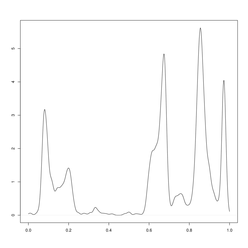
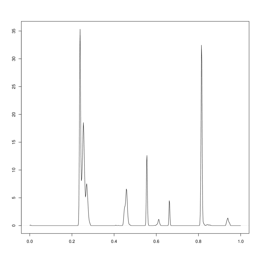
Figure 1. Simulated realizations of the density of the kernel $K_{0,1}(0,\cdot)$ associated with generators ${\mathcal{G}}^{N,1}$. The parameters are $a=20,b=0.375$ in (a), and $a=60,b=0.125$ in (b).

As $n$ tends to infinity these flows of kernels converge to the flow of kernels associated to a consistent family of sticky Brownian motions. Flows of this type were first considered by Le Jan and Raimond [lejan4]. For a general splitting rule, they were defined by Howitt and Warren [hw1], and have subsequently been studied extensively in [sss]. In general the parameters of a consistent family of sticky Brownian motions can represented in terms of a splitting measure $\nu$ as

(32) $$\theta(k:l)=\int_{0}^{1}q^{k-1}(1-q)^{l-1}\nu(dq)$$

For the parameters $\theta(k:l)$ given by Theorem 1, the measure $\nu$ is given by

(33) $$\nu(dq)=\frac{q(1-q)}{\phi(\Phi^{-1}(q))}dq$$

where $\phi$ denotes the standard Gaussian density, and $\Phi$ the corresponding distribution function. The right and left speeds of the flow are defined by

(34) $$\beta_{+}=2\int_{0}^{1}q^{-1}\nu(dq)\text{ and }\beta_{-}=-2\int_{0}^{1}(1-q)^{-1}\nu(dq)$$

and with $\nu$ given by (33) are both infinite. Thus according to the Theorem 2.7 of [sss], the support of the corresponding kernels is almost surely equal to ${\mathbf{R}}$. However, by Theorem 2.8 of [sss], for any $s\leq t$ and $x$ the measure $K_{s,t}(x,\cdot)$ is purely atomic. This seems consistent with the simulations which show the mass becomeing more concentrated as the parameters $a$ and $b$ increase and decrease respectively. It is less evident from these simulations that, in the limit, the set of points carrying the mass is dense.

Acknowledgements. This work was started during a visit to Université Paris-Sud, and I would like to thanks the mathematics department there, and Yves Le Jan in particular, for their hospitality. I’d also less to thank Peter Windridge for his help with writing the R code for the simulations.