Pumping single-file colloids: Absence of current reversal

Abstract

We consider the single-file motion of colloidal particles interacting via short-ranged repulsion and placed in a traveling wave potential, that varies periodically in time and space. Under suitable driving conditions, a directed time-averaged flow of colloids is generated. We obtain analytic results for the model using a perturbative approach to solve the Fokker-Planck equations. The predictions show good agreement with numerical simulations. We find peaks in the time-averaged directed current as a function of driving frequency, wavelength and particle density and discuss possible experimental realizations. Surprisingly, unlike a closely related exclusion dynamics on a lattice, the directed current in the present model does not show current reversal with density. A linear response formula relating current response to equilibrium correlations is also proposed.

In single-file motion, colloidal particles are confined to move in a narrow channel such that they cannot overtake each other. This was first studied by Hodgkin and Keynes hodgkin1955 while trying to describe ion transport in biological channels. One of the most interesting features of single-file motion is the sub-diffusive behavior that individual particles exhibit, and has been extensively studied both theoretically rodenbeck1998 ; lizana2008 ; barkai2009 ; roy2013 and experimentally Hahn1996 ; Kukla1996 ; Wei2000 ; Lutz2004 ; lin2005 ; das2010 . An exciting question has been that of obtaining directed particle currents in such single-file systems in closed geometries, for example colloidal particles moving in a circular micro-channel. Using periodic forces that vanish on the average, it has been possible to drive particle currents in a unidirectional manner. These are referred to as Brownian ratchets and may, for example, be achieved through continual switching on and off of a spatially asymmetric potential profile Julicher1997 ; Reimann2002 . Such phenomena have been studied experimentally using suitably constructed electrical gating Rousselet1994 ; Leibler1994 ; Marquet2002 , and with the help of laser tweezers Faucheux1995 ; Faucheux1995a ; Lopez2008 . Intracellular motor proteins like kinesin, myosin that move on respective filamentous tracks Reimann2002 , or ${\rm Na}^{+}$-, ${\rm K}^{+}$-ATPase pumps associated with the cell-membranes Gadsby2009 , are examples of naturally occurring stochastic pumps. With a few exceptions Derenyi1995 ; Derenyi1996 ; Aghababaie1999 ; Slanina2008a ; Slanina2009 ; savel2004 , most theoretical studies of Brownian ratchets focused on systems of non-interacting particles.

Recently a model of classical stochastic pump Chaudhuri2011 ; Marathe2008 ; Jain2007 has been proposed, similar to those used in the study of quantum pumps Brouwer1998 ; Citro2003 . Unlike Brownian ratchets, in these pump models, the colloidal particles are driven by a traveling wave potential. Thus, while typical ratchet models consider particles in a potential of the form $V(x,t)=f(x)g(t)$, the pump model considers a form such as $V(x,t)=V_{0}\cos(qx-\omega t)$. In Ref. Chaudhuri2011 , the dynamics of colloidal particles with short ranged repulsive interactions, and confined to move on a ring in the presence of an external space-time varying potential, was studied by considering a discretized version. In the discrete space model, particles moved on a lattice with the exclusion constraint that sites cannot have more than one particle and hopping rates between neighboring sites depended on the instantaneous potentials on the sites. This roughly mimics the over-damped Langevin dynamics of hard-core particles that is expected to be followed by sterically stabilized colloids. As expected, the traveling wave potential resulted in a DC particle current in the ring. An intriguing result was that the system showed a current direction-reversal on increasing the density beyond half-filling. This behavior was an outcome of the particle-hole symmetry of the discrete model Chaudhuri2011 . Current reversal has been observed in subsequent theoretical studies Dierl2014 ; pradhan14 . Further interesting properties of this model, including a detailed phase diagram, were recently obtained for the case where the system was connected to reservoirs and a biasing field applied Dierl2014 . General conditions for pumping to occur have recently been discussed in Rahav2008 ; Mandal2011 ; Asban2014 .

An important question is as to how much of the interesting qualitative features, seen in the lattice model, remain valid for real interacting colloidal particles executing single-file Brownian dynamics. This is one of the main motivations of this Letter. Here we consider the effect of a traveling wave potential on such particles which can be described by Langevin dynamics.

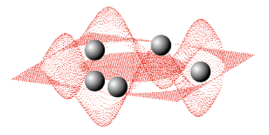
Figure 1: (Color online) A circular potential trap, which confines the motion of colloids in one dimension, is denoted by the white annulus. The colloidal particles are shown by dark spheres. The oscillatory profile indicates a time-frozen version of the traveling wave potential $V=V_{0}\cos(\omega t-qx)$.

Numerical and some analytic results based on the solution of the Fokker-Planck equation are presented. We derive a linear response formula for the DC current in terms of equilibrium correlation functions. We find that, unlike the lattice version Chaudhuri2011 ; Marathe2008 ; Jain2007 , there is no current-reversal in this system. A proposal for possible experimental realization of particle pumping in colloidal systems, using traveling waves, is discussed.

We consider $N$ colloidal particles that are confined to move on a one-dimensional ring of length $L$. The particles interact via potentials $U(x)$ that are sufficiently short ranged that we take them to be only between nearest neighbors. In addition, a weak traveling wave potential of the form $V(x,t)=\lambda k_{B}T\cos(\omega t-qx)$ with $\lambda<1$, acts on each particle. Let $x_{i}$, $i=1,2,\ldots,N$ denote the positions of the particles along the channel. Then the over-damped Langevin equations of motion of the system are given by

$$\frac{dx_{i}}{dt} =-\mu\frac{\partial\cal U}{\partial x_{i}}+\eta_{i},$$ (1)

$${\rm where}~{}{\cal U} =\sum_{i=1}^{N}V(x_{i})+\sum_{i=1}^{N}U(|x_{i}-x_{i+1}|)$$

is the total potential energy of the system and $\eta_{i}(t)$ is white Gaussian noise with $\langle\eta_{i}\rangle=0$, $\langle\eta_{i}(t)\eta_{j}(t^{\prime})\rangle=2D\delta_{i,j}\delta(t-t^{\prime}),~{}D=\mu k_{B}T$ is the diffusion constant, $\mu$ the mobility, $k_{B}$ the Boltzmann constant and $T$ the ambient temperature. We have taken periodic boundary conditions $x_{N+1}=L+x_{1}$.

Denoting the joint probability distribution of the $N$-particle system as $P({\bf x},t)$ with ${\bf x}=(x_{1},x_{2},\dots,x_{N})$, the Fokker-Planck equation governing its time evolution is

$$\partial_{t}P=\sum_{i}\partial_{x_{i}}[D\partial_{x_{i}}P+\mu P\partial_{x_{i}}{\cal U}]~{}.$$ (2)

The one-point distribution for the $i^{\rm th}$ particle is given by $P^{(1)}_{i}(x_{i},t)=\int dx_{1}dx_{2}\dots dx_{i-1}dx_{i+1}\ldots dx_{N}P({\bf x},t)$. Similarly let $P^{(2)}_{i,i+1}(x_{i},x_{i+1})$ be the two-point distribution obtained from $P({\bf x})$ by integrating out all coordinates other than $x_{i},x_{i+1}$. Let us then define the averaged distributions $P^{(1)}(x,t)=\frac{1}{N}\sum_{i}P^{(1)}_{i}(x,t)$ and $P^{(2)}(x,x^{\prime},t)=\frac{1}{N}\sum_{i}P^{(2)}_{i,i+1}(x,x^{\prime},t)$. Integrating the $N$-particle Fokker-Planck equation one finds a BBGKY hierarchy of equations, the first of which is

$$\partial_{t}P^{(1)}(x,t)= -\partial_{x}J~{},$$ (3)

$${\rm where}\,J= -D\partial_{x}P^{(1)}(x,t)-\mu\partial_{x}VP^{(1)}(x,t)$$

$$-\mu\int dx^{\prime}\partial_{x}U(|x-x^{\prime}|)P^{(2)}(x,x^{\prime},t).$$

The local density of particles is given by $\rho(x,t)=NP^{(1)}(x,t)$, and the corresponding current density is $j(x,t)=NJ(x,t)$. The time and space averaged directed current in the system is given by

$$j_{\rm DC}=\frac{1}{\tau L}\int_{0}^{\tau}dt\int_{0}^{L}dxj(x,t)~{},$$ (4)

where $\tau=2\pi/\omega$.

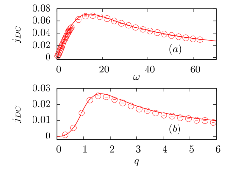
Figure 2: (Color online) Directed current $j_{\rm DC}$ as a function of ($a$) driving frequency $\omega$ and ($b$) driving wave-number $q$ in the non-interacting system. The points denote Langevin dynamics simulation results of free particles and the solid lines are the analytic prediction of Eq. (9). The parameters used are: number of particles $N=128$, mean density $\rho_{0}=0.3$, potential strength $\lambda=0.5$, diffusion constant $D=1$ and temperature $k_{B}T=1$. In (a) $q=1.2\,\pi$ while in (b) $\omega=\pi/2$.

Non-interacting system: We first analyze the non-interacting system ($U=0$). The Fokker-Planck equation for $\rho(x,t)$ is

$$\partial_{t}\rho(x,t)+\partial_{x}j=0,~{}~{}j(x,t)=-D\left[\beta V^{\prime}+\partial_{x}\right]\rho(x,t)~{}$$ (5)

with $V^{\prime}=\partial_{x}V$. We expand the density in a perturbative series in small parameter $\lambda$ as

$$\rho(x,t)=\rho_{0}+\sum_{k=1,2,\dots}\lambda^{k}\rho^{(k)}(x,t),$$ (6)

where $\rho_{0}=N/L$ is the mean density of particles. The mean directed current $j_{\rm DC}$ gets a contribution only from the drift part of the current in Eq. (5), which to leading order is given by $-D\beta V^{\prime}\lambda\rho^{(1)}$. The time evolution for $\rho^{(1)}$ is given by

$$\partial_{t}\rho^{(1)}-D\partial_{x}^{2}\rho^{(1)} = \rho_{0}D\partial_{x}^{2}(\beta V/\lambda)~{},$$ (7)

and this has the time-periodic steady state solution

$$\rho^{(1)} = \rho_{0}q^{2}D~{}{\rm Re}\left[\frac{e^{i(qx-\omega t)}}{i\omega-Dq^{2}}\right]~{}.$$ (8)

Thus, to leading order in the perturbation series in $\lambda$, the time averaged directed current is

$$j_{\rm DC} = \frac{1}{\tau L}\int_{0}^{\tau}dt\int_{0}^{L}dx(-\beta D\lambda\rho^{(1)}\partial_{x}V)$$ (9)

$$= \frac{\lambda^{2}\rho_{0}}{2}\frac{D^{2}q^{3}\omega}{D^{2}q^{4}+\omega^{2}}.$$

As expected, the current has a linear dependence on particle density $\rho_{0}$. The dependence on driving frequency $\omega$ and wave-number $q$ are plotted in Fig. (2) where we also show a comparison of the results from the analytic perturbative theory with those from direct numerical simulations for $\lambda=0.5$. We see that there is excellent agreement even for this, not very small, value of $\lambda$.

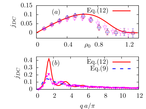
Figure 3: (Color online) Directed current $j_{\rm DC}$ as a function of ($a$) mean density $\rho_{0}$, and ($b$) wave number $q$ in the interacting system. The points denote Langevin dynamics simulation results of particles interacting via WCA ($\circ$), soft-core ($\triangle$), and Fermi-function step potentials ($\triangledown$). The solid lines in ($a$) and ($b$) are plots of Eq. (12) with $a=0.75$. Parameters are: $\omega=14$, and $\lambda=0.5$; in ($a$) $q=1.2\pi$, in ($b$) $\rho_{0}=0.55$.

Interacting system: Let us consider a hard-core interaction between the particles defined through the potential $U(x)=\infty$ if $|x|<a$ and $0$ otherwise. Since $NP^{(1)}=\rho(x,t)$ gives the density of particles and defining the pair distribution function $g(x,x^{\prime},t)$ through the relation $NP^{(2)}=\rho(x,t)g(x,x^{\prime},t)$, we see that Eq. (3) can equivalently be written as

$$\partial_{t} \rho(x,t)=D\partial^{2}_{x}\rho+\mu\partial_{x}\left[V(x,t)\rho(x,t)\right]$$

$$+\mu\partial_{x}\left[\rho(x,t)\int dx^{\prime}\partial_{x}U(|x-x^{\prime}|)g(x,x^{\prime},t)\right]~{}.$$ (10)

On expanding $\rho(x,t)$ and $g(x,x^{\prime},t)$ as perturbation series in $\lambda$ we find that the resulting equations do not close at successive orders. This is different from the case of the discrete systems studied in Chaudhuri2011 ; Marathe2008 ; Jain2007 where the perturbative solution works even in the presence of interactions. We thus need to make further approximations before applying the perturbation theory. It turns out that a mean-field description of the interaction term in Eq. (10) makes the problem tractable. The pair correlation function $g(x,x^{\prime},t)$ gives the probability of finding a particle at $x^{\prime}$ given that there is a particle at $x$, while $-\partial_{x}U(|x-x^{\prime}|)$ is the force on the particle at $x$ due to a particle at $x^{\prime}$. Hence the integral ${\cal I}=\int dx^{\prime}[-\partial_{x}U(|x-x^{\prime}|)]g(x,x^{\prime},t)$ has the interpretation of being the average force on a particle located at $x$. Next we note that for a hard rod centered at $x$, the force is localized at the points $x\pm a$, hence we can approximate the average force by the pressure difference between these points, i.e., ${\cal I}=\Pi(x-a)-\Pi(x+a)$. Here we assume that $\Pi(x,t)$ is the instantaneous local equilibrium pressure, finally we relate this pressure to the density $\rho(x,t)$ through the equilibrium relation $\Pi=k_{B}T\rho/[1-\rho a]$ Chowdhury2000 . Using this form of the interaction term and expanding $\rho(x,t)$ to first order in $\lambda$, the time evolution equation for $\rho^{(1)}$ is

$$\partial_{t}\rho^{(1)} -D\partial_{x}^{2}\rho^{(1)}=\rho_{0}D\partial_{x}^{2}(\beta V/\lambda)$$

$$+D\alpha\partial_{x}\left[\rho^{(1)}(x+a,t)-\rho^{(1)}(x-a,t)\right]~{},$$

where $\alpha=\rho_{0}/(1-\rho_{0}a)^{2}$. The time-periodic steady state solution of this equation is given by

$$\rho^{(1)}=\rho_{0}q^{2}D~{}{\rm Re}\left[\frac{e^{i(qx-\omega t)}}{i\omega-Dq^{2}-2D\alpha q\sin(qa)}\right]~{}.$$ (11)

This leads to, up to order $\lambda^{2}$ in perturbation series, the following average current

$$j_{\rm DC}=\frac{\lambda^{2}\rho_{0}}{2}\frac{D^{2}q^{3}\omega}{D^{2}[q^{2}+2\alpha q\sin(qa)]^{2}+\omega^{2}}~{}.$$ (12)

This is the first main result of our paper. We now see a non-trivial dependence on particle density $\rho_{0}$ and wave-number $q$. For a fixed density there is enhancement of particle current at some $q$ values [see Fig. (3)]. The current vanishes at the full-packing density $\rho_{0}=1/a$, as expected. However, unlike the lattice model, there is now no current reversal. In the discrete lattice model of symmetric exclusion process driven by a potential $\lambda\cos(\omega t-\phi n)$ with $n$ a lattice site and $\phi=qa$ Chaudhuri2011 ,

$$j_{\rm DC} = \lambda^{2}f_{0}^{2}(q_{0}-2k_{0})\frac{\omega\sin\phi(1-\cos\phi)}{\omega^{2}+4f_{0}^{2}(1-\cos\phi)^{2}},$$ (13)

where $f_{0}=D/a^{2}$, and $(q_{0}-2k_{0})=\eta(1-\eta)(1-2\eta)$ in the large $L/a$ limit with $\eta=\rho_{0}a$ the packing fraction. The dynamics had particle-hole symmetry leading to current reversal at $\eta=1/2$. In the continuum dynamics performed by colloidal particles, there is no such particle- hole symmetry. Note that the continuum limit of Eq.(13) with $a/L\to 0$, $\phi=qa\ll 1$ and $\eta=\rho_{0}a\ll 1$ leads to the result for non-interacting colloids Eq. (9). Presumably, the correct discrete model that one needs to consider, in order to get the correct continuum limit, is one where particles occupy a finite number (large) of sites and then one has to take appropriate limts.

Langevin dynamics simulations: To test our analytic predictions, we performed Langevin dynamics simulations of the model using Euler integration of Eq. (1). The time scale is set by $\tau_{D}=a^{2}/D$. For the non-interacting system, we used an integration time-step $\delta t=10^{-2}\tau_{D}$. For the interacting single-file case, in order to avoid unphysical particle crossings at large densities, we used $\delta t=10^{-5}\tau_{D}$. A total of $N=128$ particles were simulated. The particle flux is averaged over the system, and over a time period $100\tau$ where $\tau=2\pi/\omega$. The particle current is further averaged over $100$ realizations. The fluctuations over realizations provide the errors in the measured currents. To check the robustness of our results, we considered a number of smooth potentials to model the short-ranged inter-particle repulsion: (a) Weeks-Chandler-Anderson (WCA) potential Weeks1971 $\beta U(x)=4[(\sigma/x)^{12}-(\sigma/x)^{6}+1/4]$ if $|x|<2^{1/6}\sigma$ else $U=0$, (b) Soft core potential $\beta U(x)=(\sigma/x)^{12}-2^{-12}$ if $|x|<2\sigma$ else $U=0$, and (c) Fermi-function step potential $\beta U(x)=A/[\exp((x-a)/w)+1]$ with $A=100$, $w=0.02\sigma$ and $a=0.75\sigma$. In the simulations $k_{B}T=1/\beta$ and $\sigma$ set the energy and length scales respectively. The simulation data for all the three potentials agree with each other within numerical errors (Fig. 3($a$)). They show a non-monotonic variation with density, with maximal current near $\rho_{0}\sigma=0.55$. A plot of Eq. (12) with $a=0.75\sigma$ shows qualitative agreement with numerical data. Fig.3($b$) shows $j_{\rm DC}$ as a function of driving wave-number $q$ in a system of particles interacting via Fermi-function step potential. Multiple maxima in $j_{\rm DC}$ appears, in qualitative agreement with Eq. (12). A comparison with Eq. (9) shows another intriguing feature, directed current in presence of repulsive interaction can be higher than that of free particles.

Linear response theory: Even though the current response is ${\cal O}(\lambda^{2})$ and hence nonlinear in the perturbation, we note that it was obtained from the first order change in the density and hence should be calculable from linear response theory. We now show that it is indeed possible to express the current response to the perturbing traveling wave potential, in terms of equilibrium correlation functions of various forces, using linear response theory. Let us write the equation of motion in the form $\dot{x}_{i}=\mu[F_{i}(t)+f_{i}]+\eta_{i}$, where $F_{i}(t)=-\partial_{x_{i}}V(x_{i},t)$ and $f_{i}=-\partial_{x_{i}}U(|x_{i}-x_{i+1}|)-\partial_{x_{i}}U(|x_{i}-x_{i-1}|)$ is the total force on $i^{\rm th}$ particle from its neighbors. We see that the total current is given by $\int_{0}^{L}dx\langle j(x)\rangle=\sum_{i=1}^{N}\langle\dot{x}_{i}\rangle=\mu\sum_{i=1}^{N}\langle F_{i}\rangle$, where $\langle F_{i}\rangle=\int d{\bf x}F_{i}(x_{i},t)P({\bf x},t)$ . The long time solution $P({\bf x},t)$ can be obtained from perturbation theory. The Fokker-Planck equation for $P$, given by Eq. (2), can be expressed as $\partial_{t}P={\cal L}_{0}P+{\cal L}_{1}P$ where ${\cal L}_{0}=\sum_{i}[D\partial_{x_{i}}^{2}-\mu\partial_{x_{i}}f_{i}]$ and the external perturbation is ${\cal L}_{1}=-\sum_{i}\mu\partial_{x_{i}}F_{i}$. Writing $P=P_{0}+P_{1}$, where $P_{0}=\exp[-\beta\sum_{i}U(x_{i},x_{i+1})]/Z$ is the equilibrium state, one gets to $\cal O(\lambda)$, $P_{1}({\bf x},t)=\int_{-\infty}^{t}dt^{\prime}e^{{\cal L}_{0}(t-t^{\prime})}{\cal L}_{1}P_{0}({\bf x})$ . Using this, to leading order in $\lambda$, one obtains

$$\langle F_{i}\rangle=-\mu\int_{-\infty}^{t}dt^{\prime}\int d{\bf x}F_{i}(t)e^{{\cal L}_{0}(t-t^{\prime})}\sum_{j}\partial_{x_{j}}[F_{j}(t^{\prime})P_{0}({\bf x})]$$

$$=-\mu\int_{0}^{\infty}du\big{\langle}F_{i}(t)e^{{\cal L}_{0}u}\sum_{j}\left[\partial_{x_{j}}F_{j}(t-u)+\beta F_{j}(t-u)f_{j}\right]\big{\rangle}_{0},$$

where $\langle\ldots\rangle_{0}$ refers to an equilibrium average, and the time-dependence in $F_{i}(t)=F_{i}(x_{i},t)$ only refers to the explicit time-dependence of the external force. Using the fact that $F_{i}=-\lambda k_{B}Tq\sin(qx_{i}-\omega t)$ and that $\langle A(t)B(0)\rangle=\int d{\bf x}A({\bf x})e^{{\cal L}_{0}t}B({\bf x})P_{0}$ we get

$$\langle F_{i}\rangle=-\lambda^{2}q^{2}\mu(k_{B}T)^{2}\int_{0}^{\infty}du\big{\langle}\sin(qx_{i}(u)-\omega t)$$

$$\times\sum_{j}\left[q\cos(qx_{j}-\omega(t-u))+\beta f_{j}\sin(qx_{j}-\omega(t-u))\right]\big{\rangle}_{0}~{}.$$

Finally, after averaging over a time period we get for the DC current:

$$j_{DC} =\sum_{i,j}\frac{-(\lambda q\mu k_{B}T)^{2}}{2L}\int_{0}^{\infty}dt\Big{[}q\big{\langle}\sin[q(x_{i}(t)-x_{j})-\omega t]\big{\rangle}_{0}$$

$$+\big{\langle}\beta f_{j}\cos[q(x_{i}(t)-x_{j})-\omega t]\big{\rangle}_{0}\Big{]}~{}.$$ (14)

This linear response formula, relating the DC current to equilibrium correlation functions, is the second main result of this paper.

Possible experiment: Using oscillating mirrors, it is possible to move a strongly focused infrared laser beam along a circle to constrain $\sigma\approx 1\mu$m sized polystyrene spheres to move along a circle Faucheux1995 . The steric interaction between polystyrene beads would lead to single-file motion. Using similar techniques as in Faucheux1995 , one can generate a cosine potential by passing the laser through an appropriately graded filter. Finally, a traveling wave potential can be formed by rotating the filter at the required frequency. If we choose the driving force wavelength to be few particle sizes so that $qa\approx 1$ then the optimal driving frequency is $\omega\approx Dq^{2}\approx D/a^{2}\approx 1Hz$, using $D\approx 1\mu{\rm m}^{2}{\rm s}^{-1}$ at room temperature. This leads to a current $j_{\rm DC}\approx 0.05{\rm s}^{-1}$ at a density $\rho_{0}a\approx 0.5$. This is comparable to the currents obtained using the flashing ratchet mechanism in Faucheux1995 .

In summary, we investigated the dynamics of interacting colloidal particles confined to move in a narrow circular channel and driven by a traveling wave potential. Using a combination of mean-field type assumptions and perturbation theory, analytic results were obtained for the average particle current in the channel. This compares quite well with simulation results. We have also proposed a linear response formula relating the current response to equilibrium correlations. This relation opens up further analytic possibilities. The current shows peaks as a function of driving frequency and wave number, and also the particle density. The current vanishes as we approach the close packing limit and, rather surprisingly, does not show current reversal unlike what is seen in studies of discrete versions of this model Chaudhuri2011 . From the point of view of experiments, the pumping of colloidal particles in narrow channels using traveling wave potentials looks very accessible and could have potential applications.

- (1) A. L. Hodgkin and R. Keynes, The Journal of Physiology 128, 61 (1955).
- (2) C. Rödenbeck, J. Kärger, and K. Hahn, Physical Review E 57, 4382 (1998).
- (3) L. Lizana and T. Ambjörnsson, Physical Review Letters 100, 200601 (2008).
- (4) E. Barkai and R. Silbey, Physical Review Letters 102, 050602 (2009).
- (5) A. Roy, O. Narayan, A. Dhar, and S. Sabhapandit, Journal of Statistical Physics 150, 851 (2013).
- (6) K. Hahn, J. Kärger, and V. Kukla, Phys. Rev. Lett. 76, 2762 (1996).
- (7) V. Kukla, J. Kornatowski, D. Demuth, I. Girnus, H. Pfeifer, L. V. C. Rees, S. Schunk, K. K. Unger, and J. Karger, Science 272, 702 (1996).
- (8) Q. Wei, C. Bechinger, and P. Leiderer, Science 287, 625 (2000).
- (9) C. Lutz, M. Kollmann, P. Leiderer, and C. Bechinger, J. Phys. Cond. Matt. 16, S4075 (2004).
- (10) B. Lin, M. Meron, B. Cui, S. A. Rice, and H. Diamant, Physical Review Letters 94, 216001 (2005).
- (11) A. Das, S. Jayanthi, H. S. M. V. Deepak, K. V. Ramanathan, A. Kumar, C. Dasgupta, and A. K. Sood, ACS nano 4, 1687 (2010).
- (12) F. Jülicher, A. Ajdari, and J. Prost, Reviews of Modern Physics 69, 1269 (1997).
- (13) P. Reimann, Physics Reports 361, 57 (2002).
- (14) J. Rousselet, L. Salome, A. Ajdari, and J. Prost, Nature 370, 446 (1994).
- (15) S. Leibler, Nature 370, 412 (1994).
- (16) C. Marquet, A. Buguin, L. Talini, and P. Silberzan, Physical Review Letters 88, 168301 (2002).
- (17) L. Faucheux, L. Bourdieu, P. Kaplan, and A. Libchaber, Physical Review Letters 74, 1504 (1995).
- (18) L. P. Faucheux, G. Stolovitzky, and A. Libchaber, Phys. Rev. E 51, 5239 (1995).
- (19) B. Lopez, N. Kuwada, E. Craig, B. Long, and H. Linke, Physical Review Letters 101, 220601 (2008).
- (20) D. C. Gadsby, A. Takeuchi, P. Artigas, and N. Reyes, Philosophical transactions of the Royal Society of London. Series B, Biological sciences 364, 229 (2009).
- (21) I. Derényi and T. Vicsek, Physical Review Letters 75, 374 (1995).
- (22) I. Derenyi and A. Ajdari, Physical Review E 54, R5 (1996).
- (23) Y. Aghababaie, G. Menon, and M. Plischke, Physical Review E 59, 2578 (1999).
- (24) F. Slanina, EPL (Europhysics Letters) 84, 50009 (2008).
- (25) F. Slanina, Physical Review E 80, 061135 (2009).
- (26) S. Savel’ev, F. Marchesoni, and F. Nori, Phys. Rev. E 70, 061107 (2004).
- (27) D. Chaudhuri and A. Dhar, EPL (Europhysics Letters) 94, 30006 (2011).
- (28) R. Marathe, K. Jain, and A. Dhar, Journal of Statistical Mechanics: Theory and Experiment 2008, P11014 (2008).
- (29) K. Jain, R. Marathe, A. Chaudhuri, and A. Dhar, Physical Review Letters 99, 190601 (2007).
- (30) P. Brouwer, Physical Review B 58, R10135 (1998).
- (31) R. Citro, N. Andrei, and Q. Niu, Physical Review B 68, 165312 (2003).
- (32) M. Dierl, W. Dieterich, M. Einax, and P. Maass, Physical Review Letters 112, 150601 (2014).
- (33) R. Chatterjee, S. Chatterjee, P. Pradhan, and S. S. Manna, Phys. Rev. E 89, 022138 (2014).
- (34) S. Rahav, J. Horowitz, and C. Jarzynski, Physical Review Letters 101, 140602 (2008).
- (35) D. Mandal and C. Jarzynski, Journal of Statistical Mechanics: Theory and Experiment 2011, P10006 (2011).
- (36) S. Asban and S. Rahav, Physical Review Letters 112, 050601 (2014).
- (37) D. Chowdhury and D. Stauffer, Principles of Equilibrium Statistical Mechanics (Wiley-VCH, Weinheim, 2000).
- (38) J. D. Weeks, The Journal of Chemical Physics 54, 5237 (1971).