Time-stepping discontinuous Galerkin methods for fractional diffusion problems

Abstract

Time-stepping $hp$-versions discontinuous Galerkin (DG) methods for the numerical solution of fractional subdiffusion problems of order $-\alpha$ with $-1<\alpha<0$ will be proposed and analyzed. Generic $hp$-version error estimates are derived after proving the stability of the approximate solution. For $h$-version DG approximations on appropriate graded meshes near $t=0$, we prove that the error is of order $O(k^{\max\{2,p\}+\frac{\alpha}{2}})$, where $k$ is the maximum time-step size and $p\geq 1$ is the uniform degree of the DG solution. For $hp$-version DG approximations, by employing geometrically refined time-steps and linearly increasing approximation orders, exponential rates of convergence in the number of temporal degrees of freedom are shown. Finally, some numerical tests are given.

1 Introduction

In this work, time-stepping discontinuous Galerkin methods (DGMs) for fractional order diffusion equations of the form

$$u^{\prime}+{\mathcal{B}}_{\alpha}Au=f\qquad~{}{\rm on}~{}~{}\Omega\times(0,T]\quad{\rm with}~{}~{}u|_{t=0}=u_{0},$$ (1)

subject to homogeneous Dirichlet boundary conditions are proposed and analyzed, where $u=u(x,t)$, $f=f(x,t)$, $u_{0}=u_{0}(x)$ ($(x,t)\in\Omega\times(0,T]$), $u^{\prime}=\frac{\partial u}{\partial t}$, and

$${\mathcal{B}}_{\alpha}v(t)=\frac{\partial}{\partial t}\int_{0}^{t}\omega_{\alpha+1}(t-s)\,v(s)\,ds~{}~{}{\rm with}~{}~{}{\omega_{\alpha+1}}(t)=\frac{t^{\alpha}}{\Gamma(\alpha+1)}$$ (2)

is the Riemann–Liouville time fractional derivative operator of order $0<-\alpha<1$.

In (1), the spatial domain $\Omega$ is assumed to be bounded and polyhedral, and for simplicity, we choose $Au=-{\rm div}(K_{\alpha+1}\nabla u)$ with $\nabla$ being the spatial gradient of $u$ and $K_{\alpha+1}>0$ (positive constant) is the diffusivity. Thus, $A$ (subject to homogeneous Dirichlet boundary conditions) is strictly positive-definite and possesses a complete orthonormal eigensystem $\{\phi_{m}\}_{m=1}^{\infty}$ in $L_{2}(\Omega)$. We let $\lambda_{m}$ denote the eigenvalue corresponding to $\phi_{m}$ (i.e., $A\phi_{m}=\lambda_{m}\phi_{m}$ with $\phi_{m}|_{\partial\Omega}=0$) where (without loss of generality) we assume for convenience that $0<\lambda_{1}\leq\lambda_{2}\leq\lambda_{3}\leq\cdots$.

Problems of the form (1) arise in a variety of physical, biological and chemical applications KilbasSrivastavaTrujillo2006 ; Mathai2011 ; SokolovKlafter2005 ; Tarasov2011 . It describes anomalous subdiffusion and occurs, for example, in models of fractured or porous media, where the particle flux depends on the entire history of the density gradient $\nabla u$.

A variety of low-order numerical methods for problems of the form (1) (with Riemann–Liouville or Grünwald–Letnikov fractional derivatives) were studied by several authors. For explicit, implicit Euler and compact finite difference (FD) schemes, see for example ChenLiuTurnerAnh2010 ; Cui2009 ; LanglandsHenry2005 ; LiuYangBurrage2009 ; Mustapha2011 ; YusteAcedo2005 ; YusteQuintana2009 ; ZhuangLiuAnhTurner2008 ; ZhuangLiuAnhTurner2009 . For ADI FD schemes on a rectangular spatial domain; refer to WangWang2011 ; ZhangSun2011 . In addition, various numerical methods Cui2012 ; Cui2013 ; GaoSun2011 ; JinLazarovZhou2012 ; MustaphaAbdallahFurati2014 ; Quintana-MurilloYuste2011 ; SweilamKhaderMahdy2012 ; ZhangSun2011 have also been applied for the following alternative representation of (1) (using the Caputo derivatives): $I^{-\alpha}u^{\prime}(t)-{\rm div}(K_{\alpha+1}\nabla u)(t)=\tilde{f}(t)$ where $I^{-\alpha}$ is the Riemann–Liouville time fractional integral operator;

$$I^{-\alpha}v(t):=\int_{0}^{t}\omega_{-\alpha}(t-s)v(s)\,ds\quad{\rm for}~{}~{}-1<\alpha<0\,.$$

The two representations are equivalent under suitable assumptions on the initial data, but the methods obtained for each representation are formally different.

In earlier papers, McLean and I proposed and analyzed different low-order time stepping DG schemes for problem (1). In McLeanMustapha2009 , a piecewise-constant DGM (generalized backward Euler) combined with finite elements (FEs) for the spatial discretization was studied. Unconditional stability and optimal convergence rates in both time and space were proved. Using a different approach, we later studied MustaphaMcLean2012IMA the error analysis of the piecewise-linear DGM. Suboptimal rates of convergence had been achieved, however, the numerical results illustrated optimal rates. In continuation, by duality arguments, nodal superconvergence results were proved in MustaphaMcLean2012SINUM . Moreover, we extracted the superconvergence at the nodal points of the DG solution globally by post-processing the DG solution through Lagrange interpolations. In all these papers, variable time steps were employed to compensate the lack of regularity of the solution $u$ of problem (1) near $t=0$.

The main purpose of this paper is to study the stability and the accuracy of high-order time-stepping $h$-version DG ($h$-DG) and $hp$-version ($hp$-DG) methods. This task is not trivial since the DGM allows us to only control the jumps of the approximate solutions which is enough for the low-order DGMs in McLeanMustapha2009 ; MustaphaMcLean2011 ; MustaphaMcLean2012IMA ; MustaphaMcLean2012SINUM . A new analysis based on the coercivity and continuity properties of the operator ${\mathcal{B}}_{\alpha}$, also based on some fractional derivative-integral identities is required. These will be the keys to establish the stability and consequently deriving promising error estimates (in the $L_{\infty}(0,T)$-norm) over families of nonuniform meshes.

In contrast, for $0<\alpha<1,$ the model problem (1) amounts to the fractional wave equation (super-diffusion):

$$u^{\prime}(t)+I^{\alpha}Au(t)=f(t)\quad{\rm with}~{}~{}u|_{t=0}=u_{0}\,.$$ (3)

Recently, Schötzau and I investigated MustaphaSchoetzau2013 $h$-DG and $hp$-DG methods (in time) for problem (3). Although we could not show the stability of our scheme because of some technical difficulties, algebraic and exponential convergence rates (in a non-standard norm that can be weaker than the $L_{2}$-norm in some cases) for $h$-DG and $hp$-DG schemes were achieved, respectively.

Due to the different nature and properties of the operators $I^{\alpha}$ and ${\mathcal{B}}_{\alpha}$, another technique will be used in this work to show the stability of our scheme and also to derive generic $hp$-version abstract error estimates in the stronger $L_{\infty}(0,T)$-norm. Then proceeding along the lines of MustaphaBrunnerMustaphaSchoetzau2011 ; MustaphaSchoetzau2013 ; SchoetzauSchwab00 and investigating two refinement strategies in the case where the solution $u$ of (1) lacks regularity as $t=0$. Noting that, in MustaphaBrunnerMustaphaSchoetzau2011 ; SchoetzauSchwab00 , $hp$-DGMs for parabolic and parabolic integro-differential equations were considered where the stability and error analyses follow relatively straight forwardly from the different natures of the equations.

In the $L_{\infty}(0,T)$-norm, exponential convergence rates (in the number of temporal degrees of freedom) for the $hp$-version DG ($hp$-DG) scheme based on geometrically refined time-steps and on linearly increasing approximation orders will be achieved. Moreover, for the $h$-DGM of piecewise uniform degree $p\geq 1$, we prove $O(k^{\max\{2,p+\frac{1}{2}\}+\frac{\alpha}{2}})$ algebraic convergence rates over non-uniform graded meshes that concentrate the time levels near $t=0$. So, the convergence rates is short $\frac{1-\alpha}{2}$ power from being optimal for $p\geq 2$, however, just short by $-\frac{\alpha}{2}$ power for $p=1$ which is due to the fact that the approximate solution can be controlled from the jumps in this case. Indeed, the numerical experiments illustrate optimal error rates of order $O(k^{p+1})$ for some choices of $\alpha$ and $p$. In our test we combine the proposed $hp$-version time-stepping method with a standard (continuous) FEs in space which will then define a fully discrete scheme. We choose the spatial step size and the order of the spatial FEs so that the temporal errors are dominating. Analyzing the convergence of the fully discrete scheme will be considered in future work.

Motivation of the $hp$-DG and future work. The nonlocal nature of ${\mathcal{B}}_{\alpha}$ means that on each time subinterval, one must efficiently evaluate a sum of integrals over all previous time subintervals. For example, a direct implementation of the time-stepping $h$-DG method (of uniform degree $p$) combined with the FE discretization in space requires $\mathcal{O}((p+1)\,N^{2}\,M)$ operations and requires $\mathcal{O}((p+1)\,N\,M)$ storage ($N$ is the number of time-mesh elements and $M$ is the spatial degrees of freedom). Thus, reducing the number of time-steps and at the same time maintaining high accuracy is important especially when $\Omega\subset{\mathbb{R}}^{3}$, then the time-space problem (1) is four-dimensional and thus beyond the computing power of conventional machines. For analytic solutions in the time variable, $hp$-DGMs with exponential rates of convergence allow us to achieve these requirements to a large extent. For instance, if the error from the spatial FE is of order $\mathcal{O}(h^{r})$ for some $r\geq 2,$ then we can balance the exponential rates in time with the algebraic one in space. In this case, the number of operations will be reduced to $\mathcal{O}((p+1)\,M\,(\log M)^{\nu_{2}})$ and the active operations to $\mathcal{O}((p+1)\,M(\log M)^{\nu_{2}})$ where $\nu_{1}$ and $\nu_{2}$ depend on $r$. However, if the solution $u$ of (1) is not analytic (in time) but satisfies appropriate regularity assumptions, time-space sparse grids can be used to get similar results. Furthermore, if in addition $u$ satisfies certain mixed spatial regularity properties, the computational cost can be further reduced. These computing issues are subject to ongoing investigation and hence, will be considered in future work.

The outline of the paper is as follows. The DGM will be introduced in the next section and the stability of the semi-discrete solutions will be proved in Section 3. Followed by deriving abstract error bounds of the time-stepping DGM in Section 4. Sections 5 and 6 are devoted to establishing algebraic rate of convergence of the $h$-DGM and exponential rates of convergence for the $hp$-DGM, respectively. Numerical illustrations of our results will be presented in Section 7.

2 Discontinuous Galerkin discretization

To define the time-stepping DGM for problem (1), we introduce a partition ${\cal M}$ of the interval $[0,T]$ given by the points: $0=t_{0}<t_{1}<\cdots<t_{N}=T.$ We set $I_{n}=(t_{n-1},t_{n})$ and $k_{n}=t_{n}-t_{n-1}$ for $1\leq n\leq N$. With each subinterval $I_{n}$ we associate a polynomial degree $p_{n}\in{\mathbb{N}}_{0}$. These degrees are then stored in the degree vector ${\bf p}:=(p_{1},p_{2},\cdots,p_{N}).$ Next, we introduce the discontinuous finite element space

$${\mathcal{W}}({\cal M},{\bf p})=\left\{\,v:[0,T]\to H^{1}_{0}(\Omega)\,:\,v|_{I_{n}}\in\mathbb{P}_{p_{n}},\ 1\leq n\leq N\right\},$$ (4)

where $\mathbb{P}_{p_{n}}$ denotes the space of polynomials of degree $\leq p_{n}$ with coefficients in $H^{1}_{0}(\Omega)$. For a function $v\in{\mathcal{W}}({\cal M},{\bf p})$, we write $v^{n}_{-}=v(t_{n}^{-})$, $v_{+}^{n}=v(t_{n}^{+})$ and $[v]^{n}=v^{n}_{+}-v^{n}_{-}$ with $v^{N}_{+}=v^{N}_{-}$ and $v_{-}^{0}=v^{0}\,.$

The time-stepping DG approximation $U\in{\mathcal{W}}({\cal M},{\bf p})$ is now defined as follows: Given $U(t)$ for $t\in\cup_{j=1}^{n-1}I_{j-1}$, the discrete solution $U\in\mathbb{P}_{p_{n}}$ on the next time subinterval  $I_{n}$ is determined by requesting that

$$\langle U^{n-1}_{+}-U^{n-1}_{-},X^{n-1}_{+}\rangle+\int_{t_{n-1}}^{t_{n}}\,\Big{(}\langle U^{\prime},X\rangle+A({\mathcal{B}}_{\alpha}U,X)\,\Big{)}\,dt=\int_{t_{n-1}}^{t_{n}}\langle f,X\rangle\,dt$$ (5)

$\forall~{}X\in\mathbb{P}_{p_{n}}$ with  $U^{0}_{-}\approx u_{0}$. Here $A(\cdot,\cdot):H^{1}_{0}(\Omega)\times H^{1}_{0}(\Omega)\to\mathbb{R}$ is bilinear operator associated with the differential operator $A:=-{\rm div}(K_{\alpha+1}\nabla)$ and is given by

$$A(v,w):=\langle\nabla v,\nabla w\rangle=\sum_{m=1}^{\infty}\lambda_{m}\,u_{m}\,v_{m}\quad\text{where $u_{m}=\langle u,\phi_{m}\rangle$ and $v_{m}=\langle v,\phi_{m}\rangle$}\,.$$

Throughout the paper, by $\langle\cdot,\cdot\rangle$ and $\|\cdot\|$, we denote the inner product and the associated norm in the space $L_{2}(\Omega)$. Moreover, $\|\cdot\|_{1}$ denotes the norm on the Sobolev space $H^{1}(\Omega)$ and for $j\geq 1$, $u^{(j)}:=\frac{\partial^{j}u}{\partial t^{j}}$.

As in MustaphaSchoetzau2013 , since the operator $A$ possesses a complete orthonormal eigensystem $\{\lambda_{m},\phi_{m}\}_{m\geq 1}$, the DG scheme  (5) can be reduced to a finite linear system of algebraic equations on each subinterval $I_{n}$. To see this, let $P_{p_{n}}$ be the scalar polynomial space of degree $\leq p_{n}$. Now, take $X=\phi_{m}w$ in (5), we find that: for $m\geq 1,$

$$U_{m,+}^{n-1}\;w^{n-1}_{+}+\int_{t_{n-1}}^{t_{n}}\,\Bigl{(}{U^{\prime}_{m}}w+\lambda_{m}{\mathcal{B}}_{\alpha}U_{m}\;w\,\Bigr{)}\,dt\\ =U^{n-1}_{m,-}\;w^{n-1}_{+}+\int_{t_{n-1}}^{t_{n}}f_{m}\,w\,dt$$ (6)

$\forall~{}w\in P_{p_{n}}$ and for $1\leq n\leq N,$ where $U_{m}=\langle U,\phi_{m}\rangle\in P_{p_{n}}$ and $f_{m}=\langle f,\phi_{m}\rangle$.

Very briefly, because of the finite dimensionality of system (6), the existence of the scalar function $U_{m}$ on $I_{n}$ follows from its uniqueness. For uniqueness, it is enough to show that $U_{m}\equiv 0$ on $I_{n}$ for $n\geq 1$ when the right-hand side of (6) is identically zero. This follows from the stability theorem (Theorem 3.1) and the coercivity property (i) in Lemma 1.

3 Stability of DG solutions

In this section, we show the stability of the semi-discrete solutions. For convenience, we introduce the following notation. Set $J:=\bigcup_{j=1}^{N}I_{j}$ and we let ${\mathcal{C}}^{1}(J)$ denote the space of functions $v:J\to\mathbb{R}$ such that the restriction $v|_{I_{j}}$ extends to a continuously differentiable function on the closed interval $[t_{j-1},t_{j}]$, for $1\leq j\leq N$.

In the following result we gather two key properties of the fractional time derivative operator ${\mathcal{B}}_{\alpha}$ that we use in our analysis.

Lemma 1

Let $c_{\alpha}=\frac{\cos(\alpha\pi/2)}{\pi^{\alpha}}\frac{|\alpha|^{-\alpha}}{(1-\alpha)^{1-\alpha}}$ and $d_{\alpha}=\frac{1}{\cos(\alpha\pi/2)}$ for any $-1<\alpha<0$. Then, for any $v,\,w$ in ${\mathcal{C}}^{1}(J)$ (or in $W^{1,1}(0,T)$), we have

• $\int_{0}^{T}{\mathcal{B}}_{\alpha}v(t)\,v(t)\,dt\geq c_{\alpha}T^{\alpha}\int_{0}^{T}v^{2}(t)\,dt,$

• $\Big{|}\int_{0}^{T}{\mathcal{B}}_{\alpha}v(t)\,w(t)\,dt\Big{|}^{2}\leq{d_{\alpha}}^{2}\int_{0}^{T}{\mathcal{B}}_{\alpha}v(t)\,v(t)\,dt\int_{0}^{T}{\mathcal{B}}_{\alpha}w(t)\,w(t)\,dt\,.$

Proof

The coercivity property (i) was proven in (McLean2012, , Theorem A.1) by using the Laplace transform and the Plancherel Theorem. In a similar fashion, property (ii) can be obtained, see for example (MustaphaSchoetzau2013, , Lemma 3.1).$\quad\Box$

Remark 1

Noting that, as $\alpha$ approaches $0$, we recover the classical coercivity and continuity properties. In addition, as was mentioned earlier, for $0<\alpha<1,$ ${\mathcal{B}}_{\alpha}=I^{\alpha}$. In this case, the above coercivity property is no longer valid. We have a weaker version instead, see (MustaphaSchoetzau2013, , Lemma 3.1 (i)). $\quad\Box$

The stability of the DG solution $U$ will be shown in the next theorem. The proof below looks straightforward due to the new approach that has not been used before. The key ingredients are the above lemma and the appropriate use of the identity: ${\mathcal{B}}_{\alpha}I^{-\alpha}=I.$ Indeed, the current approach can be adopted to show the stability of $U$ when $0<\alpha<1$ as this was not proven in MustaphaSchoetzau2013 . It is worth mentioning that the stability result below plays a crucial role in our forthcoming error analysis, see Theorem 4.2. Noting that, the proofs of the stability in McLeanMustapha2009 ; MustaphaMcLean2011 are valid only for $h$-DGMs of order $p\in\{0,1\}$ (low-order).

Theorem 3.1

For $1\leq n\leq N$, the DG solution $U$ of (5) satisfies

$$\|U_{-}^{n}\|^{2}+\|U^{n-1}_{+}\|^{2}+2\,\int_{0}^{t_{n}}\,A({\mathcal{B}}_{\alpha}U,U)\,dt\leq 4\,\|U_{-}^{0}\|^{2}+4\,d_{\alpha}^{2}\int_{0}^{t_{n}}|\langle g,A^{-1}f\rangle|\,dt$$

where $A^{-1}$ is the inverse of the positive-definite operator $A$, and $g(t):=(I^{-\alpha}f)(t)\,.$

Proof

Choosing $X=U$ in (5) and using $\langle U^{\prime}(t),U(t)\rangle=\frac{1}{2}\frac{d}{dt}\|U(t)\|^{2}$, we obtain

$$\|U_{-}^{j}\|^{2}+\|U^{j-1}_{+}\|^{2}-2\langle U_{-}^{j-1},U^{j-1}_{+}\rangle+2\int_{t_{j-1}}^{t_{j}}\,A({\mathcal{B}}_{\alpha}U,U)\,dt=2\int_{t_{j-1}}^{t_{j}}\langle f,U\rangle\,dt.$$

Summing over $j=1,\cdots,\ell$, and using $f={\mathcal{B}}_{\alpha}g,$

$$\sum_{j=1}^{\ell}\bigl{(}\|U_{-}^{j}\|^{2}+\|U^{j-1}_{+}\|^{2}-2\langle U_{-}^{j-1},U^{j-1}_{+}\rangle\bigr{)}+2\int_{0}^{t_{\ell}}\,A({\mathcal{B}}_{\alpha}U,U)\,dt\\ =2\,\int_{0}^{t_{\ell}}\langle{\mathcal{B}}_{\alpha}g,U\rangle\,dt.$$

Choose $\ell=n-1$ and $\ell=n$ respectively, summing and then using the identity;

$$\sum_{j=1}^{\ell}\bigl{(}\|U_{-}^{j}\|^{2}+\|U^{j-1}_{+}\|^{2}-2\langle U_{-}^{j-1},U^{j-1}_{+}\rangle\bigr{)}\\ =\|U_{-}^{\ell}\|^{2}+\|U^{0}_{+}\|^{2}+\sum_{j=1}^{\ell-1}\|[U]^{j}\|^{2}-2\langle U_{-}^{0},U^{0}_{+}\rangle$$

yield

$$\|U_{-}^{n-1}\|^{2}+\|U_{-}^{n}\|^{2}+2\|U^{0}_{+}\|^{2}+\|[U]^{n-1}\|^{2}+2\sum_{j=n-1}^{n}\int_{0}^{t_{j}}\,A({\mathcal{B}}_{\alpha}U,U)\,dt\\ \leq 4\langle U_{-}^{0},U^{0}_{+}\rangle+2\sum_{j=n-1}^{n}\int_{0}^{t_{j}}\langle{\mathcal{B}}_{\alpha}g,U\rangle\,dt.$$

Since $4|\langle U_{-}^{0},U^{0}_{+}\rangle|\leq 2\|U_{-}^{0}\|^{2}+2\|U^{0}_{+}\|^{2}$ and $\|U^{n-1}_{+}\|^{2}\leq 2\|U_{-}^{n-1}\|^{2}+2\|[U]^{n-1}\|^{2}$,

$$\|U_{-}^{n}\|^{2}+\|U^{n-1}_{+}\|^{2}+4\sum_{j=n-1}^{n}\int_{0}^{t_{j}}\,A({\mathcal{B}}_{\alpha}U,U)\,dt\\ \leq 4\,\|U_{-}^{0}\|^{2}+4\sum_{j=n-1}^{n}\int_{0}^{t_{j}}\langle{\mathcal{B}}_{\alpha}g,U\rangle\,dt,$$ (7)

for $1\leq n\leq N$. Now, setting $U_{m}=\langle U,\phi_{m}\rangle$ and $g_{m}=\langle g,\phi_{m}\rangle$, and hence, the continuity property (ii) in Lemma 1 implies that; for $1\leq j\leq N$,

$$4\,\int_{0}^{t_{j}}\langle{\mathcal{B}}_{\alpha}g,U\rangle\,dt =4\sum_{m=1}^{\infty}\,\int_{0}^{t_{j}}{\mathcal{B}}_{\alpha}g_{m}\,U_{m}\,dt$$

$$\leq 4\,d_{\alpha}\sum_{m=1}^{\infty}\,\left(\int_{0}^{t_{j}}{\mathcal{B}}_{\alpha}g_{m}\,g_{m}\,dt\right)^{1/2}\left(\int_{0}^{t_{j}}{\mathcal{B}}_{\alpha}U_{m}\,U_{m}\,dt\right)^{1/2}\,dt$$

$$\leq 2\,d_{\alpha}^{2}\sum_{m=1}^{\infty}\,\int_{0}^{t_{j}}{\mathcal{B}}_{\alpha}g_{m}\,\lambda_{m}^{-1}g_{m}\,dt+2\sum_{m=1}^{\infty}\lambda_{m}\int_{0}^{t_{j}}{\mathcal{B}}_{\alpha}U_{m}\,U_{m}\,dt$$

$$=2\,d_{\alpha}^{2}\int_{0}^{t_{j}}\langle{\mathcal{B}}_{\alpha}g,A^{-1}g\rangle\,dt+2\,\int_{0}^{t_{j}}A({\mathcal{B}}_{\alpha}U,U)\,dt\,.$$

Therefore, the desired stability estimate follows after inserting the above bound (for $j=n-1$ and $j=n$) on the right-hand side of (7) . This finishes the proof.$\quad\Box$

4 Error analysis

This section is devoted to deriving abstract error estimates for the DGM. A global formulation of our numerical scheme will be given first. More precisely, it will be convenient to reformulate the DG scheme (5) in terms of the bilinear form

$$G_{N}(U,X)=\langle U^{0}_{+},X^{0}_{+}\rangle+\sum_{n=1}^{N-1}\langle[U]^{n},X^{n}_{+}\rangle+\int_{0}^{t_{N}}\,\Bigl{(}\langle U^{\prime},X\rangle+A({\mathcal{B}}_{\alpha}U,X)\Bigr{)}\,dt.$$ (8)

Integration by parts yields an alternative expression for the bilinear form $G_{N}$:

$$G_{N}(U,X)=\langle U^{N}_{-},X^{N}_{-}\rangle-\sum_{n=1}^{N-1}\langle U^{n}_{-},[X]^{n}\rangle+\int_{0}^{t_{N}}\,\Bigl{(}-\langle U,X^{\prime}\rangle+A({\mathcal{B}}_{\alpha}U,X)\Bigr{)}\,dt.$$ (9)

By summing up (5) over all time-steps, the DGM can now equivalently be written as: Find $U\in{\mathcal{W}}({\cal M},{\bf p})$ such that

$$G_{N}(U,X)=\langle U^{0}_{-},X^{0}_{+}\rangle+\int_{0}^{t_{N}}\langle f,X\rangle\,dt\qquad\forall\,X\in{\mathcal{W}}({\cal M},{\bf p}).$$ (10)

Let $u$ be the solution of (1) and $U$ the DG approximation defined in (10). Decomposing the error $U-u$ into the two terms:

$$U-u=(U-\Pi u)+(\Pi u-u)=:\theta+\eta\,.$$ (11)

where $\Pi u\in{\mathcal{W}}({\cal M},{\bf p})$ is the $hp$-version projection of $u$ defined by: for $1\leq n\leq N,$

$$\Pi u(t_{n}^{-})-u(t_{n})=0\quad\text{and}\quad\int_{t_{n-1}}^{t_{n}}\,\langle u\,-\Pi u,v\rangle\,dt=0\quad\forall\,v\in\mathbb{P}_{p_{n}-1},$$ (12)

The bound of $\eta$ follows from the next theorem.

Theorem 4.1

Let $1\leq n\leq N$ and $0\leq q_{n}\leq p_{n}$. If $u^{(q_{n}+1)}|_{I_{n}}\in L_{2}(I_{n};H^{1}(\Omega))$, then

$$\int_{t_{n-1}}^{t_{n}}\|(\Pi u-u)^{\prime}\|^{2}_{1}\,dt\leq C\,p_{n}^{2}\left(\frac{k_{n}}{2}\right)^{2q_{n}}\Gamma_{p_{n},q_{n}}\int_{t_{n-1}}^{t_{n}}\|u^{(q_{n}+1)}\|^{2}_{1}\,dt$$

where $\Gamma_{p_{n},q_{n}}=\frac{\Gamma(p_{n}-q_{n}+1)}{\Gamma(p_{n}+q_{n}+1)}$ and the constant $C$ is independent of $k_{n}$, $p_{n}$, $q_{n}$, and $u$.

Proof

See  (SchoetzauSchwab00, , Section 3) for the proof.$\quad\Box$

The main task now is to estimate  $\theta$. To do so, we use the contribution from the stability results, the continuity property of the operator ${\mathcal{B}}_{\alpha}$, the inverse inequality, in addition to some other technical steps. In comparison to the case $0<\alpha<1$, the achieved bound of $\theta$ in MustaphaSchoetzau2013 is weaker (by far) than the one below. This is due to the different properties of ${\mathcal{B}}_{\alpha}$ and ${\mathcal{I}}^{\alpha}$ and also because of the technique used here.

Theorem 4.2

Assume that the time-step sizes are nondecreasing. Then, for $1\leq n\leq N,$ if the solution $u\in W^{1,1}((0,t_{n});H^{1}_{0}(\Omega))$, we have

$$|\theta|_{n}^{2}+\frac{k_{n}^{\min\{1,p_{n}-1\}}}{p_{n}^{2}}\Big{(}\sup_{t\in I_{n}}\|\theta(t)\|^{2}\Big{)}\\ \leq C_{\alpha,T}\left(\,\|U^{0}_{-}-u_{0}\|^{2}+t_{n}\max_{j=1}^{n}k_{j}^{\alpha}\,\big{(}\int_{t_{j-1}}^{t_{j}}\|\eta^{\prime}\|_{1}dt\big{)}^{2}\right),$$

where $|\theta|_{n}:=\max\{\|\theta^{n-1}_{+}\|,\|\theta^{n}_{-}\|\}$.

Proof

Since $G_{n}(u,X)=\langle u_{0},X^{0}_{+}\rangle+\int_{0}^{t_{n}}\langle f,X\rangle\,dt$, we have

$$G_{n}(U-u,X)=\langle U^{0}_{-}-u_{0},X^{0}_{+}\rangle\qquad\forall\,X\in{\mathcal{W}}({\cal M},{\bf p}).$$

Hence, the alternative expression for $G_{N}$ in (9), and the fact that $\eta^{n}=0$ and $\int_{t_{n-1}}^{t_{n}}\langle\eta,X^{\prime}\rangle\,dt=0$ for all $1\leq n\leq N$, by definition of the operator $\Pi$ (note that for $p_{n}=0$, we have $X^{\prime}\equiv 0$), yield

$$G_{n}(\theta,X) =\langle U_{-}^{0}-u_{0},X^{0}_{+}\rangle-G_{n}(\eta,X)=\langle U_{-}^{0}-u_{0},X^{0}_{+}\rangle+\int_{0}^{t_{n}}\,A({\mathcal{B}}_{\alpha}\eta,X)\,dt$$

for all $X\in{\mathcal{W}}({\cal M},{\bf p})$. Since this equation has the same form as (10), following the proof of the stability in Theorem 3.1, we notice that for $1\leq n\leq N$,

$$|\theta|_{n}^{2}+2\,\int_{0}^{t_{n}}A({\mathcal{B}}_{\alpha}\theta,\theta)\,dt\leq 4\,\|U^{0}_{-}-u_{0}\|^{2}+4\,d_{\alpha}^{2}\,\max_{j=n-1}^{n}\int_{0}^{t_{j}}A({\mathcal{B}}_{\alpha}\eta,\eta)\,dt\,.$$ (13)

To estimate the last term, we use the equality $\eta(t)=-\int_{t}^{t_{j}}\eta^{\prime}(q)\,dq$ for $t\in I_{j}$, then changing the order of integrations and integrating,

$$\int_{0}^{t_{n}}A({\mathcal{B}}_{\alpha}\eta,\eta)\,dt =-\sum_{j=1}^{n}\int_{t_{j-1}}^{t_{j}}\int_{t}^{t_{j}}A({\mathcal{B}}_{\alpha}\eta(t),\eta^{\prime}(q))\,dq\,dt$$ (14)

$$=-\sum_{j=1}^{n}\int_{t_{j-1}}^{t_{j}}\int_{t_{j-1}}^{q}A({\mathcal{B}}_{\alpha}\eta(t),\eta^{\prime}(q))\,dt\,dq$$

$$=\sum_{j=1}^{n}\int_{t_{j-1}}^{t_{j}}A({\mathcal{I}}^{-\alpha}\eta(t_{j-1})-{\mathcal{I}}^{-\alpha}\eta(q),\eta^{\prime}(q))\,dq$$

$$=\sum_{j=1}^{n}{\mathcal{I}}_{1}^{j}+\sum_{j=1}^{n}{\mathcal{I}}_{2}^{j}$$

where

$$\begin{split}{\mathcal{I}}_{1}^{j}&:=-\int_{t_{j-1}}^{t_{j}}\int_{t_{j-1}}^{q}\omega_{\alpha+1}(q-s)A(\eta(s),\eta^{\prime}(q))\,ds\,dq\\ &=\int_{t_{j-1}}^{t_{j}}\int_{t_{j-1}}^{q}\int_{s}^{t_{j}}\omega_{\alpha+1}(q-s)A(\eta^{\prime}(t),\eta^{\prime}(q))\,dt\,ds\,dq\end{split}$$

and

$$\begin{split}{\mathcal{I}}_{2}^{j}&:=\int_{t_{j-1}}^{t_{j}}\int_{0}^{t_{j-1}}[\omega_{\alpha+1}(t_{j-1}-s)-\omega_{\alpha+1}(q-s)]A(\eta(s),\eta^{\prime}(q))\,ds\,dq\\ &=-\sum_{i=1}^{j-1}\int_{t_{j-1}}^{t_{j}}\int_{t_{i-1}}^{t_{i}}\int_{s}^{t_{i}}[\omega_{\alpha+1}(t_{j-1}-s)-\omega_{\alpha+1}(q-s)]A(\eta^{\prime}(t),\eta^{\prime}(q))\,dt\,ds\,dq\,.\end{split}$$

To bound ${\mathcal{I}}_{1}^{j}$ and ${\mathcal{I}}_{2}^{j}$, we use the Cauchy-Schwarz inequality and integrating

$${\mathcal{I}}_{1}^{j} \leq\int_{t_{j-1}}^{t_{j}}\|\nabla\eta^{\prime}(t)\|\int_{t_{j-1}}^{q}\omega_{\alpha+1}(q-s)\int_{t_{j-1}}^{t_{j}}\|\nabla\eta^{\prime}(q)\|\,dt\,ds\,dq$$

$$\leq\omega_{2+\alpha}(k_{j})\Big{(}\int_{t_{j-1}}^{t_{j}}\|\eta^{\prime}\|_{1}dt\Big{)}^{2}$$

and

$${\mathcal{I}}_{2}^{j} \leq\sum_{i=1}^{j-1}\int_{t_{j-1}}^{t_{j}}\|\nabla\eta^{\prime}(q)\|\int_{t_{i-1}}^{t_{i}}[\omega_{\alpha+1}(t_{j-1}-s)-\omega_{\alpha+1}(t_{j}-s)]\int_{s}^{t_{i}}\|\nabla\eta^{\prime}(t)\|\,dt\,ds\,dq$$

$$\leq\max_{i=1}^{j}\,\left(\int_{t_{i-1}}^{t_{i}}\|\nabla\eta^{\prime}\|dt\right)^{2}\,\int_{0}^{t_{j-1}}[\omega_{\alpha+1}(t_{j-1}-s)-\omega_{\alpha+1}(t_{j}-s)]\,ds$$

$$\leq\omega_{2+\alpha}(k_{j})\max_{i=1}^{j}\Big{(}\int_{t_{i-1}}^{t_{i}}\|\eta^{\prime}\|_{1}dt\Big{)}^{2}\,.$$

Now, inserting the estimates of ${\mathcal{I}}_{1}^{j}$ and ${\mathcal{I}}_{2}^{j}$ in (14), and using the mesh assumption $k_{i}\leq k_{j}$ for $i\leq j$. This implies

$$\int_{0}^{t_{n}}A({\mathcal{B}}_{\alpha}\eta,\eta)\,dt\leq\frac{2\,t_{n}}{\Gamma(\alpha+2)}\max_{j=1}^{n}k_{j}^{\alpha}\,\Big{(}\int_{t_{j-1}}^{t_{j}}\|\eta^{\prime}\|_{1}dt\Big{)}^{2},$$

and therefore, for $1\leq n\leq N$,

$$|\theta|_{n}^{2}+2\,\int_{0}^{t_{n}}A({\mathcal{B}}_{\alpha}\theta,\theta)\,dt\leq 4\,\|U^{0}_{-}-u_{0}\|^{2}+\frac{4\,t_{n}\,d_{\alpha}^{2}}{\Gamma(\alpha+2)}\max_{j=1}^{n}k_{j}^{\alpha}\Big{(}\int_{t_{j-1}}^{t_{j}}\|\eta^{\prime}\|_{1}dt\Big{)}^{2}\,.$$

But, for $p_{n}=1$, the left-hand side is $\geq\sup_{t\in I_{n}}\|\theta(t)\|^{2}$, however for $p_{n}\geq 2$, it is

$$\geq c_{\alpha}\,t_{n}^{\alpha}\int_{t_{n-1}}^{t_{n}}\|\nabla\theta\|^{2}\,dt\geq C\,c_{\alpha}t_{n}^{\alpha}\int_{t_{n-1}}^{t_{n}}\|\theta\|^{2}\,dt\geq C\,c_{\alpha}t_{n}^{\alpha}\frac{k_{n}}{p_{n}^{2}}\Big{(}\sup_{t\in I_{n}}\|\theta(t)\|^{2}\Big{)}$$

by the assumption that the operator $A$ possesses a complete orthonormal eigensystem $\{\lambda_{m},\phi_{m}\}_{m=1}^{\infty}$, the coercivity property in Lemma 1 (i), and the Poincare’s ($\theta|_{\partial\Omega}=0$) and inverse ($\theta|_{I_{n}}\in\mathbb{P}_{p_{n}}$) inequalities. This completes the proof.$\quad\Box$

The main abstract error bound will be derived in the next theorem. For convenience, we introduce the following notation:

$$\|\phi\|_{L_{\infty}(L_{2})}:=\|\phi\|_{L_{\infty}((0,T);L_{2}(\Omega))}=\max_{n=1}^{N}\Big{(}\sup_{t\in I_{n}}\|\phi(t)\|\Big{)}.$$

Theorem 4.3

Let $u$ be the solution of (1) and $U$ be the DG solution defined by (5) with $U^{0}_{-}=u_{0}$ (for simplicity). Assume that $k_{i}\leq k_{j}$ for $i\leq j$. Then we have

$$\max_{n=1}^{N}\{\|U^{n-1}_{+}-u(t_{n-1})\|,\|U^{n}_{-}-u(t_{n})\|\}\\ +\min_{n=1}^{N}\left(t_{n}^{-1}k_{n}^{\min\{1,p_{n}-1\}}\right)\frac{\|u-U\|_{L_{\infty}(L_{2})}^{2}}{\max_{n=1}^{N}p_{n}^{2}}\leq C_{\alpha,T}\,\max_{n=1}^{N}k_{n}^{\alpha}\Big{(}\int_{t_{n-1}}^{t_{n}}\|\eta^{\prime}\|_{1}dt\Big{)}^{2}\,.$$

Proof

This bound follows from the decomposition of the error in (11), the triangle inequality, Theorem 4.2, and the fact (by the interpolation properties of the operator $\Pi$), $\|\eta\|_{L_{\infty}(L_{2})}=\max_{1\leq n\leq N}\Big{(}\sup_{t\in I_{n}}\|\eta(t)\|\Big{)}\leq\max_{1\leq n\leq N}\int_{t_{n-1}}^{t_{n}}\|\eta^{\prime}\|dt\,.$ $\quad\Box$

5 $h$-version errors

In this section, we focus on the explicit error bounds of the $h$-DG solution $U$ of uniform degree $p$ on each subinterval $I_{n}$ for $2\leq n\leq N.$ Because of the singular behavior of the solution $u$ of (1) near $t=0,$ the degree of $U$ on the first subinterval $I_{1}$ will be chosen to be one (i.e., $p_{1}=1$). So, ${\bf p}=(1,p,\cdots,p)$. However, the numerical results suggested that this modification is not always needed. More precisely, we are required to consider $p_{1}=1$ if the time mesh, (16), is strongly graded.

Following McLeanMustapha2009 ; MustaphaMcLean2011 ; MustaphaMcLean2012IMA , we assume that the solution $u$ of (1) satisfies:

$$\|u^{(j)}(t)\|_{1}\leq M\,t^{\sigma-j}\qquad\forall\,1\leq j\leq p+1,$$ (15)

for some positive constants $M$ and $\sigma$; for a proof we refer the reader to McLean2010 ; McLeanMustapha2007  .

To compensate for singular behaviour of $u$ near $t=0$, we employ a family of non-uniform meshes denoted by ${\cal M}_{\gamma}$, where the time-steps are graded towards $t=0$. Following McLeanMustapha2009 ; MustaphaMcLean2011 ; MustaphaMcLean2012IMA ; MustaphaMcLean2012SINUM , for a fixed parameter $\gamma\geq 1$, we assume that

$$t_{n}=(nk)^{\gamma}\quad{\rm with}~{}~{}k=\frac{T^{1/\gamma}}{N}\quad\text{for ~{}~{}$0\leq n\leq N$.}$$ (16)

Noting that the time step sizes are nondecreasing, that is, $k_{i}\leq k_{j}$ for $i\leq j$. Moreover, one can show that

$$k_{n}\leq\gamma kt_{n}^{1-1/\gamma}~{}~{}{\rm for}~{}~{}n\geq 1~{}~{}{\rm and}~{}~{}t_{n}\leq 2^{\gamma}t_{n-1}~{}{\rm for}~{}~{}n\geq 2\,.$$ (17)

In the next theorem, we derive the error estimate for the $h$-DG solution over the graded mesh $\cal M_{\gamma}$ . In the $L_{\infty}(0,T)$-norm, we prove an $O(k^{\max\{2,p+\frac{1}{2}\}+\frac{\alpha}{2}})$ convergence rate, i.e., short by $-\frac{\alpha}{2}$ power from being optimal for $p=1$ and by $\frac{1-\alpha}{2}$ power for $p\geq 2$. However, the numerical results indicate optimal $O(k^{p+1})$-rates for $p\geq 1$. Indeed, these results are high-order extensions (also improvements) of the ones shown in McLeanMustapha2009 ; MustaphaMcLean2011 ; MustaphaMcLean2012IMA for $p\in\{0,1\}.$ In contrast, for $0<\alpha<1$, we successfully proved optimal $O(k^{p+1})$ convergence rates in (MustaphaSchoetzau2013, , Theorem 4.9), but in a much weaker norm. Noting that, the proof here is more technical but the general approach is partially similar to the proof of Theorem 4.9 in MustaphaSchoetzau2013 .

Theorem 5.1

Let the solution $u$ of (1) satisfy the regularity property (15). Let $U\in{\mathcal{W}}({\cal M}_{\gamma},{\bf p})$ be the $h$-DG approximation with $U^{0}_{-}=u_{0}$. Then for $\gamma\geq 1$, we have

$$\|U-u\|_{L_{\infty}(L_{2})}\leq C\,\times\begin{cases}k^{\min\{\gamma(\sigma+\frac{\alpha}{2}),2+\frac{\alpha}{2}\}}&\quad{\rm for}\quad p=1,\\ k^{\min\{\gamma(\sigma+\frac{\alpha}{2}),p+1+\frac{\alpha}{2}\}-\frac{1}{2}}&\quad{\rm for}\quad p\geq 2\end{cases}$$

where $C$ is a constant that depends only on $T$, $\alpha$, $\gamma$, $\sigma$ and $p$.

Proof Theorem 4.3 yields

$$\min\{1,\min_{n=2}^{N}\big{(}t_{n}^{-1}k_{n}^{\min\{1,p-1\}}\big{)}\}\|u-U\|_{L_{\infty}(L_{2})}^{2}\\ \leq C\,k_{1}^{\alpha}\left(\int_{0}^{t_{1}}\|\eta^{\prime}\|_{1}\right)^{2}+C\max_{n=2}^{N}k_{n}^{\alpha+1}\int_{t_{n-1}}^{t_{n}}\|\eta^{\prime}\|_{1}^{2}.$$

Since

$$t_{n}^{-1}k_{n}^{\min\{1,p-1\}}=1-\frac{t_{n-1}}{t_{n}}=1-\left(1-1/n\right)^{\gamma}\geq 1/n\geq 1/N~{}{\rm for}~{}p\geq 2,$$

$$\frac{1}{N^{\min\{1,p-1\}}}\|u-U\|_{L_{\infty}(L_{2})}^{2}\leq C\,k_{1}^{\alpha}\left(\int_{0}^{t_{1}}\|\eta^{\prime}\|_{1}dt\right)^{2}+C\max_{n=2}^{N}k_{n}^{\alpha+1}\int_{t_{n-1}}^{t_{n}}\|\eta^{\prime}\|_{1}^{2}dt.$$

On the subinterval $I_{1}$, $\Pi u\in\mathbb{P}_{1}$ and satisfies:

$$\Pi u(t_{1}^{-})=u(t_{1})\quad\text{and}\quad\int_{0}^{t_{1}}\bigl{[}u(t)-\Pi u(t)]\,dt=0\,.$$

Explicitly, the derivative of the interpolation error admits the integral representations (MustaphaMcLean2009, , Equation (3.8)):

$$\eta^{\prime}(t) =-u^{\prime}(t)+\frac{2}{k_{1}^{2}}\int_{0}^{t_{1}}s\,u^{\prime}(s)\,ds,\quad\text{for $t\in I_{1}$.}$$ (18)

So, from the triangle inequality and (18), we notice that

$$\int_{0}^{t_{1}}\,\|\eta^{\prime}\|_{1}\,dt\leq\int_{0}^{t_{1}}\left(\|u^{\prime}(t)\|_{1}+\frac{2}{k_{1}}\,\int_{0}^{t_{1}}\|u^{\prime}(s)\|_{1}\,ds\right)\,dt\leq 3\int_{0}^{t_{1}}\|u^{\prime}(t)\|_{1}\,dt\,.$$

Thus, using the regularity assumption, (15), and the mesh property, (17),

$$k_{1}^{\alpha}\left(\int_{0}^{t_{1}}\|\eta^{\prime}\|_{1}dt\right)^{2}\leq C\,k_{1}^{\alpha}\Bigl{(}\int_{0}^{t_{1}}t^{\sigma-1}\,dt\Bigr{)}^{2}=C\frac{k_{1}^{2\sigma+\alpha}}{\sigma}\leq Ck^{\gamma(2\sigma+\alpha)}\quad{\rm for}~{}~{}\gamma\geq 1\,.$$ (19)

In addition, for $n\geq 2$, we use Theorem 4.1 and get

$$k_{n}^{\alpha+1}\int_{t_{n-1}}^{t_{n}}\|\eta^{\prime}\|_{1}^{2}dt \leq Ck_{n}^{2p+\alpha+1}\int_{t_{n-1}}^{t_{n}}\|u^{(p+1)}\|^{2}dt$$

$$\leq C\,k_{n}^{2p+2+\alpha}{t_{n}}^{2(\sigma-1-p)}$$

$$\leq C\,k^{2p+2+\alpha}t_{n}^{2\sigma+\alpha-(2p+2+\alpha)/\gamma}$$

$$\leq C\,k^{\min\{\gamma(2\sigma+\alpha),2p+2+\alpha\}}\quad{\rm for}~{}~{}\gamma\geq 1.\quad\Box$$

6 $hp$-version errors

We discuss the error results of the $hp$-DGM based on geometrically refined time-steps and linearly increasing approximation orders. Following MustaphaBrunnerMustaphaSchoetzau2011 ; MustaphaSchoetzau2013 , we consider the $hp$-DGM for problems with solutions that have start-up singularities as $t\to 0$, but are analytic for $t>0$. More precisely, we stipulate that the solution $u$ of (1) has the analytic regularity:

$$\|u^{(j)}(t)\|+t\|u^{(j)}(t)\|_{1}\leq M\,d^{j}\Gamma(j+1)t^{\sigma-j}\qquad\forall\,t\in(0,T],\ \forall\,j\geq 1,$$ (20)

for positive constants $\sigma$, $M$ and $d$. Proving the regularity statement (20) remains an open issue, which is beyond the scope of the present paper.

To resolve the singular behavior of the solution near $t=0$, we shall make use of geometrically refined time-steps and linearly increasing degree vectors, and apply the $hp$-techniques that were developed in MustaphaBrunnerMustaphaSchoetzau2011 ; MustaphaSchoetzau2013 ; SchoetzauSchwab00 . To describe this, we first partition $(0,T)$ into (coarse) time intervals $\{\mathfrak{J}_{i}\}_{i=1}^{\bf K}$. The first interval $\mathfrak{J}_{1}=(0,T_{1})$ is then further subdivided geometrically into $L+1$ subintervals $\{I_{n}\}_{n=1}^{L+1}$ as follows:

$$t_{0}=0,\qquad t_{n}=\delta^{L+1-n}T_{1}\quad\text{for $1\leq n\leq L+1$}.$$ (21)

As usual, we call $\delta\in(0,1)$ the geometric refinement factor, and $L$ is the number of refinement levels. From (21), we observe that the subintervals $\{I_{n}\}_{n=1}^{L+1}$ satisfy

$$k_{n}=t_{n}-t_{n-1}=\lambda t_{n-1}\quad{\rm with}\quad\lambda=(1-\delta)/\delta\quad{\rm for}~{}~{}n\geq 2.$$ (22)

Let ${\cal M}_{L,\delta}$ be the mesh on $(0,T)$ defined in this way. The polynomial degree distribution $\bf p$ on ${\cal M}_{L,\delta}$ is defined as follows. On the first coarse interval $\mathfrak{J}_{1}$ the degrees are chosen to be linearly increasing:

$$p_{n}=\lfloor\mu n\rfloor\qquad\text{for $1\leq n\leq L+1$},$$ (23)

for a slope parameter $\mu>0$. On the coarse time intervals $\{\mathfrak{J}_{i}\}_{i=2}^{\bf K}$ away from $t=0$, we set the approximation degrees uniformly to $p_{L+1}=\lfloor\mu(L+1)\rfloor$. The resulting $hp$-version finite element space is denoted by ${\mathcal{W}}({\cal M}_{L,\delta},\bf p)$.

Our main result of this section suggests that non-smooth solutions satisfying (20) can be approximated at exponential rates convergence on the $hp$-version discretizations introduced above. This will be done by proceeding along the lines of (MustaphaBrunnerMustaphaSchoetzau2011, , Theorem 4.2) in our earlier work.

Theorem 6.1

Let $U\in{\mathcal{W}}({\cal M}_{L,\delta},{\bf p})$ be the $hp$-DG approximation with $U_{-}^{0}=u_{0}$. Then there exists a slope $\mu_{0}>0$ depending on $\delta$ and the constants $\sigma$ and $d$ in (20) such that for linearly increasing polynomial degree vectors ${\bf p}$ with slope $\mu\geq\mu_{0}$,

$$\|U-u\|_{L_{\infty}(L_{2})}\leq C\,{\rm exp}(-b\sqrt{{\mathcal{N}}}),$$

with positive constants $C$ and $b$ that are independent of  ${\mathcal{N}}:=\dim({\mathcal{W}}({\cal M}_{L,\delta},{\bf p}))$, but depending on the problem parameters $T$ and $\alpha$, the regularity parameters $M$, $d$ and $\sigma$ in (20), and the mesh parameters $\delta$, $T_{1}$ and $\mu$.

Proof

From the geometric mesh assumptions (21)–(22), we notice that $t_{i}^{-1}k_{i}=1-\delta$ for $1\leq i\leq L+1$. Hence, using Theorem 4.3 and obtain

$$\|U-u\|^{2}_{L_{\infty}(L_{2})}\leq Cp_{L+1}^{2}\max\{1/(1-\delta),{\bf K}\}(E_{1}+E_{2}),$$ (24)

where

$$\begin{split}E_{1}&=k_{1}^{\alpha}\left(\int_{I_{1}}\|\eta^{\prime}\|_{1}dt\right)^{2}+\max_{i=2}^{L+1}k_{i}^{\alpha+1}\int_{t_{i-1}}^{t_{i}}\|\eta^{\prime}\|_{1}^{2}dt\\ E_{2}&=\max_{i=2}^{K}(T_{i}-T_{i-1})^{\alpha+1}\,\int_{T_{i-1}}^{T_{i}}\|\eta^{\prime}\|_{1}^{2}dt\,.\end{split}$$

Since the solution $u$ is analytic on the coarse elements ${\mathfrak{J}}_{i}$, $2\leq i\leq{\bf K}$, from Theorem 4.1 and the approximation results for analytic functions in (Schwab98, , Theorem 3.19) yields an error estimate of the form

$$E_{2}\leq C_{1}\,{\rm exp}(-b_{1}L).$$ (25)

On the first subinterval $I_{1}$ adjacent to $t=0$, $\Pi u\in\mathbb{P}_{1}$. Hence, we follow the steps in (19), and then using the regularity assumption (20) and the geometric mesh properties, (21),

$$k_{1}^{\alpha}\left(\int_{0}^{t_{1}}\|\eta^{\prime}\|_{1}dt\right)^{2}\leq C\,k_{1}^{\alpha}\Bigl{(}\int_{0}^{t_{1}}t^{\sigma-1}\,dt\Bigr{)}^{2}=C\frac{k_{1}^{2\sigma+\alpha}}{\sigma}\leq C_{2}{\rm exp}(-b_{2}L).$$ (26)

On the subintervals $I_{j}$ for $2\leq j\leq L+1$, from the regularity property (20), we readily conclude that

$$\int_{t_{j-1}}^{t_{j}}\|u^{(q_{j}+1)}\|_{1}^{2}dt \leq C\,d^{2q_{j}}\Gamma(q_{j}+1)^{2}\int_{t_{j-1}}^{t_{j}}\,t^{2(\sigma-1-q_{j})}\,dt$$

$$\leq C\,k_{j}\,d^{2q_{j}}\Gamma(q_{j}+1)^{2}t_{j-1}^{2(\sigma-1-q_{j})},$$

and hence, we use Theorem 4.1 and the equality $k_{j}=\lambda\,t_{j-1}$ with $t_{j-1}\leq\delta^{L+2-j}T_{1}$ (from (22) and (21)), and get

$$\begin{split}k_{j}^{\alpha+1}\int_{t_{j-1}}^{t_{j}}\|\eta^{\prime}\|_{1}^{2}dt&\leq C\,\Gamma_{p_{j},q_{j}}\,p_{j}^{2}\left(\frac{k_{j}}{2}\right)^{2(q_{j}+1)+\alpha}d^{2q_{j}}\Gamma(q_{j}+1)^{2}t_{j-1}^{2(\sigma-1-q_{j})}\\ &\leq C\,\Gamma_{p_{j},q_{j}}\,p_{j}^{2}\,\left(\frac{d\lambda}{2}\right)^{2q_{j}}\Gamma(q_{j}+1)^{2}\delta^{(2\sigma+\alpha)(L+2-j)}\,.\end{split}$$

Using interpolation arguments analogous to (Schwab98, , Lemma 3.39), it can be seen that the above inequality also holds for any non-integer regularity parameter $q_{j}$ with $0\leq q_{j}\leq p_{j}$. Thus, we take $q_{j}=c_{j}p_{j}$ with $c_{j}\in(0,1)$ and proceed as in (Schwab98, , Theorem 3.36), and obtain

$$\Gamma_{p_{j},q_{j}}\,\left(\frac{d\lambda}{2}\right)^{2q_{j}}\Gamma(q_{j}+1)^{2}\leq Cp_{j}\left(\left(\frac{\lambda dc_{j}}{2}\right)^{2c_{j}}\frac{(1-c_{j})^{1-c_{j}}}{(1+c_{j})^{1+c_{j}}}\right)^{p_{j}}.$$

Noting that

$$\underset{0<c_{j}<1}{\inf}\left(\frac{\lambda\,dc_{j}}{2}\right)^{2c_{j}}\frac{(1-c_{j})^{1-c_{j}}}{(1+c_{j})^{1+c_{j}}}=:\ell_{\lambda,d}(c_{\min})<1\quad{\rm with}~{}~{}c_{\min}=\frac{1}{\sqrt{1+(\lambda d/2)^{2}}},$$

and consequently, choosing $c_{j}=c_{\min}$ and $p_{j}=\lfloor\mu j\rfloor\geq\mu_{0}j$ with $\mu_{0}>0$ such that $\left(\ell_{\lambda,d}(c_{\min})\right)^{\mu_{0}}=\delta^{(2\sigma+\alpha)},$ we conclude that

$$k_{j}^{\alpha+1}\int_{t_{j-1}}^{t_{j}}\|\eta^{\prime}\|_{1}^{2}dt \leq C\delta^{(2\sigma+\alpha)L}p_{L+1}^{3}\,(\ell_{\lambda,d}(c_{\min}))^{p_{j}}\delta^{-(2\sigma+\alpha)j}$$ (27)

$$\leq C\delta^{(2\sigma+\alpha)L}p_{L+1}^{3}\leq C_{3}{\rm exp}(-b_{3}L).$$

where we have absorbed the term $p_{L+1}^{3}$ into the constants $C_{3}$ and $b_{3}$.

Finally, by referring to (24), (25), (26) and (27) yields

$$\|U-u\|^{2}_{L_{\infty}(L_{2})}\leq C_{4}\,{\rm exp}(-b_{4}L),$$

where we have absorbed the term $p_{L+1}^{2}\max\{1/(1-\delta),{\bf K}\}$ in (24) into the constant $C_{4}$ and $b_{4}$. Finally, since ${\mathcal{N}}=\dim({\mathcal{W}}({\cal M}_{L,\delta},{\bf p}))\leq CL^{2}$ for $L$ sufficiently large, we obtain the desired result.$\quad\Box$

7 Numerical results

In this section, we demonstrate the validity of the achieved error estimates for both the h-DG and hp-DG time-stepping schemes, for problems of the form (1) when $Au=-u_{xx}$ and $\Omega=(0,1)$. To compute our numerical solution, we discretize in space using the standard FEs. So, we construct a family of uniform partitions of the domain $\Omega$ into subintervals with step size $h$, and let $S_{h}\subset H_{0}^{1}(\Omega)$ denote the space of continuous, piecewise polynomial functions of degree $\leq r$ with $r\geq 1$. The discontinuous finite element space (4) is now modified to the fully discrete finite dimensional space

$${\mathcal{W}}({\cal M},{\bf p},S_{h})=\left\{\,U_{h}:[0,T]\to S_{h}\,:\,U_{h}|_{I_{n}}\in\mathbb{P}_{p_{n}}(S_{h}),\ 1\leq n\leq N\,\right\}$$ (28)

where by $\mathbb{P}_{p}(S_{h})$ we denote the space of polynomials of degree $\leq p$ in the time variable with coefficients in $S_{h}$.

We define our fully-discrete time-stepping DG-spatial FE scheme as follows: find $U_{h}\in{\mathcal{W}}({\cal M},{\bf p},S_{h})$ such that

$$G_{N}(U_{h},X) =\langle R_{h}u_{0},X^{0}_{+}\rangle+\int_{0}^{t_{N}}\,\langle f(t),X(t)\rangle\,dt\qquad\forall\,X\in{\mathcal{W}}({\cal M},{\bf p},S_{h})$$ (29)

where $G_{N}$ is the global bilinear form defined as in (8) and $R_{h}:H_{0}^{1}(\Omega)\to S_{h}$ is the Ritz projection given by $A(R_{h}v,\chi)=A(v,\chi)$ for all $\chi\in S_{h}$ .

To demonstrate the validity of the algebraic and exponential convergence results of Theorems 5.1 and  6.1 for the fully discrete version scheme, we choose $h$ (the spatial step size) and $r$ (the degree of the approximate FE solution in the spatial variable) so that the temporal errors are dominating. To evaluate the errors, we introduce the finer grid

$${\mathcal{G}}^{m}=\{\,t_{j-1}+nk_{j}/m\,:\,1\leq j\leq N,\ 0\leq n\leq m\,\}$$ (30)

($N$ is the number of time mesh subintervals). Thus, for large values of $m$, the error measure $|||v|||_{m}:=\max_{t\in{\mathcal{G}}^{m}}\|v(t)\|$ approximate the norm $\|v\|_{L_{\infty}(L_{2})}$. To compute the spatial $L_{2}$-norm, we apply a composite Gauss quadrature rule with $(r+1)$ points on each interval of the finest spatial mesh.

Example: We choose the initial datum such that the exact solution is:

$$u(x,t)={\sin}(\pi x)-t^{\alpha+2}{\sin}(2\pi x).$$ (31)

$N$	$\gamma=1$		$\gamma=1.3$		$\gamma=1.6$
18	8.32e-04		2.78e-04		1.93e-04
27	4.80e-04	1.35	1.36e-04	1.76	8.28e-05	2.08			$p=1$
36	3.27e-04	1.34	8.28e-05	1.73	4.59e-05	2.05
72	1.31e-04	1.32	2.53e-05	1.71	1.12e-05	2.03
$N$	$\gamma=1$		$\gamma=1.6$		$\gamma=2.3$		$\gamma=3$
18	1.07e-04		1.18e-05		2.64e-06
27	6.18e-05	1.36	4.87e-06	2.18	7.43e-07	3.12			$p=2$
36	4.20e-05	1.34	2.62e-06	2.15	3.06e-07	3.08
72	1.67e-05	1.33	6.06e-07	2.11	4.13e-08	2.89
9	1.01e-04		2.00e-05		3.65e-06		2.42e-06
18	3.81e-05	1.41	4.18e-06	2.26	3.87e-07	3.23	1.30e-07	4.22	$p=3$
27	2.19e-05	1.36	1.72e-06	2.18	1.10e-07	3.10	2.79e-08	3.80
36	1.49e-05	1.34	9.29e-07	2.15	4.54e-08	3.08	1.03e-08	3.46

Table 1: The errors $|||U_{h}-u|||_{10}$ for the $h$-DGM for different mesh gradings with $\alpha=-0.7$. We observe convergence of order $k^{(\alpha+2)\gamma}(=k^{1.3\gamma})$ for $1\leq\gamma\leq(p+1)/(\alpha+2)$ for $p=1,\,2$ with some deterioration in the convergence rates for $p=3$ and $\gamma=3$. This might be due to the direct implementation of the discrete solution which will then cause some numerical instability in computing the integrals involved the memory term especially when $p\geq 3.$ Indeed, for $p=3$ and $\gamma=3$, modifying the order of the DG solution on the first time subinterval $I_{1}$ by replacing it with a linear DG approximation (as we assumed in the theory) was beneficial.

It can be seen that the regularity conditions (20) and (15) hold for $\sigma=\alpha+2$. We first test the accuracy of the h-DGM with uniform polynomial degree $p$ (in time) on the non-uniformly graded meshes ${\cal M}={\cal M}_{\gamma}$ in (16) for various choices of $\gamma\geq 1$ and for $\alpha=-0.7$. In Table 1 we computed the errors and the experimental rates of convergence for various values of $\gamma$. We observe a uniform global error bounded by $Ck^{\min\{\gamma(2+\alpha),p+1\}}$ for $\gamma\geq 1$ (in particular for $p\in\{1,2\}$), which is optimal for $\gamma\geq(p+1)/(\alpha+2).$ These numerical results illustrated more optimistic convergence rates (faster and optimal) compared to Theorem 5.1, and also demonstrated that the grading mesh parameter $\gamma$ is slightly relaxed. Recall that, for a strongly graded mesh, the achieved convergence rate in Theorem 5.1 is of order $O(k^{\min\{\gamma(2+\frac{3\alpha}{2}),2+\frac{\alpha}{2}\}})$ for $p=1$ and $O(k^{\min\{3\gamma\frac{(\alpha+1)}{2},p+\frac{\alpha+1}{2}\}})$ for $p\geq 2,$ i.e., short by order $-\frac{\alpha}{2}$ from being optimal for $p=1$ while short by order $\frac{1-\alpha}{2}$ for $p\geq 2$ (more pessimistic)

Next, we test the performance of the $hp$-version time-stepping of the scheme (29). We use the geometrically refined time-step and linearly increasing polynomial degrees as introduced in Section 6 for the exact solution in (31) with $\alpha=-0.7$. We choose $T_{1}=1$ and $\mu=1$. We notice that the analytic regularity property (20) holds for $\sigma=\alpha+2$ and hence, in accordance with Theorem 6.1, we expect the error to converge exponentially (${\rm exp}(-b\sqrt{{\mathcal{N}}})$ with ${\mathcal{N}}=\dim({\mathcal{W}}({\cal M}_{L,\delta},{\bf p}))$). We calculate the coefficient $b$ in the exponent using the formula:

$${\rm log}({\rm error}({\mathcal{N}}_{L-1})/{\rm error}({\mathcal{N}}_{L}))/({\sqrt{{\mathcal{N}}_{L}}-\sqrt{{\mathcal{N}}_{L-1}}}),$$ (32)

where ${\mathcal{N}}_{L}=\dim({\mathcal{W}}({\cal M}_{L,\delta},{\bf p}))$ and ${\rm error}({\mathcal{N}}_{L})$ is the error in $L_{\infty}(0,T)$ corresponding to the geometric time mesh (21) (with $T_{1}=T=1$) which consists of $L+1$ subintervals. The numerical values of $b$ are approximately the same (as it should be) for different values of geometric gradings $L$. This is illustrated tabularly in Table 2 where it can be seen that $\delta=0.24$, the $hp$-version gives an $L_{\infty}$-error smaller than $e^{-07}$ with less than $44$ degrees of freedom and $8$ time subintervals only. This clearly underlines the suitability of $hp$-version approaches for the numerical approximation of the fractional diffusion problem (1). We show the $hp$-errors against $\sqrt{{\mathcal{N}}}$ graphically in Figure 1. In the semi-logarithmic scale, the curves are roughly straight lines, which indicates exponential convergence rates.

$L$	${\mathcal{N}}(L)$	$\delta=0.21$		$\delta=0.24$		$\delta=0.27$		$\delta=0.30$
3	14	1.58e-04	2.72	2.66e-04	2.49	4.20e-04	2.29	6.33e-04	2.10
4	20	2.11e-05	2.76	4.20e-05	2.53	7.72e-05	2.32	1.33e-04	2.13
5	27	3.76e-06	2.38	6.65e-06	2.55	1.42e-05	2.34	2.81e-05	2.15
6	35	1.09e-06	1.72	1.06e-06	2.55	2.63e-06	2.35	5.93e-06	2.16
7	44	1.01e-06	0.09	2.49e-07	2.02	4.86e-07	2.35	1.26e-06	2.16

Table 2: The errors $|||U_{h}-u|||_{60}$ and the calculated exponent $b$ for different choices of $\delta$ with $\alpha=-0.7$. We partitioned the time interval geometrically (see (21)) into $L+1$ subintervals.

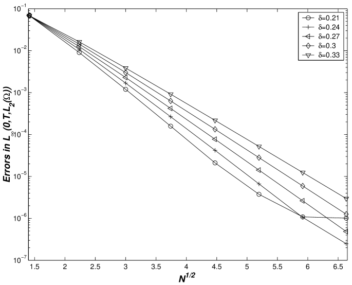
Figure 1: The errors $|||U_{h}-u|||_{60}$ plotted against $\sqrt{{\mathcal{N}}}$ for different choices of $\delta$, with $\alpha=-0.7$.

In Figure 2, for a fixed ${\mathcal{N}}=44$, we plot the errors against the parameter $\delta$ for different values of $\alpha$. We observe that values of $\delta$ in the neighborhood of the interval $[0.2,0.3]$ yields the best results.

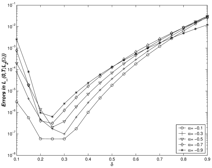
Figure 2: The errors $|||U_{h}-u|||_{60}$ plotted against $\delta$ for different values of $\alpha$ and fixed ${\mathcal{N}}=44$.

References

- [1] C-M. Chen, F. Liu, I. Turner and V. Anh, Numerical schemes and multivariate extrapolation of a two-dimensional anomalous sub-diffusion equation., Numer. Algor., 54, (2010) 1–21.
- [2] M. Cui, Compact finite difference method for the fractional diffusion equation, J. Comput. Phys., 228, (2009) 7792–7804.
- [3] M. Cui, Compact alternating direction implicit method for two-dimensional time fractional diffusion equation, J. Comput. Phys., 231, (2012) 2621–2633.
- [4] M. Cui, Convergence analysis of high-order compact alternating direction implicit schemes for the two-dimensional time fractional diffusion equation, Numer. Algor., 62, (2013) 383–409.
- [5] G.G. Gao and Z.Z. Sun, A box-type scheme for fractional sub-diffusion equation with Neumann boundary conditions, J. Comput. Phys., 230, (2011) 6061- 6074.
- [6] B. Jin, R. Lazarov and Z. Zhou, Error estimates for a semidiscrete finite element method for fractional order parabolic equations, SIAM J. Numer. Anal., 51, (2013) 445 -466.
- [7] A.A. Kilbas, H.M. Srivastava and J.J. Trujillo, Theory and Applications of Fractional Differential Equations, Volume 204 (North-Holland Mathematics Studies), 2006
- [8] T. A. M. Langlands, B. I. Henry, The accuracy and stability of an implicit solution method for the fractional diffusion equation, J. Comput. Phys., 205, (2005) 719–936.
- [9] F. Liu, C. Yang and K. Burrage, Numerical method and analytical technique of the modified anomalous subdiffusion equation with a nonlinear source term, Comput. Appl. Math., 231, (2009) 160-176.
- [10] A. M. Mathai, R. K. Saxena and H. J. Haubold, The H-Function: Theory and Applications, Springer, 2010.
- [11] W. Mclean, Regularity of solutions to a time-fractional diffusion equation, ANZIAM J., 52, (2010) 123 -138.
- [12] W. Mclean, Fast summation by interval clustering for an evolution equation with memory, SIAM J. Sci. Comput., 34, (2012) A3039-A3056.
- [13] W. Mclean and K. Mustapha, A second-order accurate numerical method for a fractional wave equation, Numer. Math., 105, (2007) 481–510.
- [14] W. McLean and K. Mustapha, Convergence analysis of a discontinuous Galerkin method for a sub-diffusion equation, Numer. Algo., 52, (2009) 69–88.
- [15] K. Mustapha, B. Abdallah and K.M. Furati, A discontinuous Petrov-Galerkin method for time-fractional diffusion equations, SIAM J. Numer. Anal., (2014), to appear.
- [16] K. Mustapha, An implicit finite difference time-stepping method for a sub-diffusion equation, with spatial discretization by finite elements, IMA J. Numer. Anal., 31, (2011) 719–739.
- [17] K. Mustapha, H. Brunner, H. Mustapha and D. Schötzau, An -version discontinuous Galerkin method for integro-differential equations of parabolic type, SIAM J. Numer. Anal., 49, (2011) 1369–1396.
- [18] K. Mustapha and W. McLean, Discontinuous Galerkin method for an evolution equation with a memory term of positive type, Math. Comp. 78, (2009) 1975–1995.
- [19] K. Mustapha and W. McLean, Piecewise-linear, discontinuous Galerkin method for a fractional diffusion equation, Numer. Algor., 56, (2011) 159–184.
- [20] K. Mustapha and W. McLean, Uniform convergence for a discontinuous Galerkin, time stepping method applied to a fractional diffusion equation, IMA J. Numer. Anal., 32, (2012) 906–925.
- [21] K. Mustapha and W. McLean, Superconvergence of a discontinuous Galerkin method for fractional diffusion and wave equations, SIAM J. Numer. Anal., 51, (2013) 491–515.
- [22] K. Mustapha and D. Schötzau, Well-posedness of version discontinuous Galerkin methods for fractional diffusion wave equations, IMA J. Numer. Anal., (2013), Accepted.
- [23] J. Quintana-Murillo and S.B. Yuste, An explicit difference method for solving fractional diffusion and diffusion-wave equations in the Caputo form, J. Comput. Nonlin. Dyn., 6, (2011) 021014.
- [24] D. Schötzau and C. Schwab, Time discretization of parabolic problems by the -version of the discontinuous Galerkin finite element method, SIAM J. Numer. Anal., 38, (2000) 837–875.
- [25] C. Schwab, and -Finite Element Methods – Theory and Applications in Solid and Fluid Mechanics, Oxford University Press, 1998.
- [26] I. Sokolov and J. Klafter, From diffusion to anomalous diffusion: A century after Einstein’s Brownian motion, Chaos, 15, (2005) 026103.
- [27] N. H. Sweilam, M. M. Khader and A. M. S. Mahdy, Crank-Nicolson finite difference method for solving time-fractional diffusion equation, J. Fract. Cal. Appl., 2 (2012) 1–9.
- [28] V. E. Tarasov, Fractional Dynamics: Applications of Fractional Calculus to Dynamics of Particles, Springer, Fields and Media (Nonlinear Physical Science), 2010.
- [29] H. Wang and K. Wang, An alternating-direction finite difference method for two-dimensional fractional diffusion equations, J. Comput. Phys., 230, (2011) 7830–7839.
- [30] S. B. Yuste and L. Acedo, An explicit finite difference method and a new von Neumann-type stability analysis for fractional diffusion equations, SIAM J. Numer. Anal., 42, (2005) 1862–1874.
- [31] S.B. Yuste and J. Quintana-Murillo, On three explicit difference schemes for fractional diffusion and diffusion-wave equations, Phys. Scripta T136, (2009) 014025.
- [32] Ya-nan Zhang and Zhi-zhong Sun, Alternating direction implicit schemes for the two-dimensional fractional sub-diffusion equation, J. Comput. Phys., 230, (2011) 8713–8728.
- [33] P. Zhuang, F. Liu, V. Anh and I. Turner, New solution and analytical techniques of the implicit numerical methods for the anomalous sub-diffusion equation, SIAM J. Numer. Anal., 46, (2008) 1079–1095.
- [34] P. Zhuang, F. Liu, V. Anh and I. Turner, Stability and convergence of an implicit numerical method for the nonlinear fractional reaction-subdiffusion process, IMA J. Appl. Math., 74, (2009) 645–667.