Abstract

A systematic analysis of possibilities for realizing single-field F-term axion monodromy inflation via the flux-induced superpotential in type IIB string theory is performed. In this well-defined setting the conditions arising from moduli stabilization are taken into account, where we focus on the complex-structure moduli but ignore the Kähler moduli sector. Our analysis leads to a no-go theorem, if the inflaton involves the universal axion. We furthermore construct an explicit example of F-term axion monodromy inflation, in which a single axion-like field is hierarchically lighter than all remaining complex-structure moduli.

1 Introduction

The recent announcements by BICEP2 [1] have triggered a fair amount of activity both in the interpretation of these results in comparison to the constraints by PLANCK, and in the theoretical realization of inflationary scenarios consistent with this data. However, for conclusive evidence in favor or against the BICEP2 results we still have to wait for improved estimates of the dust contribution and better statistics [2]. If the BICEP2 signal indeed contains B-modes of CMB origin, the large tensor-to-scalar ratio provides a sharp constraint for concrete models of inflation; in fact, most of the models proposed in the literature predict a much smaller ratio and would be ruled out. Moreover, the results of PLANCK show the absence of large non-Gaussianities, which is best fit by a model of single-field inflation.

It is well known that the dynamics of the inflaton, though in principle describable in an effective field theory, is sensitive to higher Planck-suppressed operators and therefore to the UV completion of the theory. String theory is believed to give a consistent quantum theory of gravity, and therefore it provides a suitable framework for reliably discussing inflation (for recent reviews see [3, 4, 5]).

String-theory compactifications to four space-time dimensions come with a multitude of initially massless scalar fields. These need to be stabilized for not immediately contradicting observations, such as the absence of fifth forces or the non-interference with the history of the cosmological evolution, like the cosmological moduli problem. In this approach, the universe starts at a generic point in a high-dimensional moduli space, followed by a period of fast rolling down of very massive scalar fields to their closest minimum, with one field being substantially lighter. This inflaton just happened to be in the slow-rolling phase for $N_{e}=60$ e-foldings before it reaches its minimum, after which it oscillates and thereby reheats the universe, initiating the next phase, the hot Big-Bang.

One of the recent new aspects in this scheme is due to BICEP2, which indicates a large tensor-to-scalar ratio, initially mentioned as $r=0.2$. The Lyth bound [6],

$$\begin{split}{\Delta\phi\over M_{\rm pl}}=O(1)\,\sqrt{r\over 0.01}\,,\end{split}$$ (1.1)

then implies a rolling of the inflaton $\phi$ over trans-Planckian distances $\Delta\phi>M_{\rm pl}$. For instance, for the above value $r=0.2$, the mass scale of inflation is at $M_{\rm inf}\sim 10^{16}\,$GeV, the Hubble scale of inflation at $H_{\rm inf}\sim 10^{14}\,$GeV and the mass of the inflaton is $m_{\theta}\sim 10^{13}\,$GeV. Moreover, a consequence of this large value for $r$ is that control over the scalar potential beyond the leading order term in $\phi/M_{\rm pl}$ is needed.

In string theory, there can be many higher-order corrections to the scalar potential. In the supergravity approximation we are studying here, these arise from corrections to the superpotential $W$ and to the Kähler potential $K$. These corrections are generically hard to control, unless one can invoke a symmetry which protects certain terms. In particular, some of the scalars in the low-energy theory may enjoy a continuous shift symmetry $\phi\to\phi+c$, which forbids perturbative corrections depending on $\phi$. (Non-perturbative corrections break the continuous shift symmetry to a discrete one.) These four-dimensional axions can descend from higher $p$-form fields in ten dimensions, but also geometric moduli of shift-symmetric backgrounds can show such a behavior. Recently discussed examples include the real parts of complex-structure moduli $\mathcal{U}=u+i\hskip 1.0ptv$ on a torus [7] or the deformation moduli $\xi$ of a $D7$-brane wrapping a transverse four-cycle of the internal manifold [8, 9]. On a generic Calabi-Yau manifold, such symmetries can also appear at special points in the moduli space, for instance in the large complex-structure limit.

In a string theory construction, after all other moduli have been stabilized, the leading-order non-perturbative contribution to the scalar potential of the axion is of the following general form

$$\begin{split}V=\lambda^{4}\left(1-\cos\Big{(}{\phi\over f}\Big{)}\right),\end{split}$$ (1.2)

where $f$ is the axion decay constant. Thus, for having trans-Planckian evolution, $f>1$ is required. This scenario is called natural inflation [10, 11], which in string theory is outside the regime of perturbative control [12]. In [13] it was investigated whether natural inflation can be realized in F-theory. Given the potential difficulties with natural inflation, one can consider multi-axion scenarios, where $f<1$ can be obtained by an alignment of axions [14, 15, 16, 17, 18], or by a multitude of axions called N-flation [19, 20, 21, 22]. (See also [23] for work on assisted inflation, and [24, 25] for M-flation).

Another approach, still allowing for some control over the higher-order corrections, is axion monodromy inflation [26, 27], for which a field-theory version has been proposed in [28, 29]. For a recent review see [30]. In a corresponding string-theoretic embedding, D-branes or background fluxes break the shift symmetry, but in a somewhat soft way so that the finite interval for the axion $0\leq\phi<2\pi/f$ is unwrapped while in each covering interval the physics is unchanged. Moreover, each time the axion completes a period, the energy density increases by a certain amount. Realizations of this scenario with D-branes (see e.g. [31]) usually involve the introduction of brane/anti-brane pairs in order to satisfy tadpole cancellation. However, configurations with anti-branes break supersymmetry explicitly and therefore make them difficult to control. In fact, in [32] it has been shown that for $D5$-brane/anti-brane scenarios the backreaction is large and cannot be neglected.

Recently it has been proposed to realize the scenario of axion monodromy inflation via the F-term scalar potential induced by background fluxes [33]. This has the advantage that supersymmetry is broken spontaneously by the very same effect by which usually moduli are stabilized. Moreover, this scenario is generic in the sense that the scalar potential for the axions arises from the type II Ramond-Ramond field strengths $F_{p+1}=dC_{p}+H\wedge C_{p-2}$, which involve the gauge potentials $C_{p}$ explicitly.

For realizing F-term monodromy inflation in string theory, a number of proposals have been made. In [34] a scenario based on the universal axion $C_{0}$ was discussed, where it was argued that this axion provides a natural mechanism for reheating to occur mainly into Standard Model degrees of freedom. In [8, 35] the inflaton was given by a deformation modulus of a $D7$-brane which was argued to enjoy a shift symmetry (at special points in the moduli space). In [9] the axion was identified with an open-string modulus, namely the superpartner in the Higgs sector of the MSSM. In the much-discussed example of [7] (see also [36]), the axion was considered to be the Kalb-Ramond field $B$ integrated over an internal two-cycle, whereas in [33] it was proposed to use a $D7$-brane Wilson line modulus. Note that initially the latter model requires a continuous one-cycle in the internal four-cycle wrapped by the $D7$-brane, which becomes twisted by turning on geometric flux. This means that from the global string model-building perspective, these scenarios are far less understood and more work is needed to make them well-defined and consistent string backgrounds. In [37] non-geometric fluxes were employed and the inflaton was given by a Kähler modulus. For an example of inflation realized in a warped resolved conifolds see [38].

We note that these proposals of F-term axion monodromy inflation have in common that they were developed on the level of principle scenarios, where statements such as “in the huge landscape of flux compactifications we expect to find models with a certain quantity to be parametrically small” can often be found. In this paper, we start a more systematic study of realizing single-field flux-induced F-term axion monodromy inflation, taking into account the interplay with moduli stabilization. Note that moduli stablization is at the core of reliably realizing such models in string theory, as in single-field inflation, all other moduli need to get a mass larger than the Hubble scale $H_{\rm inf}$. Therefore, the F-term giving rise to the axion monodromy, at the same time has to lead to a controllable mass hierarchy between the axion and all the other moduli appearing in it. Of course, there can be even more moduli beyond the ones directly appearing in the axionic F-term, for which at a later stage the issue has to be addressed, as well. To be as precise as possible, in this paper we will work in the well defined, i.e. also restricted, setting of type IIB three-form flux compactifications, for which the relevant F-term depends on the complex-structure moduli and axio-dilaton.

This paper is organized as follows. In section 2, we describe the technical challenges one is facing when trying to realize single large-field axion inflation in string theory. In section 3, we recall the main aspects of flux compactifications in type IIB orientifolds and discuss the problem of keeping an axion massless. In section 4, we present some examples which show certain features of flux vacua with massless modes. We find that some of the desired properties can indeed be realized, but to have a single massless axionic mode is a true challenge. In section 5, we analyze this situation from a more general point of view and prove a no-go theorem for models where the massless mode is a linear combination of axions involving $C_{0}$. We furthermore discuss conditions for unconstrained axion-like fields containing only complex-structure moduli. Here the analysis turns out to be more involved: for certain cases we can still prove no-go theorems, but we also construct a concrete working model. The reader interested only in the final result may first read section 2, and then go directly to section 5. Section 6 contains our conclusions.

2 String-theoretic challenges of axion inflation

Although string theory in principle provides all the necessary ingredients, in a concrete string compactification with many moduli it is challenging to find a model with large masses for all moduli fields except one. That means, it is difficult to disentangle the scale of the moduli masses from the mass of a single inflaton. In particular, string theory is only well-understood for backgrounds where supersymmetry is broken spontaneously. Hence, to find only one light modulus one typically needs to split the masses of the scalar fields residing in the same supermultiplet.

Moreover, as mentioned above, for large scalar-to-tensor ratios $r$ one needs to have control over the scalar potential for $\phi/M_{\rm pl}>1$. Let us explain in a bit more detail what this means for a flux-induced scalar potential already at tree level. (Higher-order corrections could of course also induce an $\eta$-problem, but we ignore this effect for the moment.) Thus, assume that after fixing all remaining moduli, we end up with the following effective Lagrangian for the lightest modulus in four dimensions

$$\begin{split}{\cal L}={1\over 2}\partial_{\mu}\phi\,\partial^{\mu}\phi-V(\phi)\,,\end{split}$$ (2.1)

where the field $\phi$ has been normalized such that it has a canonical kinetic term. The tree-level potential takes the general form

$$\begin{split}V(\phi)=M_{\rm pl}^{4}\,\sum_{n\geq 2}a_{n}\left({\phi\over M_{\rm pl}}\right)^{n},\end{split}$$ (2.2)

when Taylor-expanded around one of its minima. In the small-field regime $\phi\ll M_{\rm pl}$, higher-order terms are suppressed and the scalar potential in (2.1) can be approximated by the quadratic term in the vicinity of the minimum. However, if the quadratic potential gives rise to inflation for $\phi\gg M_{\rm pl}$, one cannot study the potential only around a minimum but needs to take into account all higher terms in the expansion (2.2) of the tree-level potential. Let us be somewhat more concrete and set $M_{\rm pl}=1$ for convenience, so that large field means $\phi>1$. If we had for instance a flux-induced scalar potential of the form

$$\begin{split}V(\phi)=F\left({\phi\over f}\right)=m_{2}\left(\phi\over f\right)^{2}+m_{3}\left(\phi\over f\right)^{3}+\ldots\end{split}$$ (2.3)

with $f>1$, we could approximate $V(\phi)$ even in the trans-Planckian regime $1<\phi\ll f$ by just the quadratic term. This is what happens for the non-perturbative potential (1.2). In our situation, one would expect the parameter $f$ to be a combination of background fluxes. But this is not clear a priori, and the question arises whether in a general string construction the potential for the lightest field involves a parameter $f$ which indeed depends on the fluxes.

Concerning the higher-order perturbative corrections to the tree-level potential (2.2), these can be controlled if one invokes the shift symmetry of an axionic field. This symmetry is usually broken in a controlled way by having an extra contribution to the energy density, giving rise to an axion monodromy. The main task therefore is to find minima of the scalar potential such that an axion, or an axion-like field, becomes the parametrically lightest scalar, whose dynamics, after integrating out all the heavier fields, is governed by a simple $\phi^{q}$ effective potential. As proposed in [39, 7], $q$ could also be a rational number.

The certainly best understood scenario for moduli stabilization in string theory are type IIB orientifold compactifications on Calabi-Yau three-folds, where the axio-dilaton and the complex-structure moduli are stabilized by a three-form flux-induced tree-level potential, while the Kähler moduli are frozen at subleading order in the overall volume modulus ${\cal V}$ by a combination of higher-order and non-perturbative effects [40, 41]. Recall also that for type IIB orientifold models with three-form fluxes, the continuous shift symmetry of the universal axion $C_{0}$ is broken to a discrete one, which is embedded into the $SL(2,\mathbb{Z})$ S-duality of type IIB. The flux-induced scalar potential preserves this duality since $SL(2,\mathbb{Z})$ also acts on the discrete fluxes accordingly, thus splitting the configuration space into different branches. However, choosing a concrete flux background, the shift symmetry gets spontaneously broken and in the corresponding branch one realizes the above mentioned axionic monodromy.

In the following, we investigate whether the landscape of minima of the flux-induced scalar potential admits solutions with the following properties:

1. All moduli are stabilized such that one axion is parametrically lighter than the other moduli and the axion admits a shift symmetry.

2. For this inflaton candidate, the tree-level scalar potential in the trans-Planckian regime still realizes large-field inflation.

The axion or axion-like fields we consider are mainly the universal axion and the real part of the complex-structure moduli, i.e. we work in the large complex-structure limit ${\rm Im}\>\mathcal{U}=v\to\infty$.

For a generic choice of background fluxes, all complex-structure moduli and the axio-dilaton are stabilized at isolated points, and the kinetic terms as well as the mass matrix in the minimum involve off-diagonal components. Therefore, it is not an easy task to obtain general information about the eigenvalues and eigenstates in the canonically normalized basis. Our approach to the first requirement from above is to first try to keep precisely one axionic mode unconstrained by a non-generic choice of (large) fluxes. In a second step, we give a small mass to this axion by turning on some additional hierarchically-smaller fluxes. This means that we have parametric control over the flux-induced mass of the axion by identifying a flux-dependent parameter controlling the hierarchy between the mass scales of the heavy moduli and the inflaton.

One could think, and in fact this argument has often been used in the literature, that the plenitude of discrete fluxes allows to realize essentially any property one desires at some point in the landscape. Thus, part of our analysis involves the important question which parameters can be dialed small or big by an appropriate choice of fluxes.

3 Moduli stabilization by fluxes

In this section, we first recall some facts about the scalar potential induced by three-form fluxes in type IIB orientifold models [42, 43]. In the second part, we draw general conclusions about the possibility of stabilizing all moduli but leaving one axion massless.

3.1 Flux-induced potential

Let us start by recalling the form of the complex three-form flux in type IIB supergravity as

$$\begin{split}G_{3}=F_{3}+\tau\hskip 1.0ptH_{3}\,,\end{split}$$ (3.1)

which is expressed in terms of the NS-NS flux $H_{3}$, the R-R flux $F_{3}$ and the universal axio-dilaton

$$\begin{split}\tau=C_{0}+i\hskip 1.0pte^{-\phi}=c+i\hskip 1.0pts\,.\end{split}$$ (3.2)

When compactifying type IIB string theory on a six-dimensional manifold $\mathcal{X}$ and allowing for non-trivial fluxes, the ten-dimensional action corresponding to $G_{3}$ takes the following form in Einstein-frame

$$\begin{split}S=-\frac{1}{4\hskip 1.0pt\kappa_{10}^{2}\hskip 1.0pt{\rm Im}(\tau)}\int_{\mathbb{R}^{3,1}\times\mathcal{X}}G_{3}\wedge\star_{10}\hskip 1.0pt\overline{G}_{3}\,,\end{split}$$ (3.3)

where $\overline{G}_{3}$ denotes the complex conjugate of $G_{3}$ and where the gravitational coupling reads $\kappa_{10}^{2}={1\over 2}(2\pi)^{7}(\alpha^{\prime})^{4}$. Apart from the four-dimensional kinetic terms, the action (3.3) contains a contribution to the tadpole for the four-form $C_{4}$ and a contribution to the scalar potential.

D-term contribution

Let us discuss the tadpole contribution contained in (3.3) first, which is proportional to

$$\begin{split}N_{\rm flux}=\frac{1}{(2\pi)^{4}(\alpha^{\prime})^{2}}\int_{\mathcal{X}}H_{3}\wedge F_{3}\,.\end{split}$$ (3.4)

For studying this expression, we choose an integral basis $\{A^{\Lambda},B_{\Sigma}\}$ of $H_{3}(X,\mathbb{Z})$ with the intersections $A^{\Lambda}\cap A^{\Sigma}=B_{\Lambda}\cap B_{\Sigma}=0$ and $A^{\Lambda}\cap B_{\Sigma}=\delta^{\Lambda}_{\Sigma}$, where $\Lambda,\Sigma=0,\dots,h^{2,1}$. In terms of the Poincaré dual basis $\{\alpha_{\Lambda},\beta^{\Lambda}\}$ of $H^{3}(X,\mathbb{Z})$, the covariantly constant $(3,0)$-form can be expanded as

$$\begin{split}\Omega_{3}=X^{\Lambda}\,\alpha_{\Lambda}-F_{\Lambda}\,\beta^{\Lambda},\end{split}$$ (3.5)

where the periods $X^{\Lambda}$ and $F_{\Lambda}$ are functions of the complex-structure moduli ${\cal U}^{i}$, with $i=1,\dots,h^{2,1}$. In terms of $\Omega_{3}$, the periods can be determined as follows

$$\begin{split}X^{\Lambda}=\int_{A^{\Lambda}}\Omega_{3}\,,\hskip 50.0ptF_{\Lambda}=\int_{B_{\Lambda}}\Omega_{3}\,.\end{split}$$ (3.6)

Due to the Bianchi identities and the quantization conditions of the three-form fluxes, $H_{3}$ and $F_{3}$ can be expressed as integer linear combinations (in cohomology)

$$\begin{split}\begin{array}[]{lcl@{\hspace{70pt}}lcl}\tfrac{1}{(2\pi)^{2}\alpha^{\prime}}\,H_{3}&=&h_{\Lambda}\,\beta^{\Lambda}+\overline{h}^{\Lambda}\,\alpha_{\Lambda}\,,\hfil\hskip 70.&h_{\Lambda},\overline{h}^{\Lambda}&\in&\mathbb{Z}\,,\\[6.0pt] \tfrac{1}{(2\pi)^{2}\alpha^{\prime}}\,F_{3}&=&f_{\Lambda}\,\beta^{\Lambda}+\overline{f}^{\Lambda}\,\alpha_{\Lambda}\,,\hfil\hskip 70.&f_{\Lambda},\overline{f}^{\Lambda}&\in&\mathbb{Z}\,.\end{array}\end{split}$$ (3.7)

The complex three-form flux defined in equation (3.1) can therefore be written in the following way

$$\begin{split}\tfrac{1}{(2\pi)^{2}\alpha^{\prime}}\,G_{3}=e_{\Lambda}\hskip 1.0pt\beta^{\Lambda}+m^{\Lambda}\hskip 1.0pt\alpha_{\Lambda}\,,\hskip 60.0pt\begin{array}[]{lcl}e_{\Lambda}&=&\tau\,h_{\Lambda}+f_{\Lambda}\,,\\[6.0pt] m^{\Lambda}&=&\tau\,\overline{h}^{\Lambda}+\overline{f}^{\Lambda}\,,\end{array}\end{split}$$ (3.8)

and in this notation the contribution to the $C_{4}$-tadpole shown in (3.4) becomes

$$\begin{split}N_{\rm flux}=m\times e=\overline{h}^{\Lambda}\hskip 1.0ptf_{\Lambda}-\overline{f}^{\Lambda}\hskip 1.0pth_{\Lambda}\,.\end{split}$$ (3.9)

Since this term contributes to the NS-NS $D3$-brane tadpole cancellation condition, it should be considered as a D-term.

F-term contribution

We now turn to the contribution to the scalar potential contained in (3.3). It corresponds to the imaginary self-dual part $G^{+}_{3}$ of $G_{3}$ which, after going to Einstein frame reads

$$\begin{split}V_{F}=-\frac{M_{\rm pl}^{4}}{4\pi}\,\frac{e^{\phi}}{\mathcal{V}^{2}}\,\frac{1}{(2\pi)^{4}(\alpha^{\prime})^{2}}\int_{\mathcal{X}}G_{3}^{+}\wedge\star_{6}\hskip 1.0pt\overline{G}_{3}^{+}\,.\end{split}$$ (3.10)

Here, $\mathcal{V}$ denotes the volume of the compactification manifold in units of the string length $2\pi\sqrt{\alpha^{\prime}}$, and the four-dimensional Planck mass was defined as $M_{\rm pl}^{2}={\cal V}\,(2\pi\alpha^{\prime})^{-1}$. Employing matrix notation together with the definitions in (3.8), the potential (3.10) can be written as

$$\begin{split}V_{F}=-\frac{M_{\rm pl}^{4}}{4\pi}\,\frac{1}{\mathcal{V}^{2}\,{\rm Im}\hskip 1.0pt\tau}\,(e+m\hskip 1.0pt\overline{\cal N})({\rm Im}{\cal N})^{-1}(\overline{e}+{\cal N}\hskip 1.0pt\overline{m})\,.\end{split}$$ (3.11)

The matrix $\mathcal{N}_{\Lambda\Sigma}$ appearing here is called the period matrix, and with $F_{\Lambda\Sigma}=\partial F_{\Lambda}/\partial X_{\Sigma}$ it is defined as

$$\begin{split}{\cal N}_{\Lambda\Sigma}=\overline{F}_{\Lambda\Sigma}+2i\,\frac{{\rm Im}(F_{\Lambda\Gamma})X^{\Gamma}\,{\rm Im}(F_{\Sigma\Delta})X^{\Delta}}{X^{\Gamma}\,{\rm Im}(F_{\Gamma\Delta})X^{\Delta}}\,.\end{split}$$ (3.12)

Since this matrix depends on the complex-structure moduli, also the scalar potential $V_{F}$ in (3.11) is a function of ${\cal U}^{i}$ and $\tau$. In the physical domain of the complex-structure moduli space, the matrix ${\rm Im}\hskip 1.0pt{\cal N}$ is regular and negative definite, so that the potential $\eqref{scalarpota}$ is positive definite. We also observe that there is an obvious candidate for a minimum of the scalar potential (3.11) at

$$\begin{split}e_{\Lambda}+m^{\Sigma}\,\overline{\cal N}_{\Sigma\Lambda}=0\,,\end{split}$$ (3.13)

corresponding to an imaginary self-dual $G_{3}$ flux. Note that the latter satisfies $G^{(1,2)}+G^{(3,0)}=0$.

Let us also mention the paper [44], where it was shown that (3.11) can be understood as the F-term scalar potential. In particular, consider the following superpotential

$$\begin{split}W=\frac{M^{2}_{\rm pl}}{\sqrt{2\pi}}\int_{\mathcal{X}}\Omega_{3}\wedge{G_{3}\over(2\pi)^{2}\alpha^{\prime}}=\frac{M^{2}_{\rm pl}}{\sqrt{2\pi}}\left(e_{\Lambda}X^{\Lambda}+m^{\Lambda}F_{\Lambda}\right),\end{split}$$ (3.14)

together with the tree-level Kähler potential

$$\begin{split}\mathcal{K}=-\log\Bigl{(}-i\hskip 1.0pt(\tau-\overline{\tau})\Bigr{)}-2\log\mathcal{V}-\log\left(-i\int_{\mathcal{X}}\Omega_{3}\wedge\overline{\Omega}_{3}\right).\end{split}$$ (3.15)

Employing then for instance the identities $F_{\Lambda}={\cal N}_{\Lambda\Sigma}X^{\Sigma}$ and $D_{i}F_{\Lambda}=\overline{{\cal N}}_{\Lambda\Sigma}D_{i}X^{\Sigma}$, one can express the scalar potential (3.11) as

$$\begin{split}V_{F}=M_{\rm pl}^{4}\,e^{\mathcal{K}}\left[G^{i\overline{j}}\,D_{i}WD_{\overline{j}}\overline{W}+G^{\tau\overline{\tau}}\,D_{\tau}WD_{\overline{\tau}}\overline{W}\right].\end{split}$$ (3.16)

Let us emphasize that since in (3.16) the contribution from the Kähler moduli $T_{a}$ contained in $\mathcal{V}$ has canceled against the $-3|W|^{2}$ term, this scalar potential is of no-scale type. Furthermore, due to the positivity of $|DW|^{2}$, the conditions for the global minimum (3.13) correspond to the vanishing of the F-terms $D_{i}W=0$ and $D_{S}W=0$. Therefore, supersymmetry can only be broken by the Kähler moduli if $D_{T_{a}}W=(\partial_{T_{a}}K)\,W\neq 0$.

Prepotential

In this paper we consider the flux-induced scalar potential for compactifications on Calabi-Yau manifolds in the large complex-structure regime. Employing mirror symmetry, this means that we take into account only the tree-level contribution to the prepotential while neglecting all world-sheet instanton corrections.

In special geometry, the holomorphic three-form (3.5) defines the homogeneous coordinates $X^{\Lambda}$ and the derivatives $F_{\Lambda}=\partial_{\Lambda}F$ of a prepotential $F$. In the large complex-structure regime, the prepotential has the simple form

$$\begin{split}{F}={\kappa_{ijk}{X}^{i}{X}^{j}{X}^{k}\over{X}^{0}}\,,\end{split}$$ (3.17)

where $\kappa_{ijk}$ with $i,j,k=1,\ldots,h^{2,1}$ denote the triple intersection numbers of the mirror Calabi-Yau manifold. The complex-structure moduli ${\cal U}^{i}\equiv u^{i}+i\hskip 1.0ptv^{i}$ are defined via

$$\begin{split}\begin{array}[]{lcl@{\hspace{70pt}}lcl}X^{0}&=&1\,,\hfil\hskip 70.&F_{0}&=&-\kappa_{ijk}\,{\cal U}^{i}\,{\cal U}^{j}\,{\cal U}^{k}\,,\\[8.0pt] X^{i}&=&{\cal U}^{i}\,,\hfil\hskip 70.&F_{i}&=&3\,\kappa_{ijk}\,{\cal U}^{j}\,{\cal U}^{k}\,.\end{array}\end{split}$$ (3.18)

As mentioned in (3.15), the tree-level Kähler potential for the complex-structure moduli reads

$$\begin{split}K_{\rm cs}=-\log\left(-i\int_{\mathcal{X}}\Omega_{3}\wedge\overline{\Omega}_{3}\right)=-\log\left(\kappa_{ijk}v^{i}\,v^{j}\,v^{k}\right),\end{split}$$ (3.19)

which only depends on the imaginary parts of the ${\cal U}^{i}$ and is therefore invariant under continuous shifts $u^{i}\to u^{i}+c^{i}$. The period matrix for the prepotential (3.17) takes the following form

$$\begin{split}\begin{array}[]{lcllcl}{\rm Im}\,\mathcal{N}_{ij}&=&4\,\kappa\,G_{i\overline{j}}\;,&{\rm Re}\,\mathcal{N}_{ij}&=&6\,\kappa_{ijk}\,u^{k}\;,\\[5.12149pt] {\rm Im}\,\mathcal{N}_{i0}&=&-4\,\kappa\,G_{i\overline{j}}\,u^{j}\;,&{\rm Re}\,\mathcal{N}_{i0}&=&-3\,\kappa_{ijk}\,u^{j}u^{k}\;,\\[2.27621pt] {\rm Im}\,\mathcal{N}_{00}&=&\kappa\,\Bigl{(}1+4\,G_{i\overline{j}}\,u^{i}u^{j}\Bigr{)}\;,&{\rm Re}\,\mathcal{N}_{00}&=&2\,\kappa_{ijk}\,u^{i}u^{j}u^{k}\;,\end{array}\end{split}$$ (3.20)

where the Kähler metric computed from (3.19) reads

$$\begin{split}G_{i\overline{j}}=-\frac{3}{2}\>\frac{\kappa_{ij}}{\kappa}+\frac{9}{4}\frac{\kappa_{i}\kappa_{j}}{\kappa^{2}}\,,\end{split}$$ (3.21)

and where we have defined

$$\begin{split}\kappa=\kappa_{ijk}\,v^{i}v^{j}v^{k}\,,\hskip 40.0pt\kappa_{i}=\kappa_{ijk}\,v^{j}v^{k}\,,\hskip 40.0pt\kappa_{ij}=\kappa_{ijk}\,v^{k}\,.\end{split}$$ (3.22)

Note that in the physical domain, besides the requirement $s>0$ for the dilaton, the Kähler metric $G_{i\overline{j}}$ on the complex-structure moduli space has to be positive definite.

Remark

The prepotential (3.17) is subject to perturbative and non-perturbative corrections, which take the following general form (see for instance [45]) 

$$\begin{split}\widetilde{F}=F+\frac{1}{2}\hskip 1.0pta_{ij}X^{i}X^{j}+b_{i}X^{i}X^{0}+\frac{1}{2}\hskip 1.0ptc\bigl{(}X^{0}\bigr{)}^{2}+F_{\rm inst.}\,.\end{split}$$ (3.23)

Here, the constants $a_{ij}$ and $b_{i}$ are rational real numbers, while $c=i\hskip 1.0pt\gamma$ is purely imaginary. Ignoring the non-perturbative corrections, the period matrix following from (3.23) is found to be of the following form

$$\begin{split}\begin{array}[]{lcllcl}{\rm Re}\,\widetilde{\mathcal{R}}_{00}&=&\displaystyle 2\hskip 1.0pt\kappa_{ijk}u^{i}u^{j}u^{k}-\frac{18\hskip 1.0pt\gamma}{8\kappa-\gamma}\,\kappa_{i}u^{i}\,,\\[15.0pt] {\rm Re}\,\widetilde{\mathcal{R}}_{0i}&=&\displaystyle-3\hskip 1.0pt\kappa_{ijk}u^{j}u^{k}+b_{i}+\frac{9\hskip 1.0pt\gamma}{8\kappa-\gamma}\,\kappa_{i}\,,\\[15.0pt] {\rm Re}\,\widetilde{\mathcal{R}}_{ij}&=&\displaystyle 6\hskip 1.0pt\kappa_{ijk}u^{k}+a_{ij}\,,\\[15.0pt] {\rm Im}\,\widetilde{\mathcal{N}}_{00}&=&\displaystyle\frac{8\kappa^{2}-2\kappa\hskip 1.0pt\gamma-\gamma^{2}}{8\kappa-\gamma}-6\left[\kappa_{ij}-\frac{12}{8\kappa-\gamma}\hskip 1.0pt\kappa_{i}\kappa_{j}\right]u^{i}u^{j}\,,\\[15.0pt] {\rm Im}\,\widetilde{\mathcal{N}}_{0i}&=&\displaystyle 6\left[\kappa_{ij}-\frac{12}{8\kappa-\gamma}\hskip 1.0pt\kappa_{i}\kappa_{j}\right]u^{j}\,,\\[15.0pt] {\rm Im}\,\widetilde{\mathcal{N}}_{ij}&=&\displaystyle-6\left[\kappa_{ij}-\frac{12}{8\kappa-\gamma}\hskip 1.0pt\kappa_{i}\kappa_{j}\right]\,.\end{array}\end{split}$$ (3.24)

From these explicit expressions it follows that when computing the scalar potential (3.11), the real corrections $a_{ij}$ and $b_{i}$ can be incorporated by the following shift in the fluxes

$$\begin{split}\begin{array}[]{lcl@{\hspace{50pt}}lcl}\widetilde{h}_{0}&=&h_{0}+b_{i}\hskip 1.0pt\overline{h}^{i}\,,\hfil\hskip 50.&\widetilde{h}_{i}&=&h_{i}+a_{ij}\hskip 1.0pt\overline{h}^{j}+b_{i}\hskip 1.0pt\overline{h}^{0}\,,\\[5.0pt] \widetilde{f}_{0}&=&f_{0}+b_{i}\hskip 1.0pt\overline{f}^{i}\,,\hfil\hskip 50.&\widetilde{f}_{i}&=&f_{i}+a_{ij}\hskip 1.0pt\overline{f}^{j}+b_{i}\hskip 1.0pt\overline{f}^{0}\,.\end{array}\end{split}$$ (3.25)

The purely imaginary contribution $c=i\hskip 1.0pt\gamma$ corresponds to $\alpha^{\prime}$-corrections to the Kähler potential for the Kähler moduli in a mirror-dual setting. In the large complex-structure regime we are employing here,

$$\begin{split}\kappa_{ijk}v^{i}v^{j}v^{k}\gg{\rm Im}\hskip 1.0ptc\hskip 50.0pt\Leftrightarrow\hskip 40.0pt\kappa\gg\gamma\,,\end{split}$$ (3.26)

these corrections can be neglected in the period matrix (3.24). Similarly, in this regime also the non-perturbative corrections $F_{\rm inst.}$ are negligible.

To summarize, for computing the scalar potential (3.11) in the large complex-structure limit, corrections to the prepotential can be incorporated by a rational shift in the fluxes. Since our subsequent analysis will not depend crucially on the precise values of these fluxes, we will work with the classical prepotential (3.17).

3.2 Massless axions

We now want to study moduli stabilization for the flux-induced scalar potential (3.11). In particular, we are interested in keeping one of the axions massless while all other moduli, particularly its saxionic partner, become massive.

Problem of mass splitting the axio-dilaton

Let us first discuss the simple case of the complex axio-dilaton modulus. Say we are in the generic situation that for a choice of fluxes the conditions (3.13) fix the complex-structure moduli $\mathcal{U}^{i}$ and the axio-dilaton $\tau$ completely. Expanding then $\tau=c+i\hskip 1.0pts$ around the background values in the minimum, $c=\overline{c}+\delta c$ and $s=\overline{s}+\delta s$, from (3.11) we can determine the mass terms for these two scalars from

$$\begin{split}V_{F}\sim\bigl{[}(\delta c)^{2}+(\delta s)^{2}\bigr{]}\Bigl{[}(h+\overline{h}\,\overline{\cal N})({\rm Im}\hskip 1.0pt{\cal N})^{-1}(h+{\cal N}\,\overline{h})\Bigr{]}_{0}\,,\end{split}$$ (3.27)

where the expression in the second bracket has to be evaluated in the minimum. This formula suggests that, even for non-supersymmetric minima, the axion and the dilaton are degenerate in mass.

Therefore, it seems that from the fluxes alone one cannot get the desired mass splitting. The only loop-hole in this argument is that we ignored possible mixing terms with the complex-structure moduli of the form $M^{2}_{si}\,(\delta s)(\delta v^{i})$. Examples where such effects can become substantial are models where the fluxes do not stabilize all moduli but only certain combinations of the axio-dilaton and the complex-structure moduli. We will construct examples for a simple toroidal orbifold in section 4.

The problem of keeping just $C_{0}$ massless

In order to keep the universal axion $c=C_{0}$ massless, we require that the constraints (3.13) do not involve $c$. Of course, this is only a sufficient condition, and it might happen that the axion is constrained but no mass term is generated. In this paper, we do not consider the latter possibility and require the axion to be unconstrained. Writing then out (3.13), we find the following $(2h^{2,1}+2)$ real conditions

$$\begin{split}c\left(h_{\Lambda}+{\rm Re}{\cal N}_{\Lambda\Sigma}\,\overline{h}^{\Sigma}\right)+s\left({\rm Im}{\cal N}_{\Lambda\Sigma}\,\overline{h}^{\Sigma}\right)+\left(f_{\Lambda}+{\rm Re}{\cal N}_{\Lambda\Sigma}\,\overline{f}^{\Sigma}\right)&=0\,,\\ -c\left({\rm Im}{\cal N}_{\Lambda\Sigma}\,\overline{h}^{\Sigma}\right)+s\left(h_{\Lambda}+{\rm Re}{\cal N}_{\Lambda\Sigma}\,\overline{h}^{\Sigma}\right)-\left({\rm Im}{\mathcal{N}}_{\Lambda\Sigma}\,\overline{f}^{\Sigma}\right)&=0\,.\end{split}$$ (3.28)

Note that the complex-structure dependent coefficients of $c$ and $s$ are the same, so that keeping just $c$ unconstrained in the first relation directly implies that also the dilaton $s$ is unconstrained. Moreover, in this case the second relation in (3.28) implies

$$\begin{split}{\rm Im}\hskip 1.0pt{\cal N}_{\Lambda\Sigma}\,\overline{h}^{\Sigma}=0\,,\hskip 50.0pt{\rm Im}\hskip 1.0pt{\cal N}_{\Lambda\Sigma}\,\overline{f}^{\Sigma}=0\,,\end{split}$$ (3.29)

which in the physical domain of the complex-structure moduli space means that all fluxes $\overline{f}^{\Sigma}$ and $\overline{h}^{\Sigma}$ need to vanish. But via the first relation in (3.28) that implies $f_{\Lambda}=h_{\Lambda}=0$. Therefore, we conclude that the universal axion $c$ can only be unconstrained in the minimum of the scalar potential if either all fluxes vanish (trivial case), or if the complex-structure moduli are stabilized at the boundary of the physical domain. Again, a loophole in this argument is that the inflaton might not be $c$ directly but a combination with axion-like states, i.e. a combination of $c$ and $u^{i}$.

4 Examples with parametrically light moduli

In this section, we consider simple non-supersymmetric minima of the flux potential, which show some features of points in the landscape. First, we look at the isotropic torus and investigate moduli stabilization with a massless state containing both saxionic and axionic components. Second, we consider purely axionic unconstrained states on the non-isotropic torus and on ${\rm IP}_{1,1,2,2,2}[8]$.

4.1 The isotropic torus

Our conventions for the toroidal examples can be found in the appendix A.1 and are identical to those of [46]. For the model discussed in this section, we find that one of the moduli remains massless. However, as it will be discussed, by turning on additional fluxes, also the remaining modulus can get a small mass. This example, though not perfect, is presented to demonstrate which parameters in a concrete flux vacuum can be dialed small by an appropriate choice of fluxes. One of the results is that some parameters turn out to be flux independent.

A model with one massless state

Let us consider the isotropic limit of the toroidal orbifold model, that is $u=u^{1}=u^{2}=u^{3}$ and $v=v^{1}=v^{2}=v^{3}$, for which the Minkowski minima are determined by the constraints (3.13). For these concrete expressions, we investigate whether it is possible to have a linear combination of the axions $c$ and $u$ unconstrained in the physical domain $v<0$ and $s>0$. We find that this is only possible for the trivial choice of fluxes. Therefore, there does not exist any minimum of the flux-induced scalar potential with one axion staying massless and the remaining three moduli being massive.

However, in order to illustrate the underlying structure and to develop some tools for later on, let us consider a model determined by the following choice of fluxes

$$\begin{split}e_{0}=\tau\hskip 1.0pth_{0}+f_{0}\,,\hskip 50.0ptm^{0}=\tau\hskip 1.0pt\overline{h}_{0}+\overline{f}_{0}\,,\end{split}$$ (4.1)

and $h_{1}$, $f_{1}$, $\overline{h}_{1}$, $\overline{f}_{1}$ vanishing. The moduli are stabilized as

$$\begin{split}u=0\,,\qquad c=-{f_{0}h_{0}+\overline{f}_{0}\overline{h}_{0}\hskip 1.0ptv^{6}\over h_{0}^{2}+\overline{h}_{0}^{2}v^{6}}\,,\qquad s={\overline{f}_{0}h_{0}-f_{0}\overline{h}_{0}\over h_{0}^{2}+\overline{h}_{0}^{2}v^{6}}\,v^{3}\,,\end{split}$$ (4.2)

that is three out of four moduli are fixed while one modulus stays unconstrained. Note that in order to be in the physical domain $v<0$ and $s>0$, we have to require that

$$\begin{split}\kappa=\overline{f}_{0}\hskip 1.0pth_{0}-f_{0}\hskip 1.0pt\overline{h}_{0}<0\,,\end{split}$$ (4.3)

and therefore (3.9) satisfies $N_{\rm flux}>0$. The unconstrained mode is a combination of the $(c,s,v)$ moduli, i.e. it is a mixture of an axion with two saxions. We introduce canonically normalized fluctuations $\{\delta\tilde{c},\delta\tilde{s},\delta\tilde{v},\delta\tilde{u}\}$, which are related to fluctuations of the stringy variables via

$$\begin{split}\delta\tilde{c}={1\over 2s}\,\delta c\,,\qquad\delta\tilde{s}={1\over 2s}\,\delta s\,,\qquad\delta\tilde{v}={\sqrt{3}\over 2v}\,\delta v\,,\qquad\delta\tilde{u}={\sqrt{3}\over 2v}\,\delta u\,.\end{split}$$ (4.4)

The normalized mass eigenstates of this model are

$$\begin{split}\phi_{1}&=-\frac{\sqrt{3}h_{0}\overline{h}_{0}v_{0}^{3}}{h_{0}^{2}+\overline{h}_{0}^{2}v_{0}^{6}}\,\delta\tilde{c}+\frac{\sqrt{3}(h_{0}-\overline{h}_{0}v_{0}^{3})(h_{0}+\overline{h}_{0}v_{0}^{3})}{2(h_{0}^{2}+\overline{h}_{0}^{2}v_{0}^{6})}\,\delta\tilde{s}+{1\over 2}\,\delta\tilde{v}\,,\\[2.84544pt] \phi_{2}&=\frac{h_{0}\overline{h}_{0}v_{0}^{3}}{h_{0}^{2}+\overline{h}_{0}^{2}v_{0}^{6}}\,\delta\tilde{c}-\frac{(h_{0}-\overline{h}_{0}v_{0}^{3})(h_{0}+\overline{h}_{0}v_{0}^{3})}{2(h_{0}^{2}+\overline{h}_{0}^{2}v_{0}^{6})}\,\delta\tilde{s}+{\sqrt{3}\over 2}\,\delta\tilde{v}\,,\\[2.84544pt] \phi_{3}&=\frac{2h_{0}\overline{h}_{0}v_{0}^{3}}{h_{0}^{2}+\overline{h}_{0}^{2}v_{0}^{6}}\,\delta\tilde{s}+\frac{(h_{0}-\overline{h}_{0}v_{0}^{3})(h_{0}+\overline{h}_{0}v_{0}^{3})}{h_{0}^{2}+\overline{h}_{0}^{2}v_{0}^{6}}\,\delta\tilde{c}\,,\\[2.84544pt] \phi_{4}&=\delta\tilde{u}\,,\end{split}$$ (4.5)

with masses

$$\begin{split}M^{2}_{1}=0\,,\hskip 60.0pt{1\over 4}M^{2}_{2}=M^{2}_{3}=M^{2}_{4}={2\hskip 1.0pt|\kappa|\hskip 1.0ptM_{\rm pl}^{2}\over{\cal V}^{2}}\,.\end{split}$$ (4.6)

Therefore, for generic values of $v$ in the minimum, the massless state $\phi_{1}$ is a mixture of $\delta\tilde{c}$, $\delta\tilde{s}$ and $\delta\tilde{v}$. However, for the choice of flux $\overline{h}_{0}=0$, some simplifications occur. In particular, the eigenstates reduce to

$$\begin{split}\begin{array}[]{lcl@{\hspace{40pt}}lcl}\phi_{1}&=&\displaystyle\frac{\sqrt{3}}{2}\,\delta\tilde{s}+{1\over 2}\,\delta\tilde{v}\,,\hfil\hskip 40.&\phi_{2}&=&\displaystyle-\frac{1}{2}\,\delta\tilde{s}+{\sqrt{3}\over 2}\,\delta\tilde{v}\,,\\[10.0pt] \phi_{3}&=&\displaystyle\delta\tilde{c}\,,\hfil\hskip 40.&\phi_{4}&=&\displaystyle\delta\tilde{u}\,,\end{array}\end{split}$$ (4.7)

showing that $\delta\tilde{c}$ is massive and that the massless state $\phi_{1}$ is a mixture of only $\delta\tilde{s}$ and $\delta\tilde{v}$. In this case, the axion is heavier than a state which contains the dilaton at order one.

Clearly, this is just the opposite of what we are interested in, and the question is whether there also exist minima in the flux landscape where the roles of $\delta c$ and $\delta s$ are exchanged. In order to address this point, let us consider the region $(h_{0}-\overline{h}_{0}\hskip 1.0ptv_{0}^{3})(h_{0}+\overline{h}_{0}\hskip 1.0ptv_{0}^{3})=0$ and assume $h_{0}/\overline{h}_{0}<0$, implying $v_{0}^{3}=h_{0}/\overline{h}_{0}$. We then find

$$\begin{split}\begin{array}[]{lcl@{\hspace{40pt}}lcl}\phi_{1}&=&\displaystyle-\frac{\sqrt{3}}{2}\,\delta\tilde{c}+{1\over 2}\,\delta\tilde{v}\,,\hfil\hskip 40.&\phi_{2}&=&\displaystyle\frac{1}{2}\,\delta\tilde{c}+{\sqrt{3}\over 2}\,\delta\tilde{v}\,,\\[10.0pt] \phi_{3}&=&\displaystyle\delta\tilde{s}\,,\hfil\hskip 40.&\phi_{4}&=&\displaystyle\delta\tilde{u}\,.\end{array}\end{split}$$ (4.8)

The massless state is a linear combination of only the axion $\delta\tilde{c}$ and the complex-structure modulus $\delta\tilde{v}$, and the dilaton $\delta\tilde{s}$ is massive. We have therefore identified a concrete example in the flux landscape, where the dilaton is hierarchically heavier than a state which contains the axion at order one.

The method from the last paragraph is not appropriate, if we want to study trans-Planckian motion of the canonically normalized field along the valley of the minimum. For that purpose, we cannot expand just up to leading-order terms, but have to keep the full functional dependence. We therefore need a global description of a canonically normalized field parametrizing the one-dimensional minimum (valley) of the scalar potential. In order to find such a variable, we proceed as follows. Using the minimum conditions (4.2), we can write the kinetic terms of the moduli $s$, $v$ and $c$ as follows

$$\begin{split}{\cal L}_{\rm kin}&={1\over 4s^{2}}\partial_{\mu}s\,\partial^{\mu}s+{1\over 4s^{2}}\partial_{\mu}c\,\partial^{\mu}c+{3\over 4v^{2}}\partial_{\mu}v\,\partial^{\mu}v\\ &=\left[{1\over 4s^{2}}\left({\partial s\over\partial v}\right)^{2}+{1\over 4s^{2}}\left({\partial c\over\partial v}\right)^{2}+{3\over 4v^{2}}\right]\partial_{\mu}v\,\partial^{\mu}v\\ &={3\over v^{2}}\partial_{\mu}v\,\partial^{\mu}v\,.\end{split}$$ (4.9)

Note the tremendous simplification in the last line, where all fluxes drop out completely. It is then clear that a canonically normalized coordinate along the valley is

$$\begin{split}v=C\,\exp\left({\theta\over\sqrt{6}}\right),\end{split}$$ (4.10)

where $\theta$ is a real field and where $C$ is a normalization constant fixing the point $\theta=0$. Choosing the specific point $v^{3}(\theta=0)=C^{3}=h_{0}/\overline{h}_{0}$, we find for the superpotential in the minimum

$$\begin{split}W_{0}(\theta)=\frac{2\hskip 1.0pt\kappa\,i}{\overline{h}_{0}}\>\frac{e^{\sqrt{3\over 2}\theta}}{1-i\,e^{\sqrt{3\over 2}\theta}}\,,\end{split}$$ (4.11)

where $\kappa$ was defined in (4.3). Let us emphasize that there is no (flux) parameter we can tune in order to describe trans-Planckian motion perturbatively; fluxes only influence the overall normalization of the superpotential.

Giving small masses to $\theta$

The idea now is to choose the fluxes appearing in (4.1) rather large, and then turn on additional fluxes giving a small mass to the remaining massless modulus $\theta$. More concretely, we consider

$$\begin{split}e_{1}=\tau\hskip 1.0pth_{1}+f_{1}\,,\hskip 50.0ptm^{1}=\tau\hskip 1.0pt\overline{h}_{1}+\overline{f}_{1}\,,\end{split}$$ (4.12)

subject to the constraints $h_{1}={h_{0}\over f_{0}}f_{1}$ and $\overline{h}_{1}={\overline{h}_{0}\over\overline{f}_{0}}\overline{f}_{1}$. This choice fixes all moduli, so that in addition to the three constraints (4.2) we find

$$\begin{split}v_{0}=-\sqrt{f_{0}\overline{f}_{1}\over\overline{f}_{0}f_{1}}\,.\end{split}$$ (4.13)

Hence, the flat direction (4.10) of the previous paragraph is now lifted. The potential along the $v$-direction reads

$$\begin{split}V_{\rm val}(v)=V\bigl{(}\,c(v),s(v),0,v\,\bigr{)}=-\frac{3\hskip 1.0ptM^{4}_{\rm pl}}{4\pi}\,\frac{\kappa}{\mathcal{V}^{2}}\,\frac{\bigl{(}f_{0}\overline{f}_{1}-\overline{f}_{0}f_{1}\,v^{2}\bigr{)}^{2}}{f_{0}^{2}\,\overline{f}_{0}^{2}\,v^{2}}\,,\end{split}$$ (4.14)

which in terms of the canonically normalized field $\theta$ can be expressed as

$$\begin{split}V_{\rm val}(\theta)=-\frac{3\hskip 1.0ptM^{4}_{\rm pl}}{\pi}\,\frac{\kappa}{\mathcal{V}^{2}}\,\frac{f_{1}\,\overline{f}_{1}}{f_{0}\,\overline{f}_{0}}\,\sinh^{2}\left({\theta\over\sqrt{6}}\right),\end{split}$$ (4.15)

where we fixed the constant $C$ in (4.10) such that $v(\theta=0)=-\sqrt{f_{0}\overline{f}_{1}\over\overline{f}_{0}f_{1}}$. We can therefore conclude the following:

• Recalling from equation (4.6) that the masses of the heavy moduli scale as $m_{u}^{2}\sim|\kappa|$, from (4.15) we can infer that the masses of the light and heavy moduli are related as

  $$\begin{split}{m^{2}_{\theta}\over m^{2}_{u}}\sim{f_{1}\,\overline{f}_{1}\over f_{0}\,\overline{f}_{0}}\,.\end{split}$$ (4.16)

  Note that for $\{f_{1},\overline{f}_{1}\}\ll\{f_{0},\overline{f}_{0}\}$, this ratio indeed becomes small. We therefore have parametric control over the mass of the lightest field.

• In the scalar potential (4.15) also the overall volume modulus ${\cal V}$ appears. In the large volume scenario, $\mathcal{V}$ is stabilized at order ${\cal V}^{-3}$ by D-brane instanton corrections to the superpotential and higher $\alpha^{\prime}$-corrections to the Kähler potential. However, the mass of the inflaton can be expressed as

  $$\begin{split}m^{2}_{\theta}\sim{M^{4}_{\rm pl}\over{\mathcal{V}^{2}}}\,\bigl{(}f_{1}\overline{h}_{1}-h_{1}\overline{f}_{1}\bigr{)}\,,\end{split}$$ (4.17)

  so that there is no flux parameter that can be dialed to make the inflaton parametrically lighter than the Kähler moduli.

• The potential (4.15) for $\theta$ is approximately quadratic only in the sub-Planckian regime $\theta\ll 1$. For trans-Planckian values one has to consider the full $\sinh^{2}$-potential, which does not admit a slow-roll regime for a large field.

• Note that the parameter $f$ mentioned in eq.(2.3) is here given by $\sqrt{6}$, which is not tunable by fluxes. The appearance of the exponential dependence can be traced back to the fact that $\theta$ also involves the saxionic fields $s$ and $v$.

The lesson we can learn from the example in this section is that not all masses of the complex-structure moduli can be tuned by fluxes to arbitrary small values. Moreover, the fluxes do not allow to parametrically control the trans-Planckian regime (of the tree-level scalar potential) in the sense that a large $f$ parameter is induced. And since the massless mode in our example is a combination of axions and saxions, the shift symmetry of the axion does not guarantee the absence of $\theta$-dependent higher-order corrections to the scalar potential. The saxionic components of $\theta$ appear in the Kähler potential, thus giving rise to an $\eta$-problem. We therefore conclude:

Proposition: For realizing F-term monodromy inflation, the inflaton should be a linear combination of only axions.

In that situation, the shift symmetry is intact, guaranteeing that the above $\eta$-problem is absent and that the effective scalar potential is of polynomial form.

4.2 The non-isotropic torus

For the case of the isotropic torus discussed in section 4.1 it was possible to have a linear combination of axions and saxions massless; now we consider a situation with a purely axionic unconstrained state on the non-isotropic torus with three complex-structure moduli $\mathcal{U}^{i}=u^{i}+i\hskip 1.0ptv^{i}$.

Let us suppose that we want to keep $c\sim u^{3}$ unconstrained. One can then show that, up to a sign, there exist only one class of solutions for which the fluxes are specified by

$$\begin{split}\begin{array}[]{lcl@{\hspace{60pt}}lcl@{\hspace{60pt}}lcl}f_{0}&=&0\,,\hfil\hskip 60.&\overline{h}_{0}&=&0\,,\hfil\hskip 60.&\overline{f}_{0}\,h_{0}+f_{3}\,\overline{h}_{3}&=&0\,,\\ f_{1}&=&0\,,\hfil\hskip 60.&\overline{h}_{1}&=&0\,,\hfil\hskip 60.&\overline{f}_{0}\,h_{1}+\overline{f}_{2}\,\overline{h}_{3}&=&0\,,\\ f_{2}&=&0\,,\hfil\hskip 60.&\overline{h}_{2}&=&0\,,\hfil\hskip 60.&\overline{f}_{0}\,h_{2}+\overline{f}_{1}\,\overline{h}_{3}&=&0\,,\\ \overline{f}_{3}&=&0\,,\hfil\hskip 60.&h_{3}&=&0\,.\hfil\hskip 60.&\end{array}\end{split}$$ (4.18)

Through the resulting scalar potential, there are then four relations among the eight moduli. They read as follows

$$\begin{split}\begin{array}[]{lcl@{\hspace{40pt}}lcl}s&=&\displaystyle\pm\,\frac{\overline{f}_{0}}{\overline{h}_{3}}\hskip 1.0ptv^{3}\,,\hfil\hskip 40.&u^{1}&=&\displaystyle-{h_{0}h_{1}+(h_{1}h_{2}+h_{0}\overline{h}_{3})\hskip 1.0ptu^{2}+h_{2}\overline{h}_{3}\bigl{[}(u^{2})^{2}+(v^{2})^{2}\bigr{]}\over h_{1}^{2}+2\hskip 1.0pth_{1}\overline{h}_{3}\hskip 1.0ptu^{2}+\overline{h}_{3}^{2}\hskip 1.0pt(u^{2})^{2}+\overline{h}_{3}^{2}\hskip 1.0pt(v^{2})^{2}}\,,\\[18.0pt] c&=&\displaystyle{\overline{f}_{0}\over\overline{h}_{3}}\hskip 1.0ptu^{3}\,,\hfil\hskip 40.&v^{1}&=&\displaystyle\mp{(h_{1}h_{2}-h_{0}\overline{h}_{3})\hskip 1.0ptv^{2}\over h_{1}^{2}+2\hskip 1.0pth_{1}\overline{h}_{3}\hskip 1.0ptu^{2}+\overline{h}_{3}^{2}\hskip 1.0pt(u^{2})^{2}+\overline{h}_{3}^{2}\hskip 1.0pt(v^{2})^{2}}\,.\end{array}\end{split}$$ (4.19)

Note that here the fluxes have to be chosen such that the dilaton $s$ in the minimum is fixed at a positive value. For the upper sign, the superpotential in the minimum vanishes so that the corresponding model is supersymmetric. For the lower sign, the superpotential in the minimum reads

$$\begin{split}W_{0}(u^{2},v^{2},v^{3})=4\hskip 1.0ptf_{3}\frac{h_{0}^{2}\hskip 1.0pt\overline{f}_{0}+f_{3}\hskip 1.0pth_{1}\hskip 1.0pth_{2}}{h_{0}}\>\frac{v^{2}}{h_{0}\overline{f}_{0}\,{\overline{\cal U}}^{2}-f_{3}h_{1}}\,v^{3}\,,\end{split}$$ (4.20)

and hence supersymmetry is broken. Note that $W_{0}$ does not depend on the massless axion $c\sim u^{3}$, which is a consequence of the unbroken shift symmetry for this modulus. Furthermore, in both minima only one half of the eight states receive a mass, and the unconstrained axion has a massless saxionic (super-)partner.

4.3 A model on ${\rm IP}_{1,1,2,2,2}[8]$

Finally, let us also present an example on a non-toroidal background, which is the mirror of the Calabi-Yau manifold defined as the resolution of ${\rm IP}_{1,1,2,2,2}[8]_{(86,2)}$. Our conventions for this background can be found in appendix A.2, and we choose the following combination of fluxes

$$\begin{split}h_{1}=\overline{h}_{0}=\overline{h}_{2}=0\,,\hskip 40.0pt2\hskip 1.0pt\overline{h}_{1}\overline{f}_{2}=-\overline{f}_{0}h_{2}\,,\hskip 40.0pt\overline{h}_{1}f_{2}=\overline{f}_{1}h_{2}\,.\end{split}$$ (4.21)

For this model, we find that all moduli except one saxion are stabilized. More concretely, in the minimum, the moduli take the values

$$\begin{split}\begin{array}[]{lcl@{\hspace{40pt}}lcl}u^{1}&=&\displaystyle\frac{h_{0}\overline{f}_{1}-f_{0}\overline{h}_{1}}{h_{0}\overline{f}_{0}+f_{1}\overline{h}_{1}}\,,\hfil\hskip 40.&v^{1}&=&\displaystyle-\frac{4\hskip 1.0pt\overline{h}_{1}^{3}}{\overline{f}_{0}h_{2}^{2}+4f_{1}\overline{h}_{1}^{2}}\,s\,(v^{2})^{2}\,,\\[15.0pt] u^{2}&=&\displaystyle-\frac{h_{2}}{2\overline{h}_{1}}\,,\hfil\hskip 40.&(v^{2})^{4}&=&\displaystyle\frac{(h_{2}^{2}-4\hskip 1.0pth_{0}\overline{h}_{1})(\overline{f}_{0}h_{2}^{2}+4\hskip 1.0ptf_{1}\overline{h}_{1}^{2})}{16\hskip 1.0pt\overline{f}_{0}\overline{h}_{1}^{4}}\,,\\[15.0pt] c&=&\displaystyle-\frac{f_{0}\overline{f}_{0}+f_{1}\overline{f}_{1}}{h_{0}\overline{f}_{0}+f_{1}\overline{h}_{1}}\,.\hfil\hskip 40.\end{array}\end{split}$$ (4.22)

The value of the superpotential in this minimum is

$$\begin{split}W_{0}(s)=-i\,\frac{h_{2}^{2}-4\hskip 1.0pth_{0}\overline{h}_{1}+4\hskip 1.0pt\overline{h}_{1}^{2}(v^{2})^{2}}{2\overline{h}_{1}}\,s\,,\end{split}$$ (4.23)

where the modulus $v^{2}$ is fixed by (4.22) and $s$ is the unconstrained saxion.

A variation of this model is obtained by imposing two additional restrictions on the fluxes. In particular, if we require

$$\begin{split}f_{1}\hskip 1.0pt\overline{h}_{1}=-\overline{f}_{0}\hskip 1.0pth_{0}\,,\hskip 60.0ptf_{0}\hskip 1.0pt\overline{h}_{1}=\overline{f}_{1}\hskip 1.0pth_{0}\,,\end{split}$$ (4.24)

two linear combinations of moduli are massless

$$\begin{split}c=\frac{\overline{f}_{0}\,u^{1}-\overline{f}_{1}}{\overline{h}_{1}}\,,\hskip 60.0pts=-\frac{\overline{f}_{0}}{\overline{h}_{1}}\,v_{1}\,.\end{split}$$ (4.25)

However, we did not find a parameter allowing to leave only the axionic combination unconstrained. In fact, in all examples we were looking at, a massless axion containing $c$ was always accompanied by a massless saxionic combination. Hence, saxions could be parametrically lighter than the rest of the moduli, while this does not seem to be possible for purely axionic combinations involving $c$.

Coming back to the example, we note that the combinations of fluxes (4.24) control the mass of a linear combination of axions $(c,u^{1})$. Choosing these parameters to be small, we can integrate-in $(c,u^{1})$ in the expression for the superpotential (4.23) and obtain

$$\begin{split}W_{0}(c,s)=\frac{f_{0}\overline{f}_{0}+f_{1}\overline{f}_{1}}{\overline{f}_{0}}+\frac{h_{0}\overline{f}_{0}+f_{1}\overline{h}_{1}}{\overline{f}_{0}}\,c-i\,\frac{h_{2}^{2}-4\hskip 1.0pth_{0}\overline{h}_{1}+4\hskip 1.0pt\overline{h}_{1}^{2}(v^{2})^{2}}{2\,\overline{h}_{1}}\,s\,.\end{split}$$ (4.26)

For the scalar potential in terms of the fields $c$ and $s$ (not canonically normalized), one obtains in a similar fashion

$$\begin{split}V(c,s)\simeq{M_{\rm pl}^{4}\over{\cal V}^{2}}\,{4\overline{h}_{1}(h_{0}\overline{f}_{0}+f_{1}\overline{h}_{1})^{2}\over\overline{f}_{0}(h_{2}^{2}-4h_{0}\overline{h}_{1})\hskip 1.0pts^{2}}\left(c+{f_{0}\overline{f}_{0}+f_{1}\overline{f}_{1}\over h_{0}\overline{f}_{0}+f_{1}\overline{h}_{1}}\right)^{2}.\end{split}$$ (4.27)

As expected, the parameter in front of $c$ in (4.26) is the same as the one controlling the mass of the axion in (4.27). In the limit of vanishing mass, the axionic shift symmetry is restored and therefore the axion must not appear in $W$. Consistent with (4.22), for the axion $c$ in its minimum the modulus $s$ is a flat direction.

5 General structure of light axions

In this section, we investigate the questions discussed above more systematically. In the first part, we study the constraints on the superpotential which arise from requiring an axion to be the hierarchically lightest (or massless) mode. As it was shown in [48], these constraints lead to a no-go theorem for supersymmetric minima of an ${\cal N}=1$ supergravity theory. However, here we are interested in non-supersymmetric Minkowski minima of the no-scale flux-induced scalar potential and so the theorem in [48] does not apply.

The examples studied in the last section show that it is rather difficult to find a minimum of the potential in which a single axion is unfixed while all other complex-structure moduli and the axio-dilaton are stabilized. As we will explain below, these difficulties are due to two facts: first, we considered only very simple models with $h^{2,1}\leq 3$ and second, the unconstrained linear combination of axions contained the universal axion $C_{0}$. In fact, the requirement of a single unconstrained axion leads to a no-go theorem which excludes these particular two cases.

In section 5.3 we then construct an example which avoids our no-go theorem, and where all moduli are indeed stabilized inside the physical domain leaving a single unfixed axion. As we will see, the latter can then be given a parametrically small mass by turning on additional fluxes. To our knowledge, this is the first mathematically-consistent example of F-term monodromy inflation, where moduli stabilization is taken into account. Physically, our model is of course restricted to the framework we are working in, meaning that the mass hierarchy with respect to the Kähler moduli is not yet considered, and the values of the moduli in the minimum are not in the large complex-structure limit. While the first point is a structural problem, the second can certainly be improved by studying more models in the flux landscape. The important point here is that our model avoids the no-go theorems.

Let us also remark that there exists another example of moduli stabilization, where an axion is the only massless state. This example is the original large volume scenario [41], where the no-scale structure is broken by a combination of $\alpha^{\prime}$-corrections to the Kähler potential (for the Kähler moduli) and instanton correction to the superpotential. In particular, in the original swiss-cheese example ${\rm IP}_{1,1,1,6,9}[18]$ with two Kähler moduli, the axion of the small cycle supporting the instanton receives a mass, whereas the axion corresponding to the large cycle remains massless. However, this axion belongs to a Kähler modulus with an instanton-induced potential and does not realize F-term axion monodromy inflation.

5.1 General procedure of hierarchical moduli stabilization

The requirement of having precisely one axion unstabilized leads to constraints on the superpotential. For definiteness, let us consider type IIB string theory with the no-scale F-term scalar potential of the form

$$\begin{split}V=M_{\rm pl}^{4}\,e^{K}\left[G^{i\overline{j}}\,D_{i}WD_{\overline{j}}\overline{W}+G^{\tau\overline{\tau}}\,D_{\tau}WD_{\overline{\tau}}\overline{W}\right],\end{split}$$ (5.1)

where the indices $i,j$ run over all complex-structure moduli ${\cal U}^{i}=u^{i}+i\hskip 1.0ptv^{i}$ with $i,j=1,\ldots,N$. To shorten the notation, we also define ${\cal U}^{0}=\tau=c+i\hskip 1.0pts$ and introduce indices $I=0,\ldots,N$. Assuming then that the Kähler potential $K$ enjoys continuous shift symmetries $u^{I}\to u^{I}+\mathsf{c}^{I}$ with $\mathsf{c}^{I}$ constant, implies that $K$ depends only on the imaginary parts $v^{i}$ and $s$. Due to the no-scale structure, the global minima are Minkowski vacua with $D_{I}W=0$, which can be written as

$$\begin{split}\partial_{I}W({\cal U})=-\partial_{I}K(v)\,W({\cal U})\,,\end{split}$$ (5.2)

where we indicated the dependence of $W$ and $K$ on the moduli. Finally, we remark that supersymmetry is broken for $W\neq 0$ in the minimum.

After having introduced our notation, let us assume that there exists a minimum of the potential (5.1) such that precisely one linear combination of axions

$$\begin{split}\theta=\sum_{I=0}^{N}a_{I}\hskip 1.0ptu^{I}\,,\hskip 60.0pta_{I}={\rm const.}\end{split}$$ (5.3)

is not stabilized, that is massless, while all other moduli $\sigma_{\alpha}$ are fixed at some values $\{\overline{\sigma}_{\alpha}\}$ with $\alpha=1,\ldots,(2N-1)$ inside the physical domain of the moduli space. In order for the linear combination of axions to be unconstrained, the equations (5.2) should not put restrictions on $\theta$. A sufficient condition for this requirement is that the superpotential does not depend on $\theta$, and since $W$ is a holomorphic function, not on the complex field $\Theta=\theta+i\rho$. Here $\rho$ is the saxionic partner of $\theta$, and in equations this requirement reads

$$\begin{split}\partial_{\Theta}\hskip 1.0ptW\equiv 0\,.\end{split}$$ (5.4)

In turn, for non-supersymmetric minima with $W\rvert_{\rm min}\neq 0$, the vanishing of the F-term (5.2) implies for the derivative of the Kähler potential that

$$\begin{split}\partial_{\rho}\hskip 1.0ptK=0\,.\end{split}$$ (5.5)

Since the axion only appears holomorphically in (5.2), it is hard to imagine a situation where (5.4) is violated and nevertheless the axion is unconstrained.

From here we proceed as follows. The condition (5.4) has to hold for all values of the remaining complex fields $\tilde{\cal U}^{I}$ and therefore puts constraints on the fluxes. In fact, it sets some (combinations of) fluxes to zero. Thus schematically we have two types of fluxes denoted as $f_{\rm ax}=0$ and $f_{\rm mass}\neq 0$. Then, we analyze whether the fluxes $f_{\rm mass}$ alone are sufficient to freeze all the remaining moduli at values $\overline{\sigma}_{\alpha}$ inside the physical domain. Since not all fluxes are available any longer, there is the danger that freezing the remaining moduli is mathematically not possible any more. In this case we have a no-go situation.

If it is possible, then we can get parametric control over the mass of the inflaton $\theta$ by also turning on some of the fluxes $f_{\rm ax}$. The superpotential in this case can therefore be written as

$$\begin{split}W=f_{\rm mass}\,W_{\rm mass}\bigl{(}\tilde{\cal U}^{I}\bigr{)}+f_{\rm ax}\,W_{\rm ax}\bigl{(}\Theta,\tilde{\cal U}^{I}\bigr{)}\,.\end{split}$$ (5.6)

Now we scale $f_{\rm mass}\to\lambda f_{\rm mass}$. Then, at leading order in $\lambda^{-1}$, one can ignore the backreaction of $W_{\rm ax}(\Theta,\tilde{\cal U}_{i})$ on the moduli stabilization of $\sigma_{\alpha}$. Therefore, the minimum is still given by $D_{I}W_{\rm mass}=0$ leading to the values $\overline{\sigma}_{\alpha}$. The scalar potential in this approximation can be written as

$$\begin{split}V=\lambda^{2}V_{\rm mass}(\sigma_{\alpha})+f_{\rm ax}^{2}V_{\rm ax}(\theta,\sigma_{\alpha})\,,\end{split}$$ (5.7)

where in particular the mixed term scaling as $\lambda\,f_{\rm ax}$ vanishes due to $D_{I}W_{\rm mass}=0$. After integrating out the heavy moduli by setting $\sigma_{\alpha}=\overline{\sigma}_{\alpha}$, the second term is an effective polynomial potential for $\theta$. It is clear from (5.7) that for $\lambda\gg f_{\rm ax}^{2}$, we get a mass hierarchy between the inflaton and the remaining moduli

$$\begin{split}{m^{2}_{\theta}\over m^{2}_{\sigma_{\alpha}}}\sim\left({f_{\rm ax}\over\lambda}\right)^{2}\,.\end{split}$$ (5.8)

Note that here we have ignored the backreaction of the axion potential on the moduli-stabilization procedure of the heavy fields $\sigma_{\alpha}$. This effect may alter some of the outcomes of our analysis, however, a detailed study of this important question is beyond the scope of this paper.

5.2 No-go theorems

We now investigate the consequences of the constraints (5.4) and (5.5). In the following, we distinguish two cases: A) the linear combination of axions $\theta$ contains the universal axion $c$, and B) the combination $\theta$ does not contain $c$. For case A, we find a general no-go theorem, while for case B we obtain restrictions on the form of the prepotential.

Case A - a no-go theorem

Let us first consider the case where $\Theta=\theta+i\hskip 1.0pt\rho$ involves the universal axion $c$. Performing a change of basis for the complex-structure moduli, we can bring $\theta$ into the form $\theta=c+u^{N}$. The requirement that the superpotential does not depend on $\theta$ is expressed as $\partial_{\Theta}W\equiv 0$ which, using the explicit form of (3.14)

$$\begin{split}&W=(f_{0}+\tau\hskip 1.0pth_{0})+(f_{i}+\tau\hskip 1.0pth_{i})\,\mathcal{U}^{i}+3\hskip 1.0pt(\overline{f}^{i}+\tau\overline{h}^{i})\,\kappa_{ijk}\,\mathcal{U}^{j}\hskip 1.0pt\mathcal{U}^{k}\\ &\hskip 200.0pt-(\overline{f}^{0}+\tau\hskip 1.0pt\overline{h}^{0})\kappa_{ijk}\,\mathcal{U}^{i}\mathcal{U}^{j}\mathcal{U}^{k}\,,\end{split}$$ (5.9)

implies that

$$\begin{split}\begin{array}[]{l@{\hspace{50pt}}l}0=h_{N}\,,\hfil\hskip 50.&0=h_{0}+f_{N}\,,\\ 0=\overline{h}^{0}\,,\hfil\hskip 50.&0=\kappa_{Nij}\,\overline{h}^{j}\,,\\ 0=h_{i}+6\hskip 1.0pt\kappa_{Nij}\hskip 1.0pt\overline{f}^{j}\,,\hfil\hskip 50.&0=\kappa_{ijk}\overline{h}^{k}-\kappa_{Nij}\overline{f}^{0}\,,\end{array}\end{split}$$ (5.10)

where $i,j\in\{1,\ldots,N\}$. In the present case, the conditions (3.13) for an absolute minimum of the scalar potential are given by the following set of equations

$$\begin{split}{\cal P}_{0}=(f_{0}+ch_{0})-\tfrac{1}{2}u^{i}\,{\rm Re}{\cal N}_{ij}\,(\overline{f}^{j}+c\overline{h}^{j})-u^{i}\,{\rm Im}{\cal N}_{ij}\,s\overline{h}^{j}+\tfrac{1}{3}u^{i}u^{j}{\rm Re}{\cal N}_{ij}\overline{f}^{0}=0\,,&\\ {\cal Q}_{0}=sh_{0}-\tfrac{1}{2}u^{i}\,{\rm Re}{\cal N}_{ij}\,s\overline{h}^{j}+u^{i}\,{\rm Im}{\cal N}_{ij}\,(\overline{f}^{j}+c\overline{h}^{j})-(\kappa+u^{i}u^{j}{\rm Im}{\cal N}_{ij})\overline{f}^{0}=0\,,&\\ {\cal P}_{i}=(f_{i}+ch_{i})+{\rm Re}{\cal N}_{ij}\,(\overline{f}^{j}+c\overline{h}^{j})+{\rm Im}{\cal N}_{ij}\,s\overline{h}^{j}-\tfrac{1}{2}u^{j}\,{\rm Re}{\cal N}_{ij}\overline{f}^{0}=0\,,&\\ {\cal Q}_{i}=sh_{i}+{\rm Re}{\cal N}_{ij}\,s\overline{h}^{j}-{\rm Im}{\cal N}_{ij}\,(\overline{f}^{j}+c\overline{h}^{j})+u^{j}\,{\rm Im}{\cal N}_{ij}\overline{f}^{0}=0\,.&\end{split}$$ (5.11)

Case A1

There are now two possibilities which we discuss in turn. First, we assume that $\kappa_{NNi}\neq 0$ for at least one $i\in\{1,\ldots,N\}$. In this situation, the constraints (5.10) imply $\overline{f}^{0}=0$ and $\kappa_{ijk}\overline{h}^{k}=0$. The set of equations (5.11) then simplifies to

$$\begin{split}{\cal P}_{0}=(f_{0}+ch_{0})-\tfrac{1}{2}u^{i}\,{\rm Re}{\cal N}_{ij}\,\overline{f}^{j}=0\,,&\\ {\cal Q}_{0}=sh_{0}+u^{i}\,{\rm Im}{\cal N}_{ij}\,\overline{f}^{j}=0\,,&\\ {\cal P}_{i}=(f_{i}+ch_{i})+{\rm Re}{\cal N}_{ij}\,\overline{f}^{j}=0\,,&\\ {\cal Q}_{i}=sh_{i}-{\rm Im}{\cal N}_{ij}\,\overline{f}^{j}=0\,.&\end{split}$$ (5.12)

We furthermore observe the relation

$$\begin{split}\mathcal{Q}_{0}+\sum_{i}u^{i}\mathcal{Q}_{i}=s(h_{0}+u^{i}\,h_{i})=0\,.\end{split}$$ (5.13)

Imposing the physical condition $s\neq 0$ implies that the $2N+2$ relations in (5.12) split into $N+2$ equations depending only on the $N+1$ axions $\{c,u^{i}\}$, and into $N$ relations depending on the $N+1$ saxions $\{s,v^{i}\}$. Therefore, at least one saxionic direction remains unconstrained.

Case A2

The second possibility we consider is $\kappa_{NNi}=0$ for all $i\in\{1,\ldots,N\}$ and $\overline{f}^{0}\neq 0$, meaning that the modulus $\mathcal{U}^{N}$ appears only linearly in the prepotential. (The situation when $\overline{f}^{0}=0$ is already covered by the discussion in A1.) In this case, using (5.10) the constraints ${\cal Q}_{i}$ can be rewritten as

$$\begin{split}{\cal Q}_{i}=-6\hskip 1.0pts\hskip 1.0pt\kappa_{Nij}\big{(}\overline{f}^{j}-u^{j}\overline{f}^{0}\big{)}&-\sum_{j=1}^{N-1}{\rm Im}{\cal N}_{ij}\big{(}\overline{f}^{j}-u^{j}\overline{f}^{0}\big{)}\\ &-{\rm Im}{\cal N}_{iN}\big{(}\overline{f}^{N}-(u^{N}-c)\overline{f}^{0}\big{)}=0\,.\\ \end{split}$$ (5.14)

These are $N$ conditions which fix the axions $u^{i}$ and $c$ as

$$\begin{split}u^{N}-c={\overline{f}^{N}\over\overline{f}^{0}}\,,\hskip 60.0ptu^{i}={\overline{f}^{i}\over\overline{f}^{0}}\quad\forall\,i\in\{1,\ldots,N-1\}\,,\end{split}$$ (5.15)

while, by construction, the combination $\theta=c+u^{N}$ is unfixed. For the saxions, we first recall that we are interested in non-supersymmetric minima so that one saxionic direction is fixed by $\partial_{\Theta}K=0$ which implies $s=-\kappa/\kappa_{N}$. Here $\kappa_{N}=\kappa_{Nij}v^{i}v^{j}\,$ is independent of $v^{N}$. Now, let us consider the remaining conditions. After some algebra one obtains

$$\begin{split}{\cal P}_{i}={1\over\overline{f}^{0}}\left(\overline{f}^{0}\hskip 1.0ptf_{i}+{3}\hskip 1.0pt\kappa_{ijk}\overline{f}^{j}\overline{f}^{k}+s\,\Bigl{(}\overline{f}^{0}\Bigr{)}^{2}\,{\rm Im}{\cal N}_{iN}\right)=0\,,\end{split}$$ (5.16)

where for $\kappa_{NNi}=0$ the factor $s\,{\rm Im}{\cal N}_{iN}$ does not depend on $v^{N}$. Moreover, the sum ${\cal P}_{0}+u^{i}{\cal P}_{i}=0$ is independent of the saxions and only gives a constraint for the fluxes. Finally, for ${\cal Q}_{0}+u^{i}{\cal Q}_{i}=0$ we obtain after some rewriting

$$\begin{split}{s\over\overline{f}^{0}}\left(h_{0}\overline{f}^{0}+h_{i}\overline{f}^{i}+{3}\kappa_{Nij}\overline{f}^{i}\overline{f}^{j}+\Bigl{(}\overline{f}^{0}\Bigr{)}^{2}\kappa_{N}\right)=0\,.\end{split}$$ (5.17)

Since in the physical domain $s\neq 0$, the expression in brackets needs to vanish. However, this relation is independent of $v^{N}$, and therefore also the saxion $v^{N}$ is unfixed.

Summary

The two cases A1 and A2 discussed above can be summarized in the following no-go theorem:

Theorem: The type IIB flux-induced no-scale scalar potential does not admit non-supersymmetric Minkowski minima, where a single linear combination of complex-structure axions involving the universal axion $c$ is unfixed while all remaining complex-structure moduli and the axio-dilaton are stabilized inside the physical domain.

As a consequence, in this setting there cannot exist minima with an axion parametrically lighter than all the remaining moduli. Therefore, the inflaton for F-term monodromy inflation just based on the flux-induced scalar potential must not contain the universal axion $C_{0}$.

Case B - constraints on the prepotential

We now investigate whether a similar no-go theorem also holds for case B. By a change of basis for the divisors, we can bring $\theta$ into the form $\theta=u^{N}$. For the superpotential (LABEL:sp_10) the condition $\partial_{\Theta}W\equiv 0$ then implies the following constraints on the fluxes

$$\begin{split}\begin{array}[]{l@{\hspace{50pt}}l}0=f_{N}=h_{N}=0\,,\hfil\hskip 50.&0=\overline{f}^{0}=\overline{h}^{0}\,,\\[6.0pt] 0=\kappa_{Nij}\,\overline{f}^{j}\,,\hfil\hskip 50.&0=\kappa_{Nij}\,\overline{h}^{j}\,,\end{array}\end{split}$$ (5.18)

with $i,j\in\{1,\ldots,N\}$. Using these relations and the explicit form (3.20) of the period matrix, the real and imaginary parts of the relations $e_{\Lambda}+\overline{\cal N}_{\Lambda\Sigma}\,m^{\Sigma}=0$ can be written as

$$\begin{split}{\cal P}_{0}=(f_{0}+ch_{0})-\tfrac{1}{2}u^{i}\,{\rm Re}{\cal N}_{ij}\,(\overline{f}^{j}+c\overline{h}^{j})-u^{i}\,{\rm Im}{\cal N}_{ij}\,s\overline{h}^{j}&=0\,,\\ {\cal Q}_{0}=sh_{0}-\tfrac{1}{2}u^{i}\,{\rm Re}{\cal N}_{ij}\,s\overline{h}^{j}+u^{i}\,{\rm Im}{\cal N}_{ij}\,(\overline{f}^{j}+c\overline{h}^{j})&=0\,,\\ {\cal P}_{i}=(f_{i}+ch_{i})+{\rm Re}{\cal N}_{ij}\,(\overline{f}^{j}+c\overline{h}^{j})+{\rm Im}{\cal N}_{ij}\,s\overline{h}^{j}&=0\,,\\ {\cal Q}_{i}=sh_{i}+{\rm Re}{\cal N}_{ij}\,s\overline{h}^{j}-{\rm Im}{\cal N}_{ij}\,(\overline{f}^{j}+c\overline{h}^{j})&=0\,.\\ \end{split}$$ (5.19)

Note that invoking (5.18), the last two equations in (5.19) for $i=N$ are both solved by $\partial_{\Theta}K\sim\kappa_{N}/\kappa=0$, therefore fixing one saxionic direction. To proceed it is useful to introduce the matrix

$$\begin{split}{\mathcal{A}}_{ij}=\kappa_{Nij}\,.\end{split}$$ (5.20)

The conditions shown in the second line of (5.18) mean that the fluxes $\overline{f}^{i}$ and $\overline{h}^{i}$ lie in the kernel of ${\cal A}$. If ${\cal A}$ is regular, the only solution is the trivial choice $\overline{f}^{i}=\overline{h}^{i}=0$, which does not allow to fix all moduli. For ${\rm rk}({\cal A})=N-1$, we can prove a no-go theorem similar to case A using one technical assumption, which is detailed in appendix B. For the cases of ${\rm rk}({\cal A})=0$ and ${\rm rk}({\cal A})=1$, the following argument shows that the moduli can at best be fixed at the boundary of the physical domain. In particular, after diagonalizing ${\cal A}$ and relabeling the indices, there is at most one non-zero eigenvalue given by ${\cal A}_{11}=\kappa_{N11}\neq 0$. Then, however, we have $\partial_{\Theta}K=0$ which immediately implies for the Kähler metric (3.21) that $G_{Ni}=0$ for all $i=1,\ldots N$. Therefore, the real part of the complex-structure moduli is fixed at the boundary of the physical domain.

We conclude this section by summarizing that in order to realize models with one unfixed axion and with all the remaining complex-structure moduli and the axio-dilaton stabilized, one has to consider the situation $2\leq{\rm rk}(\kappa_{Nij})\leq h^{2,1}-2$, i.e. one needs $h^{2,1}\geq 4$.

5.3 A concrete example with the desired properties

For the case ${\rm rk}({\cal A})=N-2$, we were able to construct an explicit example with one massless complex-structure axion (not containing $c$) and all other moduli stabilized inside the physical domain of the moduli space. In particular, let us assume that there exists a Calabi-Yau manifold with $h^{2,1}=N=4$, which in an appropriate basis has a prepotential of the form

$$\begin{split}F(X_{0},X_{1},X_{2},X_{3},X_{4})=\frac{X_{3}^{3}+X_{1}X_{2}X_{3}+X_{3}X_{4}^{2}}{X_{0}}\,,\end{split}$$ (5.21)

and let us require that the axion $u^{4}$ does not appear in the superpotential. The conditions shown in (5.18) then lead to the following constraints on the fluxes

$$\begin{split}f_{4}=\overline{f}^{0}=\overline{f}^{3}=\overline{f}^{4}=0\,,\hskip 60.0pth_{4}=\overline{h}^{0}=\overline{h}^{3}=\overline{h}^{4}=0\,.\end{split}$$ (5.22)

The remaining fluxes in our concrete model are chosen as

$$\begin{split}\begin{array}[]{lcl@{\hspace{40pt}}lcl@{\hspace{40pt}}lcl@{\hspace{40pt}}lcl}h_{0}&=&1\,,\hfil\hskip 40.&h_{3}&=&2\,,\hfil\hskip 40.&f_{0}&=&1\,,\hfil\hskip 40.&f_{3}&=&1\,,\\ h_{1}&=&-1\,,\hfil\hskip 40.&\overline{h}^{1}&=&1\,,\hfil\hskip 40.&f_{1}&=&1\,,\hfil\hskip 40.&\overline{f}^{1}&=&1\,,\\ h_{2}&=&1\,,\hfil\hskip 40.&\overline{h}^{2}&=&1\,,\hfil\hskip 40.&f_{2}&=&4\,,\hfil\hskip 40.&\overline{f}^{2}&=&-1\,.\end{array}\end{split}$$ (5.23)

Note that the matrix ${\cal A}_{ij}=\kappa_{4ij}$ introduced in (5.20) has rank two, and that the condition $\partial_{\mathcal{U}^{4}}K=0$ can be solved by $v^{4}=0$. Then, by solving (5.19) we managed to iteratively fix $\{u^{1},u^{2},u^{3},c,s,v^{1}\}$ in terms of $\{v^{2},v^{3}\}$ via the following relations

$$\begin{split}u_{1}&=\frac{2s^{2}(v_{1}+v_{2})v_{3}^{2}+2(1+c)((-1+c)v_{1}+(1+c)v_{2})v_{3}^{2}-s(v_{1}v_{2}+v_{3}^{2})}{2s(v_{1}v_{2}+v_{3}^{2})}\,,\\ u_{2}&=-\frac{2s^{2}(v_{1}+v_{2})v_{3}^{2}+2(-1+c)((-1+c)v_{1}+(1+c)v_{2})v_{3}^{2}+3s(v_{1}v_{2}+v_{3}^{2})}{2s(v_{1}v_{2}+v_{3}^{2})}\,,\\ u_{3}&=-\frac{sv_{1}v_{2}+v_{1}^{2}v_{3}-cv_{1}^{2}v_{3}+sv_{3}^{2}+v_{3}^{3}+cv_{3}^{3}}{sv_{1}v_{2}+sv_{3}^{2}}\,,\\ s&=\frac{8(-v_{1}v_{2}v_{3}^{3}+v_{3}^{5})}{3v_{2}^{4}+v_{2}^{2}v_{3}^{2}-8v_{3}^{4}+v_{1}^{2}(-3v_{2}^{2}+7v_{3}^{2})}\,,\\ c&=\frac{2s(v_{1}v_{2}+v_{3}^{2})+v_{3}(v_{1}^{2}+v_{2}^{2}+2v_{3}^{2})}{(v_{1}^{2}-v_{2}^{2})v_{3}}\,,\\ v_{1}&=\frac{-9v_{2}^{4}v_{3}^{2}+49v_{3}^{6}+16v_{3}^{8}}{v_{2}(9v_{2}^{4}-49v_{3}^{4}+16v_{3}^{6})}\,.\\[-15.0pt] \end{split}$$ (5.24)

The remaining two relations are high-order coupled polynomials in $v^{2}$ and $v^{3}$, and we show them here to illustrate the difficulties of the problem. They read

$$\begin{split}f(v_{2},v_{3})&=27v_{2}^{8}-72v_{2}^{6}v_{3}^{2}+294v_{2}^{4}v_{3}^{4}-784v_{2}^{2}v_{3}^{6}+48v_{2}^{4}v_{3}^{6}+343v_{3}^{8}\\ &\quad-32v_{2}^{2}v_{3}^{8}+112v_{3}^{10}=0\end{split}$$ (5.25)

and

$$\begin{split}g(v_{2},v_{3})&=-729v_{2}^{15}+2430v_{2}^{13}v_{3}^{2}-891v_{2}^{12}v3^{3}+6237v_{2}^{11}v_{3}^{4}+1782v_{2}^{10}v_{3}^{5}\\ &\quad-26460v_{2}^{9}v_{3}^{6}-3240v_{2}^{11}v_{3}^{6}+8811v_{2}^{8}v_{3}^{7}-3087v_{2}^{7}v_{3}^{8}+7992v_{2}^{9}v_{3}^{8}\\ &\quad-19404v_{2}^{6}v_{3}^{9}-3168v_{2}^{8}v_{3}^{9}+72030v_{2}^{5}v_{3}^{10}+15120v_{2}^{7}v_{3}^{10}\\ &\quad-16709v_{2}^{4}v_{3}^{11}+6336v_{2}^{6}v_{3}^{11}-50421v_{2}^{3}v_{3}^{12}-39984v_{2}^{5}v_{3}^{12}\\ &\quad-4608v_{2}^{7}v_{3}^{12}+52822v_{2}^{2}v_{3}^{13}+7744v_{2}^{4}v_{3}^{13}+13720v_{2}^{3}v_{3}^{14}\\ &\quad+7680v_{2}^{5}v_{3}^{14}-26411v_{3}^{15}-4928v_{2}^{2}v_{3}^{15}-2816v_{2}^{4}v_{3}^{15}\\ &\quad-19208v_{2}v_{3}^{16}+7168v_{2}^{3}v_{3}^{16}-17248v_{3}^{17}+5632v_{2}^{2}v_{3}^{17}\\ &\quad-2048v_{2}^{3}v_{3}^{18}-2816v_{3}^{19}+2048v_{2}v_{3}^{20}=0\,.\end{split}$$ (5.26)

A contour plot of an interesting regime of the zeros of these two functions is depicted in figure 1. Solving the above expressions, we see that the complex-structure moduli are fixed at the following values

$$\begin{split}\begin{array}[]{lcl@{\hspace{50pt}}lcl@{\hspace{50pt}}lcl}v^{1}&=&3.775\,,\hfil\hskip 50.&u^{1}&=&0.492\,,\hfil\hskip 50.&s&=&0.932\,,\\ v^{2}&=&-1.104\,,\hfil\hskip 50.&u^{2}&=&-0.371\,,\hfil\hskip 50.&c&=&1.041\,,\\ v^{3}&=&1.155\,,\hfil\hskip 50.&u^{3}&=&-0.065\,,\hfil\hskip 50.\\ v^{4}&=&0\,,\hfil\hskip 50.\end{array}\end{split}$$ (5.27)

for which the corresponding Kähler metric $G_{ij}$ is positive definite and so the moduli are stabilized inside the physical domain. Furthermore, the corresponding mass-matrix has only one vanishing eigenvalue, corresponding to the massless axion $u^{4}$. To check whether, self-consistently, these values lie in the large complex structure regime requires some more work, which goes beyond the scope of this paper. Here we are just concerned with the question whether mathematically the constraints for a minimum of the scalar potential admit hierarchical solutions, in the first place.

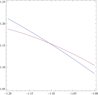
Figure 1: Contour plot of the vanishing locus of $f(v_{2},v_{3})=0$ (in blue) and $g(v_{2},v_{3})=0$ (in red), showing a common zero at $(v_{2},v_{3})=(-1.104,1.155)$.

As generally described at the beginning of this section, by turning on some of the fluxes (5.22), we can generate a potential for the axion $\theta=u^{4}$. To first order, this potential can be determined by integrating out the other moduli and setting them to their stabilized values (5.27). In general this gives a quartic effective potential for $\theta$, but choosing for instance $f_{4}\neq 0$ we get only a quadratic one

$$\begin{split}V_{\rm eff}(\theta)={M_{\rm pl}^{4}\over 4\pi{\cal V}^{2}}\,\bigl{(}f_{4}\bigr{)}^{2}\left(a+{b\over c}\hskip 1.0pt\theta^{2}\right),\end{split}$$ (5.28)

where the numerical parameters are given by $a=0.46$ and $b=0.33$. The parameter $c$ arises after canonically normalizing $\theta$, which in this example takes the numerical value $c=1.41$. Note that due to our first-order approximation, the value of the potential at the minimum $\theta=0$ is non-vanishing.

As already observed, the flux parameter $f_{4}$ does not allow to lower the mass of the inflaton to arbitrary small values. In this concrete case, for the reasonable choice ${\cal V}\sim 500$ and $f_{4}=1$, it would come out two orders of magnitude too high. Whether the parameter $b/c$ helps in this respect remains to be seen. Note that its value depends on the other fluxes and the values of the frozen moduli. Not unrelated, it also remains to stabilize the overall volume modulus ${\cal V}$ such that its mass is larger than the inflaton mass. However, these more detailed questions are beyond the scope of this paper and are postponed to a more exhaustive model search. One of the outcomes of our analysis is that now at least we know where we have to look for such models.

6 Conclusions

In this paper we have investigated whether axion monodromy inflation can be realized by the flux-induced no-scale F-term potential of type IIB orientifolds. We have chosen this framework for mainly two reasons: it provides a well-defined setting, and it allows to easily circumvent the no-go theorem of [48]. Due to the no-scale structure, the scalar potential admits also many supersymmetry breaking vacua.

From studying a simple example on the isotropic torus, we learned that fluxes can parametrically control the mass hierarchy between the light and heavy moduli, but they do not allow to control the trans-Planckian regime (of the tree-level scalar potential). In other words, a parametrically-large effective axionic $f$-parameter cannot be generated by a tuning of fluxes, at least not in the examples we were studying.

The main results of our analysis are twofold. On the one hand it is possible to keep one linear combination of complex-structure axions light, while having all other complex-structure moduli and the axio-dilaton stabilized at a higher scale. On the other hand, this is not possible when the linear combination of axions involves the universal axion $C_{0}$. In the latter case, a no-go theorem states that the light (massless) axion is always accompanied by another light (massless) combination of saxions and axions.

Our no-go theorem directly applies to the proposal of [34] (and also [18]), where the inflaton was identified with a linear combination involving the universal axion $C_{0}$, but models with additional contributions to the scalar potential might avoid this no-go theorem. These can occur through D-brane instanton effects (contributing to the non-perturbative superpotential), geometric and non-geometric fluxes (contributing to the tree-level superpotential), or perturbative corrections to the Kähler potential for the Kähler moduli which break the no-scale structure. However, including such effects makes the whole construction much more involved and less controlled.

For stabilizing all complex-structure moduli and the axio-dilaton but keeping one axionic field unconstrained, the axion has to be a linear combination of only complex-structure axions and the constraint $1<{\rm rk}(\kappa_{Nij})<h^{2,1}-1$ has to be satisfied, where $N$ is the axionic massless direction. For a concrete model we were able to show that these constraints can indeed be satisfied, and that a single axionic modulus remains massless while all other complex-structure moduli are massive. Turning on additional flux generated a mass hierarchy between the light inflaton and the heavy other moduli, where however the backreaction of the inflaton potential on the heavy moduli has been neglected.

Let us emphasize that in this paper we studied moduli stabilization only for the complex-structure moduli (in the large complex-structure limit); for realistic models one also has to satisfy additional constraints such as the tadpole cancellation conditions and one has to stabilize the Kähler moduli at mass scales larger than the axion mass. Moreover, one needs to identify a concrete Calabi-Yau manifold, compute the Kähler cone of its mirror dual and check whether the moduli are frozen self-consistently in the large complex structure regime. Clearly, it would be important to perform a similar systematic analysis also for the other proposed scenarios of F-term monodromy inflation.

Acknowledgments: We thank Alexander Westphal for useful correspondence in the initial stages of this work. We are also grateful to Timo Weigand for discussion. R.B. would like to express a special thanks to the Mainz Institute for Theoretical Physics (MITP) for its hospitality and support. E.P. is supported by the MIUR grant FIRB RBFR10QS5J.

Appendix A Conventions

In this appendix, we provide some details on the conventions employed for the examples discussed in section 4.

A.1 Conventions for toroidal models

For the toroidal examples of sections 4.1 and 4.2, we work on the orbifold $T^{6}/\mathbb{Z}_{2}\otimes\mathbb{Z}_{2}^{\prime}$, which was also studied in [46]. The closed three-forms on the toroidal ambient space invariant under the $\mathbb{Z}_{2}\times\mathbb{Z}_{2}^{\prime}$ orbifold symmetry are the following

$$\begin{split}&\alpha_{0}=dx^{1}\wedge dx^{2}\wedge dx^{3}\,,\qquad\quad\beta^{0}=dy^{1}\wedge dy^{2}\wedge dy^{3}\,,\\ &\alpha_{1}=dy^{1}\wedge dx^{2}\wedge dx^{3}\,,\qquad\quad\beta^{1}=-dx^{1}\wedge dy^{2}\wedge dy^{3}\,,\\ &\alpha_{2}=dx^{1}\wedge dy^{2}\wedge dx^{3}\,,\qquad\quad\beta^{2}=-dy^{1}\wedge dx^{2}\wedge dy^{3}\,,\\ &\alpha_{3}=dx^{1}\wedge dx^{2}\wedge dy^{3}\,,\qquad\quad\beta^{3}=-dy^{1}\wedge dy^{2}\wedge dx^{3}\,,\end{split}$$ (A.1)

which are Poincaré-dual to the obvious three-cycles on $T^{6}$. Expanding then the fluxes $H_{3}$ and $F_{3}$ in terms of these eight three-forms guarantees that $H_{3}$ and $F_{3}$ are invariant under the orientifold projection $\Omega\hskip 1.0ptR\hskip 1.0pt(-1)^{F_{L}}$.

The complex structures of each two-torus inside of $T^{6}$ are defined by $z^{i}=x^{i}+{\cal U}^{i}\,y^{i}$ (no summation over $i$), where ${\cal U}^{i}\equiv u^{i}+i\hskip 1.0ptv^{i}$ with $i=1,2,3$ are the complex-structure moduli. The resulting homogeneous coordinates $X^{\Lambda}$ and the derivatives $F_{\Lambda}=\partial_{\Lambda}F$ of the pre-potential are

$$\begin{split}\begin{array}[]{lcl@{\hspace{60pt}}lcl}X^{0}&=&1\,,\hfil\hskip 60.&F_{0}&=&-{\cal U}^{1}\,{\cal U}^{2}\,{\cal U}^{3}\,,\\ X^{1}&=&{\cal U}^{1}\,,\hfil\hskip 60.&F_{1}&=&{\cal U}^{2}\,{\cal U}^{3}\,,\\ X^{2}&=&{\cal U}^{2}\,,\hfil\hskip 60.&F_{2}&=&{\cal U}^{1}\,{\cal U}^{3}\,,\\ X^{3}&=&{\cal U}^{3}\,,\hfil\hskip 60.&F_{3}&=&{\cal U}^{1}\,{\cal U}^{2}\,,\end{array}\end{split}$$ (A.2)

where the latter originate from the prepotential

$$\begin{split}F={X^{1}X^{2}X^{3}\over X^{0}}={\cal U}^{1}{\cal U}^{2}{\cal U}^{3}\,.\end{split}$$ (A.3)

The corresponding period matrix takes the following form

$$\begin{split}{\cal N}=\scalebox{0.89}{\mbox{$\displaystyle\left(\begin{matrix}2\hskip 1.0ptu^{1}u^{2}u^{3}&-u^{2}u^{3}&-u^{1}u^{3}&-u^{1}u^{2}\\ \cdots&0&u^{3}&u^{2}\\ \cdots&\cdots&0&u^{1}\\ \cdots&\cdots&\cdots&0\end{matrix}\right)$}}+i\hskip 1.0pt\scalebox{0.89}{\mbox{$\displaystyle\left(\begin{matrix}q\hskip 1.0ptv^{1}v^{2}v^{3}&-v^{2}v^{3}{u^{1}\over v^{1}}&-v^{1}v^{3}{u^{2}\over v^{2}}&-v^{1}v^{2}{u^{3}\over v^{3}}\\ \cdots&{v^{2}v^{3}\over v^{1}}&0&0\\ \cdots&\cdots&{v^{1}v^{3}\over v^{2}}&0\\ \cdots&\cdots&\cdots&{v^{1}v^{2}\over v^{3}}\end{matrix}\right)$}},\end{split}$$ (A.4)

where the entries with the dots are determined by noting that $\mathcal{N}$ is symmetric. In (A.4) we have also defined

$$\begin{split}q=1+\left({u^{1}\over v^{1}}\right)^{2}+\left({u^{2}\over v^{2}}\right)^{2}+\left({u^{3}\over v^{3}}\right)^{2},\end{split}$$ (A.5)

and we note that $v^{i}<0$ corresponds to the physical domain of ${\rm Im}\,{\cal N}$.

A.2 Conventions for ${\rm IP}_{1,1,2,2,2}[8]$

The Calabi-Yau manifold studied in section 4.3 has a $\mathbb{Z}_{2}$ singularity, which has to be resolved. The resulting toric data for this manifold reads

$$\begin{split}\begin{array}[]{c|cccccc}&x_{1}&x_{2}&x_{3}&x_{4}&x_{5}&x_{6}\\ \hline\cr 4&1&1&1&1&0&0\\ 0&0&0&0&-2&1&1\\ \end{array}\end{split}$$ (A.6)

and the Hodge numbers are $(h^{2,1},h^{1,1})=(86,2)$. The Stanley-Reisner ideal takes the form

$${\rm SR}=\left\{x_{1}\,x_{2}\,x_{3}\,x_{4},x_{5}\,x_{6}\right\}\,.$$ (A.7)

The divisor $D=\{x_{5}=0\}$ is a K3 surface, and together with the divisor $H=\{x_{1}=0\}$ the intersection form becomes

$$\begin{split}I_{3}=8\,H^{3}+4\,H^{2}\,D\,.\end{split}$$ (A.8)

Performing a change of basis to $D_{1}=D$ and $D_{2}=3H-2D$, the intersection form takes the simple form $I_{3}=36\,D_{1}(D_{2})^{2}$.

For the prepotential of the mirror manifold in the large complex-structure limit we then find

$$\begin{split}F=\frac{X^{1}(X^{2})^{2}}{X^{0}}\,,\end{split}$$ (A.9)

where for convenience we have set the prefactor to one. Due to the large complex-structure limit we are considering, the complex coordinates $X^{\Lambda}$ are identical to those in (A.2), from which we can compute $F_{\Lambda}$ as

$$\begin{split}F_{0}=-{\cal U}^{1}({\cal U}^{2})^{2}\,,\qquad F_{1}=({\cal U}^{2})^{2}\,,\qquad F_{2}=2\,{\cal U}^{1}\,{\cal U}^{2}\,.\end{split}$$ (A.10)

With $q^{\prime}=\frac{(v^{2})^{2}}{v^{1}}$ the period matrix is then determined as

$$\begin{split}{\cal N}=\scalebox{0.86}{\mbox{$\displaystyle\left(\begin{matrix}2\hskip 1.0ptu^{1}(u^{2})^{2}&-(u^{2})^{2}&-2u^{1}u^{2}\\ \cdots&0&2\hskip 1.0ptu^{2}\\ \cdots&\cdots&2\hskip 1.0ptu^{1}\end{matrix}\right)$}}+i\hskip 1.0pt\scalebox{0.89}{\mbox{$\displaystyle\left(\begin{matrix}2\hskip 1.0pt(u^{2})^{2}v^{1}+(u^{1})^{2}\hskip 1.0ptq^{\prime}+v^{1}(v^{2})^{2}&-u^{1}\hskip 1.0ptq^{\prime}&-2\hskip 1.0ptu^{2}v^{1}\\ \cdots&q^{\prime}&0\\ \cdots&\cdots&2\hskip 1.0ptv^{1}\end{matrix}\right)$}}\,.\end{split}$$ (A.11)

Appendix B Proof of no-go for case B and rk(A)=N-1

In case the matrix ${\cal A}_{ij}=\kappa_{Nij}$ has rank $N-1$, its kernel is one-dimensional, and so the constraints in the second line of (5.18) are solved by $\overline{f}^{i}=a^{i}\hskip 1.0pt\overline{f}$ and $\overline{h}^{i}=a^{i}\hskip 1.0pt\overline{h}$ for the null-vector $a^{i}$. Recalling then equations (5.19), we can form linear combinations

$$\begin{split}s\hskip 1.0pt\overline{h}\hskip 1.0pt{\cal Q}_{i}+(\overline{f}+c\hskip 1.0pt\overline{h})\hskip 1.0pt{\cal P}_{i}=0\,,\end{split}$$ (B.1)

for each $i=\{1,\ldots,N\}$. Writing out (B.1), we obtain the following conditions

$$\begin{split}0=\kappa_{ijk}\hskip 1.0ptu^{j}a^{k}\Big{[}(\overline{f}+c\overline{h})^{2}+s^{2}\overline{h}^{2}\Big{]}+\Big{[}(f_{i}+ch_{i})(\overline{f}+c\overline{h})+s^{2}h_{i}\,\overline{h}\Big{]}\,,\end{split}$$ (B.2)

which do not depend on the saxions $v^{i}$ and which are trivially satisfied for $i=N$. Let us now make one technical assumption: we require that the matrix $\mathcal{B}_{\mu\nu}$ defined as

$$\begin{split}\hskip 40.0pt{\cal B}_{\mu\nu}=\kappa_{\mu\nu k}a^{k}\,,\hskip 50.0pt\mu,\nu\in\{1,\ldots,N-1\}\,,\end{split}$$ (B.3)

is regular. We can then solve (B.2) for the $N-1$ axions $u^{\mu}$ as follows

$$\begin{split}u^{\mu}=-\big{(}{\cal B}^{-1}\big{)}^{\mu\nu}\,\frac{(f_{\nu}+c\hskip 1.0pth_{\nu})\bigl{(}\overline{f}+c\hskip 1.0pt\overline{h}\bigr{)}+s^{2}h_{\nu}\hskip 1.0pt\overline{h}}{\bigl{(}\overline{f}+c\overline{h}\bigr{)}^{2}+s^{2}\overline{h}^{2}}\,.\end{split}$$ (B.4)

Let us also consider the following linear combinations

$$\begin{split}\begin{array}[]{lll}{\cal P}_{0}+{\cal P}_{i}\hskip 1.0ptu^{i}&=f_{0}+f_{\mu}\hskip 1.0ptu^{\mu}+{\cal B}_{\mu\nu}u^{\mu}u^{\nu}\hskip 1.0pt\overline{f}&=0\,,\\[5.0pt] {\cal Q}_{0}+{\cal Q}_{i}\hskip 1.0ptu^{i}&=h_{0}+h_{\mu}\hskip 1.0ptu^{\mu}+{\cal B}_{\mu\nu}u^{\mu}u^{\nu}\hskip 1.0pt\overline{h}&=0\,,\end{array}\end{split}$$ (B.5)

which we can combine into

$$0 =\bigl{(}h_{0}\hskip 1.0pt\overline{f}-f_{0}\hskip 1.0pt\overline{h}\bigr{)}+\bigl{(}h_{\mu}\overline{f}-f_{\mu}\overline{h}\bigr{)}u^{\mu}\,,$$ (B.6)

$$0 =h_{0}+h_{\mu}\hskip 1.0ptu^{\mu}+{\cal B}_{\mu\nu}u^{\mu}u^{\nu}\hskip 1.0pt\overline{h}\,.$$ (B.7)

Let us note that (B.4) together with (B.6) and (B.7) provide $N+1$ equations for the $N+1$ fields $\{u^{1},\ldots,u^{N-1},c,s\}$. To proceed, we define the following quantities which do not depend on any of the moduli

$$\begin{split}\mathsf{H}=h_{\mu}\hskip 1.0pt\big{(}{\cal B}^{-1}\big{)}^{\mu\nu}\hskip 1.0pth_{\nu}\,,\hskip 40.0pt\mathsf{G}=h_{\mu}\hskip 1.0pt\big{(}{\cal B}^{-1}\big{)}^{\mu\nu}\hskip 1.0ptf_{\nu}\,,\hskip 40.0pt\mathsf{F}=f_{\mu}\hskip 1.0pt\big{(}{\cal B}^{-1}\big{)}^{\mu\nu}\hskip 1.0ptf_{\nu}\,.\end{split}$$ (B.8)

Employing (B.4) then in (B.6) we find

$$\begin{split}s^{2}=\bigl{(}\overline{f}+c\hskip 1.0pt\overline{h}\bigr{)}\,\frac{\overline{f}\hskip 1.0pt(\mathsf{G}+c\hskip 1.0pt\mathsf{H})-\overline{h}\hskip 1.0pt(\mathsf{F}+c\hskip 1.0pt\mathsf{H})-\big{(}\overline{f}+c\hskip 1.0pt\overline{h}\bigr{)}\bigl{(}h_{0}\hskip 1.0pt\overline{f}-f_{0}\hskip 1.0pt\overline{h}\bigr{)}}{\bigl{(}h_{0}\hskip 1.0pt\overline{f}-f_{0}\hskip 1.0pt\overline{h}\bigr{)}\hskip 1.0pt\overline{h}^{2}-\overline{h}\hskip 1.0pt\overline{f}\hskip 1.0pt\mathsf{H}+\overline{h}^{2}\hskip 1.0pt\mathsf{G}}\,,\end{split}$$ (B.9)

and for (B.4) in (B.7) we obtain an expression which only depends on $s^{2}$. Using then furthermore (B.9) we arrive at

$$\begin{split}0=\overline{h}\,\frac{\bigl{(}h_{0}\hskip 1.0pt\overline{f}-f_{0}\hskip 1.0pt\overline{h}\bigr{)}^{2}+2\hskip 1.0pth_{0}\bigl{(}\overline{h}\hskip 1.0pt\mathsf{F}-\overline{f}\hskip 1.0pt\mathsf{G}\bigr{)}+2\hskip 1.0ptf_{0}\bigl{(}\overline{f}\hskip 1.0pt\mathsf{H}-\overline{h}\hskip 1.0pt\mathsf{G}\bigr{)}+\mathsf{G}^{2}-\mathsf{F}\hskip 1.0pt\mathsf{H}}{\overline{f}^{2}\mathsf{H}+\overline{h}^{2}\hskip 1.0pt\mathsf{F}-2\hskip 1.0pt\overline{f}\hskip 1.0pt\overline{h}\hskip 1.0pt\mathsf{G}}\,,\end{split}$$ (B.10)

which is a relation only on the fluxes and does not depend on any moduli. We therefore have $N$ equations for the $N+1$ moduli $\{u^{1},\ldots,u^{N-1},c,s\}$, implying that one modulus is always unfixed.

References

- [1] BICEP2 Collaboration Collaboration, P. Ade et al., “Detection of B-Mode Polarization at Degree Angular Scales by BICEP2,” Phys.Rev.Lett. 112 (2014) 241101, 1403.3985.
- [2] Planck Collaboration Collaboration, R. Adam et al., “Planck intermediate results. XXX. The angular power spectrum of polarized dust emission at intermediate and high Galactic latitudes,” 1409.5738.
- [3] C. Burgess, M. Cicoli, and F. Quevedo, “String Inflation After Planck 2013,” JCAP 1311 (2013) 003, 1306.3512.
- [4] E. Silverstein, “Les Houches lectures on inflationary observables and string theory,” 1311.2312.
- [5] D. Baumann and L. McAllister, “Inflation and String Theory,” 1404.2601.
- [6] D. H. Lyth, “What would we learn by detecting a gravitational wave signal in the cosmic microwave background anisotropy?,” Phys.Rev.Lett. 78 (1997) 1861–1863, hep-ph/9606387.
- [7] L. McAllister, E. Silverstein, A. Westphal, and T. Wrase, “The Powers of Monodromy,” 1405.3652.
- [8] A. Hebecker, S. C. Kraus, and L. T. Witkowski, “D7-Brane Chaotic Inflation,” Phys.Lett. B737 (2014) 16–22, 1404.3711.
- [9] L. E. Ibanez and I. Valenzuela, “The Inflaton as a MSSM Higgs and Open String Modulus Monodromy Inflation,” 1404.5235.
- [10] K. Freese, J. A. Frieman, and A. V. Olinto, “Natural inflation with pseudo - Nambu-Goldstone bosons,” Phys.Rev.Lett. 65 (1990) 3233–3236.
- [11] F. C. Adams, J. R. Bond, K. Freese, J. A. Frieman, and A. V. Olinto, “Natural inflation: Particle physics models, power law spectra for large scale structure, and constraints from COBE,” Phys.Rev. D47 (1993) 426–455, hep-ph/9207245.
- [12] P. Svrcek and E. Witten, “Axions In String Theory,” JHEP 0606 (2006) 051, hep-th/0605206.
- [13] T. W. Grimm, “Axion Inflation in F-theory,” 1404.4268.
- [14] J. E. Kim, H. P. Nilles, and M. Peloso, “Completing natural inflation,” JCAP 0501 (2005) 005, hep-ph/0409138.
- [15] R. Kappl, S. Krippendorf, and H. P. Nilles, “Aligned Natural Inflation: Monodromies of two Axions,” Phys.Lett. B737 (2014) 124–128, 1404.7127.
- [16] I. Ben-Dayan, F. G. Pedro, and A. Westphal, “Hierarchical Axion Inflation,” 1404.7773.
- [17] C. Long, L. McAllister, and P. McGuirk, “Aligned Natural Inflation in String Theory,” Phys.Rev. D90 (2014) 023501, 1404.7852.
- [18] X. Gao, T. Li, and P. Shukla, “Combining Universal and Odd RR Axions for Aligned Natural Inflation,” 1406.0341.
- [19] S. Dimopoulos, S. Kachru, J. McGreevy, and J. G. Wacker, “N-flation,” JCAP 0808 (2008) 003, hep-th/0507205.
- [20] T. W. Grimm, “Axion inflation in type II string theory,” Phys.Rev. D77 (2008) 126007, 0710.3883.
- [21] M. Cicoli, K. Dutta, and A. Maharana, “N-flation with Hierarchically Light Axions in String Compactifications,” JCAP 1408 (2014) 012, 1401.2579.
- [22] T. C. Bachlechner, M. Dias, J. Frazer, and L. McAllister, “A New Angle on Chaotic Inflation,” 1404.7496.
- [23] A. R. Liddle, A. Mazumdar, and F. E. Schunck, “Assisted inflation,” Phys.Rev. D58 (1998) 061301, astro-ph/9804177.
- [24] A. Ashoorioon, H. Firouzjahi, and M. Sheikh-Jabbari, “M-flation: Inflation From Matrix Valued Scalar Fields,” JCAP 0906 (2009) 018, 0903.1481.
- [25] A. Ashoorioon and M. Sheikh-Jabbari, “Gauged M-flation, its UV sensitivity and Spectator Species,” JCAP 1106 (2011) 014, 1101.0048.
- [26] E. Silverstein and A. Westphal, “Monodromy in the CMB: Gravity Waves and String Inflation,” Phys.Rev. D78 (2008) 106003, 0803.3085.
- [27] L. McAllister, E. Silverstein, and A. Westphal, “Gravity Waves and Linear Inflation from Axion Monodromy,” Phys.Rev. D82 (2010) 046003, 0808.0706.
- [28] N. Kaloper and L. Sorbo, “A Natural Framework for Chaotic Inflation,” Phys.Rev.Lett. 102 (2009) 121301, 0811.1989.
- [29] N. Kaloper, A. Lawrence, and L. Sorbo, “An Ignoble Approach to Large Field Inflation,” JCAP 1103 (2011) 023, 1101.0026.
- [30] A. Westphal, “String Cosmology - Large-Field Inflation in String Theory,” 1409.5350.
- [31] E. Palti and T. Weigand, “Towards large r from [p, q]-inflation,” JHEP 1404 (2014) 155, 1403.7507.
- [32] J. P. Conlon, “Brane-Antibrane Backreaction in Axion Monodromy Inflation,” JCAP 1201 (2012) 033, 1110.6454.
- [33] F. Marchesano, G. Shiu, and A. M. Uranga, “F-term Axion Monodromy Inflation,” 1404.3040.
- [34] R. Blumenhagen and E. Plauschinn, “Towards Universal Axion Inflation and Reheating in String Theory,” Phys.Lett. B736 (2014) 482–487, 1404.3542.
- [35] M. Arends, A. Hebecker, K. Heimpel, S. C. Kraus, D. Lust, et al., “D7-Brane Moduli Space in Axion Monodromy and Fluxbrane Inflation,” Fortsch.Phys. 62 (2014) 647–702, 1405.0283.
- [36] S. Franco, D. Galloni, A. Retolaza, and A. Uranga, “Axion Monodromy Inflation on Warped Throats,” 1405.7044.
- [37] F. Hassler, D. Lüst, and S. Massai, “On Inflation and de Sitter in Non-Geometric String Backgrounds,” 1405.2325.
- [38] Z. Kenton and S. Thomas, “D-brane Potentials in the Warped Resolved Conifold and Natural Inflation,” 1409.1221.
- [39] X. Gao, T. Li, and P. Shukla, “Fractional chaotic inflation in the lights of PLANCK and BICEP2,” 1404.5230.
- [40] S. Kachru, R. Kallosh, A. D. Linde, and S. P. Trivedi, “De Sitter vacua in string theory,” Phys.Rev. D68 (2003) 046005, hep-th/0301240.
- [41] V. Balasubramanian, P. Berglund, J. P. Conlon, and F. Quevedo, “Systematics of moduli stabilisation in Calabi-Yau flux compactifications,” JHEP 0503 (2005) 007, hep-th/0502058.
- [42] T. R. Taylor and C. Vafa, “R R flux on Calabi-Yau and partial supersymmetry breaking,” Phys.Lett. B474 (2000) 130–137, hep-th/9912152.
- [43] S. B. Giddings, S. Kachru, and J. Polchinski, “Hierarchies from fluxes in string compactifications,” Phys.Rev. D66 (2002) 106006, hep-th/0105097.
- [44] S. Gukov, C. Vafa, and E. Witten, “CFT’s from Calabi-Yau four folds,” Nucl.Phys. B584 (2000) 69–108, hep-th/9906070.
- [45] S. Hosono, A. Klemm, and S. Theisen, “Lectures on mirror symmetry,” Lect.Notes Phys. 436 (1994) 235, hep-th/9403096.
- [46] R. Blumenhagen, D. Lüst, and T. R. Taylor, “Moduli stabilization in chiral type IIB orientifold models with fluxes,” Nucl.Phys. B663 (2003) 319–342, hep-th/0303016.
- [47] A. A. Starobinsky, “A New Type of Isotropic Cosmological Models Without Singularity,” Phys.Lett. B91 (1980) 99–102.
- [48] J. P. Conlon, “The QCD axion and moduli stabilisation,” JHEP 0605 (2006) 078, hep-th/0602233.