Symplectic and Semiclassical Aspects of the Schläfli Identity

Abstract

The Schläfli identity, which is important in Regge calculus and loop quantum gravity, is examined from a symplectic and semiclassical standpoint in the special case of flat, 3-dimensional space. In this case a proof is given, based on symplectic geometry. A series of symplectic and Lagrangian manifolds related to the Schläfli identity, including several versions of a Lagrangian manifold of tetrahedra, are discussed. Semiclassical interpretations of the various steps are provided. Possible generalizations to 3-dimensional spaces of constant (nonzero) curvature, involving Poisson-Lie groups and $q$-deformed spin networks, are discussed.

1 Introduction

The Schläfli identity, which is familiar in applications of Regge calculus in general relativity (Regge 1961; Misner, Thorne and Wheeler 1973; Regge and Williams 2000), is a differential relation connecting the volume of a polyhedron in an $n$-dimensional space of constant curvature with the $(n-2)$-volumes and dihedral angles of its $(n-2)$-dimensional faces. In this article we deal with the special case of a tetrahedron in Euclidean ${\mathbb{R}}^{3}$, for which the identity itself is given by (4) below. In this case we provide an apparently new proof of the Schläfli identity, one based on symplectic geometry. We also discuss some geometrical constructions related to the proof, including a pair of symplectic reductions that take us from a 48-dimensional symplectic manifold in which the proof is set to a 12-dimensional symplectic manifold in which the space of tetrahedra is realized as a Lagrangian submanifold. The inspiration for our proof comes from a semiclassical or asymptotic analysis of the Wigner $6j$-symbol (Wigner 1959, Edmonds 1960, Ponzano and Regge 1968, Schulten and Gordon 1975ab, Biedenharn and Louck 1981, Roberts 1999, Taylor and Woodward 2005, Aquilanti et al2012). As our analysis proceeds we provide semiclassical interpretations of many of the steps.

The Schläfli identity is useful for obtaining formulas for the volume of polyhedra in spaces of constant curvature. Schläfli’s (1858) original derivation concerned spaces of positive curvature (we note that several of the citations to this article in the recent literature are incorrect). The result was generalized to spaces of negative curvature by Sforza (1907) and new proofs given by Kneser (1936). More recent treatments include Milnor (1994), Alekseevskij, Vinberg and Solodovnikov (1993) and Yakut, Savas and Kader (2009).

Another approach to the Schl afli identity has been explored recently (Rivin and Schlenker 2000, Souam 2004). It begins with a formula which is valid for an arbitrary hypersurface embedded in an Einstein manifold (a manifold of constant curvature whose metric satisfies the Einstein equations with a cosmological constant). The formula relates the variation of the volume enclosed by the hypersurface to variations of the extrinsic curvature and induced metric on the hypersurface. We have shown that the same formula can be obtained by varying the Einstein-Hilbert action (the integral of the curvature scalar) evaluated on the enclosed region and relating that variation to a surface integral over the boundary using manipulations similar to those employed in the ADM formalism in general relativity (Misner, Thorne and Wheeler 1973, Thiemann 2007). For a polyhedron, the extrinsic curvature is concentrated in the manner of a delta function on the codimension two faces of the polyhedron, where its integral is related to the dihedral angles. When applied to the polyhedron, the formula thus reduces to the Schläfli identity.

Although our (symplectic) proof of the Schläfli identity stands on its own, the applications that we have in mind are related to Regge calculus, an approach to discretizing general relativity, and to loop quantum gravity, which also involves a discretization of the degrees of freedom of the gravitational field. See, for example, Barrett and Steele (2003), Livine and Oriti (2003), Dittrich, Freidel and Speziale (2007), and Bahr and Dittrich (2009, 2010), where the Schläfli identity plays a crucial role. See also Carfora and Marzuoli (2012) for a modern, comprehensive review of simplicial methods in quantum gravity and other fields, including the role of state sums and their regularizations. We suspect that our symplectic approach to the Schläfli identity may be especially relevant in loop quantum gravity, where spin networks such as the $6j$-symbol play an important role and where the classical phase space (Freidel and Speziale 2010, Livine and Tambornino 2011) has been identified with the same symplectic manifolds that appear in our analysis.

We begin in Sec. 2 by explaining the shape space of tetrahedra and by presenting an ad hoc construction of a symplectic manifold and a submanifold thereof that can be identified with the space of tetrahedra. This submanifold is Lagrangian by virtue of the Schläfli identity, with a generating function (7) that we call the “Ponzano-Regge phase.” In Sec. 3 we present an integral representation of the Ponzano-Regge phase, essentially a derivation of the phase of the asymptotic expression for the Wigner $6j$-symbol, following the method of Roberts (1999). In Sec. 4 we present a proof of the Schläfli identity using this integral representation. The method of proof involves integrating the symplectic form over a certain surface in phase space and then using Stokes’ theorem, in a manner common to several basic proofs in classical mechanics (Arnold 1989). Then in Secs. 5 and 6 we carry out a sequence of two symplectic reductions on the symplectic manifold in which the proof of the Schläfli identity is set, recovering at the end the symplectic manifold and Lagrangian submanifold of tetrahedra that we started with in Sec. 2. In Sec. 7 we present various remarks and conclusions, including a outline of some of the features of the generalization of this work to the $q$-deformed $6j$-symbol and the Schläfli identity in spaces of constant, nonzero curvature.

2 The Shape Space and Lagrangian Manifold of Tetrahedra

2.1 Tetrahedra and Their Shapes

A tetrahedron may be defined as a subset of Euclidean ${\mathbb{R}}^{3}$ in terms of an ordered set of four points, which are the vertices. The six edges and their lengths are defined in terms of the vertices. As special cases we allow the tetrahedron to be flat (the four vertices may lie in a plane) or of lower dimensionality (the vertices may lie in a line or they may all coincide). Any or all of the vertices are allowed to coincide, so that some or all of the edge lengths may be zero.

By this definition the space of tetrahedra is $({\mathbb{R}}^{3})^{4}$. If we consider two tetrahedra equivalent that are related by translations, then the space reduces to $({\mathbb{R}}^{3})^{3}$, in which the three vectors can be taken as the edge vectors emanating from a given vertex. If we expand the equivalence classes to include proper rotations, then the space of tetrahedra reduces to what we will call the “shape space of tetrahedra,”

$${\cal S}=\frac{({\mathbb{R}}^{3})^{3}}{SO(3)}\cong{\mathbb{R}}^{6},$$ (1)

where the action of $SO(3)$ is the diagonal action on all three copies of ${\mathbb{R}}^{3}$ (that is, it is a rigid, proper rotation of the tetrahedron) and where $\cong$ means “is diffeomorphic to.” This is shown by Narasimhan and Ramadas (1979) and discussed further by Littlejohn and Reinsch (1995). In the following two tetrahedra will be considered to have the same shape if they are related by a translation and a proper rotation.

Then it turns out that the space of flat tetrahedra (those whose vertices lie in a plane in ${\mathbb{R}}^{3}$) constitute a subspace ${\mathbb{R}}^{5}\subset{\cal S}\cong{\mathbb{R}}^{6}$, which we will call the “shape space of flat tetrahedra.” If we define the volume $V$ of the tetrahedron as $1/6$ the triple product of three vectors emanating from a given vertex, then the subspace ${\mathbb{R}}^{5}$ of flat tetrahedra divides shape space ${\cal S}$ into three subsets, those on which $V>0$, $V<0$ and $V=0$ (the last being the subspace ${\mathbb{R}}^{5}$ of flat tetrahedra itself). Furthermore, performing a spatial inversion of a tetrahedron in ${\mathbb{R}}^{3}$ causes the point of ${\cal S}$ to be reflected in the hyperplane ${\mathbb{R}}^{5}$ of flat tetrahedra. In particular, the shape of a tetrahedron is invariant under spatial inversion if and only if it is flat.

It is also shown in the references cited that the six edge lengths of the tetrahedron form a coordinate system on the regions $V\geq 0$ and $V\leq 0$ of ${\cal S}$, that is, there is a one-to-one map from these regions of ${\cal S}$ to a region of the six dimensional space with coordinates $J_{r}$, $r=1,\ldots,6$, where $J_{r}$ is the length of edge $r$. This map is not onto, however, since there are values of the $J_{r}$ that do not correspond to any tetrahedron. In the first place these lengths obviously must satisfy $J_{r}\geq 0$ and the four triangle inequalities for the four faces of the tetrahedron; in addition, there is a further requirement that the faces can be assembled into a tetrahedron. All these conditions can be expressed in terms of the minors of the Cayley-Menger determinant (Ponzano and Regge 1968) or of an associated Gram matrix (Littlejohn and Yu 2009). Spatial inversion maps a tetrahedron with volume $V$ into one with volume $-V$, without changing the edge lengths $J_{r}$; therefore, given edge lengths such that a tetrahedron exists, the shape of the tetrahedron is determined to within a spatial inversion (hence uniquely, for a flat tetrahedron).

We now define the dihedral angle $\psi_{r}$ associated with edge $r$ for a tetrahedron of a given shape, first for the case $V\geq 0$. A given edge is the intersection of two adjacent faces; the dihedral angle is not defined unless the areas of the two faces are nonzero, so we assume this. (If a face has zero area, then we will refer to it as “degenerate.”) Then we define the dihedral angle $\psi_{r}$ as the angle between the outward pointing normals to the two faces. This gives $0\leq\psi_{r}\leq\pi$. Finally, if $V<0$, we define $\psi_{r}$ as the negative of the angle $\psi_{r}$ for the spatially inverted shape (which has $V>0$). With these conventions, the dihedral angles lie in the range $-\pi<\psi_{r}\leq\pi$, and all dihedral angles change sign under spatial inversion, modulo $2\pi$.

The subset of shape space on which one or more dihedral angles are not defined consists of tetrahedra with one or more degenerate faces. All such tetrahedra have zero volume, so they form a subset of the shape space ${\mathbb{R}}^{5}$ of flat tetrahedra. This subset has codimension 1 inside ${\mathbb{R}}^{5}$ (more precisely, it is the union of smooth manifolds, of which the maximum dimensionality is 4). If the dihedral angles $\psi_{r}$ are defined for a flat tetrahedron, then they are either 0 or $\pi$, and are constant inside connected regions of the space ${\mathbb{R}}^{5}$ of flat tetrahedra; these regions are separated by the codimension 1 subset upon which some face is degenerate. We will denote the subset of shape space ${\cal S}$ upon which the dihedral angles are defined by ${\dot{\cal S}}$; it is ${\cal S}$ minus the tetrahedra with one or more degenerate faces.

Our definition of the dihedral angles differs from the usual one used in discussions of the Schläfli identity, which is the absolute value of the definition given here. Our definition has the advantage that the dihedral angles are smooth functions along a smooth curve crossing the subspace ${\mathbb{R}}^{5}$ of flat tetrahedra, modulo $2\pi$, if we avoid shapes with degenerate faces. More precisely, all dihedral angles are either 0 or $\pi$ on the subspace ${\mathbb{R}}^{5}$ of flat tetrahedra, as long as we avoid degenerate faces; as we pass from the region $V>0$ to the region $V<0$ through this subspace, an angle which is 0 on the flat tetrahedron passes smoothly from positive to negative values, while an angle that is $\pi$ on the flat tetrahedron jumps discontinuously from $+\pi$ to $-\pi$. In both cases, the differential $d\psi_{r}$ is smooth. As an example of such a motion we may rotate two adjacent faces relative to one another about their common edge, so that one face passes through the plane of the other. Along this motion the lengths of all the edges are constant except for the one opposite the edge common to the two faces.

We remark that the inclusion of negative angles in the definition of the dihedral angles is merely a convenience in the case of the asymptotics of the $6j$-symbol, but such an extension to a full range of $2\pi$ in the dihedral angles is necessary for more complex spin networks, such as the $9j$-symbol. The definition of dihedral angles given here is equivalent to the general definition given by Haggard and Littlejohn (2010). In addition, negative dihedral angles emerge naturally at the end of the sequence of symplectic reductions carried out in this paper (see Sec. 6).

If a tetrahedron has one or more edge lengths that are zero (that is, if two or more vertices coincide), then two or more faces are degenerate; these tetrahedra form a set of shapes that is a subset of the tetrahedra with degenerate faces. It has codimension 2 inside the space ${\mathbb{R}}^{5}$ of flat tetrahedra.

2.2 Lagrangian Interpretation of the Schläfli Identity

For the time being we concentrate on the region $V>0$, where the dihedral angles $\psi_{r}$ are functions of the edge lengths $J_{r}$. Since the $\psi_{r}$ do not change if the edge lengths are scaled by some positive factor, Euler’s theorem on homogeneous functions implies

$$\sum_{r}J_{r}\frac{\partial\psi_{s}}{\partial J_{r}}=0.$$ (2)

The Schläfli identity has a similar appearance; it is

$$\sum_{r}J_{r}\frac{\partial\psi_{r}}{\partial J_{s}}=0,$$ (3)

which, after multiplying by $dJ_{s}$ and summing over $s$, can be written

$$\sum_{r}J_{r}\,d\psi_{r}=0.$$ (4)

See Luo (2008) for other identities involving the matrix $\partial\psi_{r}/\partial J_{s}$, including the case of tetrahedra in spaces of constant (nonzero) curvature.

If we differentiate (3) with respect to $J_{k}$ and antisymmetrize in $k$ and $s$, we obtain

$$\frac{\partial\psi_{k}}{\partial J_{s}}=\frac{\partial\psi_{s}}{\partial J_{k}},$$ (5)

that is, the matrix $\partial\psi_{k}/\partial J_{s}$ is symmetric. Thus the Schläfli identity (3) implies the Euler identity (2). It also implies

$$\psi_{r}=\frac{\partial S}{\partial J_{r}},$$ (6)

where $S$ is given by

$$S=\sum_{r}J_{r}\,\psi_{r}.$$ (7)

We refer to $S$ as the “Ponzano-Regge phase” since it appears in the factor $\cos(S+\pi/4)$ in the asymptotic formula for the Wigner $6j$-symbol due to Ponzano and Regge (1968).

Figure 1: The tetrahedra form a Lagrangian manifold in the 12-dimensional space with coordinates $J_{r}$ and $\psi_{r}$, $r=1,\ldots,6$.

These relations imply that the space of tetrahedra is a Lagrangian submanifold of a 12-dimensional space with coordinates $(J_{1},\ldots,J_{6},\psi_{1},\ldots,\psi_{6})$, of which a schematic illustration is given in Fig. 1. The 6-dimensional manifold $L$ is the graph of the functions (6); because it is the graph of a gradient, $L$ is Lagrangian with respect to the symplectic form,

$$\sum_{r}dJ_{r}\wedge d\psi_{r}=d\sum_{r}J_{r}\,d\psi_{r}.$$ (8)

The figure shows a point $x$ of the 6-dimensional space of edge lengths (call it “$J$-space”) and the vertical manifold of constant edge lengths above it which intersects $L$ in the point $y$, which in turn projects onto the space of angles (call it “$\psi$-space”) at point $a$. Due to the homogeneity of the functions $\psi_{r}(J_{1},\ldots,J_{6})$, the point $a$ does not move if $x$ is moved along the radial line $R$ in $J$-space, that is, if the edge lengths are scaled by a common factor. This means that the line $a$–$y$ is everywhere tangent to $L$, and that $L$ is vertical in one dimension over $\psi$-space. Manifold $L$, which is 6-dimensional and which has a nonsingular projection onto $J$-space, has only a 5-dimensional projection onto $\psi$-space. That is, points of $\psi$-space that can be realized as dihedral angles of a tetrahedron are first order caustic points of the projection from $L$.

The construction given has applied in the region $V>0$. The same construction works in the region $V<0$, providing a second branch to the manifold illustrated in Fig. 1, obtained from the first by $\psi_{r}\mapsto-\psi_{r}$. On the subset $V=0$, excluding shapes with degenerate faces, the main problem is the angles $\psi_{r}$ that jump discontinuously from $\pi$ to $-\pi$. We can avoid this by speaking of a trivial $T^{6}$-bundle over ${\dot{\cal S}}$. Then what we are calling the functions $\psi_{r}(J_{1},\ldots,J_{6})$ becomes a smooth section of this bundle, that is, the surface $L$, extended to flat shapes with nondegenerate faces. Then the differential forms $d\psi_{r}$ and the combination seen in (4) are well defined everywhere in the bundle, and the Schläfli identity in the form (4) holds everywhere on $L$. Also, the Ponzano-Regge phase $S$, which involves the angles $\psi_{r}$ themselves (not their differentials), is a function on $L$; but it is discontinuous at the flat shapes.

In our next step we exploit a certain integral representation for the Ponzano-Regge phase $S$. It turns out that $S$ can be expressed as a line integral of a symplectic 1-form in a certain 48-dimensional symplectic manifold along a path running along one 24-dimensional Lagrangian submanifold and then back along another, in the type of geometry that arises in the semiclassical analysis of scalar products $\langle A|B\rangle$ in quantum mechanics. This is explained in Sec. 3. This representation is then used in Sec. 4 to prove the Schläfli identity. Then in subsequent sections it is shown that the 12-dimensional symplectic manifold illustrated in Fig. 1 (“$J$–$\psi$-space” or the $T^{6}$ bundle just described) can be obtained from the 48-dimensional one in which the integral representation is expressed by means of two symplectic reductions. This process reveals information about the symplectic manifold in Fig. 1 that is not apparent from the presentation so far.

3 An Integral Representation of the Ponzano-Regge Phase

In this section we present a derivation of the Ponzano-Regge phase as the principal contribution to the phase of the asymptotic expression for the Wigner $6j$-symbol. The derivation is a reformulation of that given by Roberts (1999), which as far as we know is the most symmetrical and elegant available. We express it, however, in a somewhat different geometrical language than Roberts, using real Lagrangian manifolds that are parameterized as level sets of various momentum maps and an arbitrary real representation of the wave functions, rather than a complex or coherent state representation. We invoke the semiclassical treatment of the $6j$-symbol merely to motivate the geometry behind the representation of the Ponzano-Regge phase as a certain line integral along certain Lagrangian manifolds; this is what we will need for our proof of the Schläfli identity in Sec. 4. For the purposes of this paper the manifolds need not be quantized.

Our brief discussion of the semiclassical mechanics of the $6j$-symbol involves what we call the “$12j$-model” of the $6j$-symbol, which is due to Roberts (1999) and which is explained in terms of spin networks in Sec. 3 of Aquilanti et al(2012). In this model, the $6j$-symbol is expressed as the scalar product $\langle A|B\rangle$ of two vectors $|A\rangle$ and $|B\rangle$ in a certain Hilbert space, where the labels $A$ and $B$ stand for two complete sets of commuting observables of which the vectors are eigenvectors, with certain normalization and phase conventions. The two complete sets involve angular momentum operators whose components do not commute except on the subspace where the angular momenta vanish, which is precisely the subspace in terms of which the $6j$-symbol is defined. These two sets of commuting operators correspond classically to two sets of Poisson commuting functions on a certain phase space. Again, the sets involve various (now classical) angular momenta whose components do not Poisson commute except on the level set upon which the angular momenta vanish, which are precisely the Lagrangian manifolds relevant to the semiclassical evaluation of the scalar product $\langle A|B\rangle$.

3.1 Phase spaces

We now explain the phase space in which these manifolds live. The notation is the same as in Aquilanti et al(2007, 2012), with minor modifications which are noted. We begin with the phase space or symplectic manifold $\Phi$ of a 2-dimensional, isotropic harmonic oscillator with unit mass and frequency. This is a classical version of the harmonic oscillator system used by Schwinger (1952) and Bargmann (1962) in their treatment of the representation theory of $SU(2)$, which anticipated many of the features of the modern theory of geometric quantization (Kirillov 1976, Simms and Woodhouse 1977, Bates and Weinstein 1997, Echeverría-Enríquez et al1999). Coordinates on $\Phi$ are $(x_{1},x_{2},p_{1},p_{2})$, so that as a symplectic manifold $\Phi=({\mathbb{R}}^{4},dp\wedge dx)$, where $dp\wedge dx$ means $\sum_{\mu}dp_{\mu}\wedge dx_{\mu}$. We use indices $\mu$, $\nu$, etc to run over 1,2, indexing the two harmonic oscillators; we often suppress these indices with an implied summation. We introduce complex coordinates $z_{\mu}=(x_{\mu}+ip_{\mu})/\sqrt{2}$, ${\bar{z}}_{\mu}=(x_{\mu}-ip_{\mu})/\sqrt{2}$ on $\Phi$, so that $\Phi$ can be seen as $({\mathbb{C}}^{2},idz^{\dagger}\wedge dz)$, where $z$ (without the $\mu$ subscript) is seen as a column vector or spinor $(z_{1},z_{2})^{T}$, where $z^{\dagger}$ is seen as a row spinor $({\bar{z}}_{1},{\bar{z}}_{2})$ and where again a summation over $\mu$ is implied. We denote the symplectic 2-form on $\Phi$ by $\omega=d\theta$, where $\theta$ can be taken to be $iz^{\dagger}\,dz$. Although $\theta$ is complex, we will be only interested in integrals of it along closed loops, for which the integrals are real.

The phase space $\Phi$ has several functions defined on it, including

$$I=\frac{1}{2}z^{\dagger}z,\qquad J_{i}=\frac{1}{2}z^{\dagger}\sigma_{i}z,$$ (9)

where $\sigma_{i}$, $i=1,2,3$ are the Pauli matrices and where spinor contractions are implied. We note that $I=H/2$, where $H$ is the harmonic oscillator $(1/2)\sum_{\mu}(p_{\mu}^{2}+x_{\mu}^{2})$. These functions satisfy ${\bf J}^{2}=I^{2}$, where we use bold face ${\bf J}$ for the 3-vector with components $J_{i}$. There are also the Poisson bracket relations $\{I,J_{i}\}=0$, $\{J_{i},J_{j}\}=\epsilon_{ijk}\,J_{k}$. The definition of $J_{i}$ in (9) implies a map $\pi_{H}:{\mathbb{C}}^{2}\to{\mathbb{R}}^{3}$, which we call the Hopf projection because when restricted to the 3-sphere $I={\rm const}>0$ it is the projection map of the Hopf fibration of $S^{3}$ over $S^{2}$ (Cushman and Bates 1997, Holm 2011). Here ${\mathbb{R}}^{3}$ is the space with coordinates ${\bf J}$, which we call “angular momentum space” (it is the dual of the Lie algebra of $SU(2)$).

We construct larger symplectic manifolds by taking products of $\Phi$. First we construct the symplectic manifold

$$\Phi_{2j}=({\mathbb{C}}^{2}\times{\mathbb{C}}^{2},idz^{\dagger}\wedge dz+idz^{\prime\dagger}\wedge dz^{\prime}),$$ (10)

where spinors $z$ and $z^{\prime}$ are coordinates in the first and second copies of ${\mathbb{C}}^{2}$. For brevity we will write this as $\Phi_{2j}=\Phi\times\Phi$ or ${\mathbb{C}}^{2}\times{\mathbb{C}}^{2}$, with the symplectic form in (10) understood. We introduce primed versions of (9) to define $I^{\prime}$ and ${\bf J}^{\prime}$, so that $\Phi_{2j}$ has functions $I$, ${\bf J}$, $I^{\prime}$ and ${\bf J}^{\prime}$ defined on it.

On $\Phi_{2j}$ $I$ and $I^{\prime}$ generate the $U(1)$ actions, $z\mapsto e^{-i\alpha/2}z$ and $z^{\prime}\mapsto e^{-i\alpha/2}z^{\prime}$, respectively, where $\alpha$ is the angle conjugate to the Hamiltonian function $I$ or $I^{\prime}$. Similarly, ${\bf J}$ and ${\bf J}^{\prime}$ generate $SU(2)$ actions, that is, Hamiltonian function $H={\bf n}\cdot{\bf J}$, where ${\bf n}$ is a unit vector, generates the action,

$$z\mapsto u({\bf n},\alpha)z,\qquad z^{\prime}\mapsto z^{\prime},$$ (11)

where $\alpha$ is the angle conjugate to $H$ and where

$$u({\bf n},\alpha)=e^{-i(\alpha/2)({\bf n}\cdot\boldsymbol{\sigma})}$$ (12)

represents an element of $SU(2)$ in axis-angle form. Similarly, $H={\bf n}\cdot{\bf J}^{\prime}$ generates the action

$$z\mapsto z,\qquad z^{\prime}\mapsto u({\bf n},\alpha)z^{\prime}.$$ (13)

Finally we define the symplectic manifold

$$\Phi_{12j}=(\Phi_{2j})^{6},$$ (14)

with coordinates $z_{r}$ and $z^{\prime}_{r}$, $r=1,\ldots,6$, where $r$ labels the factors in (14). The symplectic 1-form and 2-form on $\Phi_{12j}$ are

$$\theta=\sum_{r}iz^{\dagger}_{r}\,dz_{r}+iz^{\prime\dagger}_{r}\,dz^{\prime}_{r},$$ (15)

and

$$\omega=d\theta=\sum_{r}idz^{\dagger}_{r}\wedge dz_{r}+idz^{\prime\dagger}_{r}\wedge dz^{\prime}_{r}.$$ (16)

By adding an $r$-subscript to the functions defined in (9), with or without a prime, we obtain functions $I_{r}$, $I^{\prime}_{r}$, ${\bf J}_{r}$, ${\bf J}^{\prime}_{r}$, $r=1,\ldots,6$ on $\Phi_{12j}$. By extending $\pi_{H}$ to all twelve copies of ${\mathbb{C}}^{2}$ we obtain a projection $\pi_{H}:\Phi_{12j}\to({\mathbb{R}}^{3})^{12}$, where the latter space is the angular momentum space for all twelve angular momenta, ${\bf J}_{r}$, ${\bf J}^{\prime}_{r}$, $r=1,\ldots,6$.

3.2 The $A$- and $B$-manifolds

Now we introduce two Lagrangian manifolds in $\Phi_{12j}$, specified as the level sets of collections of functions that Poisson commute on the manifolds. We call these the $A$- and $B$-manifolds. The functions defining the $A$-manifold and their contour values are given by

$$\hbox{\rm$A$-set}=\left(\begin{array}[]{cccccccccc}I_{1}&\cdots&I_{6}&I^{\prime}_{1}&\cdots&I^{\prime}_{6}&{\bf J}_{123}&{\bf J}_{1^{\prime}5^{\prime}6}&{\bf J}_{2^{\prime}6^{\prime}4}&{\bf J}_{3^{\prime}4^{\prime}5}\\ J_{1}&\cdots&J_{6}&J_{1}&\cdots&J_{6}&{\bf 0}&{\bf 0}&{\bf 0}&{\bf 0}\end{array}\right),$$ (17)

where the first row contains the functions and the second row contains the contour values, and where ${\bf J}_{123}={\bf J}_{1}+{\bf J}_{2}+{\bf J}_{3}$, ${\bf J}_{1^{\prime}5^{\prime}6}={\bf J}^{\prime}_{1}+{\bf J}^{\prime}_{5}+{\bf J}_{6}$, ${\bf J}_{2^{\prime}6^{\prime}4}={\bf J}^{\prime}_{2}+{\bf J}^{\prime}_{6}+{\bf J}_{4}$ and ${\bf J}_{3^{\prime}4^{\prime}5}={\bf J}^{\prime}_{3}+{\bf J}^{\prime}_{4}+{\bf J}_{5}$. Notice that the contour values of the primed $I^{\prime}_{r}$ are the same as those of the unprimed $I_{r}$, that is, $J_{r}$. It is assumed in the following that the $J_{r}$ are given numbers such that a tetrahedron exists with edge lengths $J_{r}$, and that the faces are nondegenerate so that the dihedral angles $\psi_{r}$ are defined. In particular, this means that $J_{r}>0$, $r=1,\ldots,6$. There are 24 functions in the $A$-list (six $I$’s, six $I^{\prime}$’s and $4\times 3=12$ components of angular momenta). For the given values of $J_{r}$ these functions are independent and define a 24-dimensional submanifold of $\Phi_{12j}$ (the $A$-manifold). Also, since the functions Poisson commute with each other on the $A$-manifold, it is Lagrangian (see the discussion in Sec. 4.3 of Aquilanti et al(2012)).

The vanishing of the four sums of three angular momenta indicated by (17) represents four triangle conditions among the twelve angular momenta and defines four triangles in a single copy of ${\mathbb{R}}^{3}$, if all twelve vectors are plotted in this space. The choice of the particular sets of three angular momenta to form triangles is governed by the operators of which the vector $|A\rangle$ is an eigenvector, as explained in Sec. 3 of Aquilanti et al(2007). It is also a consequence of the rules explained in Haggard and Littlejohn (2010) for translating a spin network into a stationary phase condition involving collections of angular momenta.

The functions defining the $B$-manifold and their contour values are given by

$$\hbox{\rm$B$-set}=\left(\begin{array}[]{ccccccccc}I_{1}&\cdots&I_{6}&I^{\prime}_{1}&\cdots&I^{\prime}_{6}&{\bf J}_{11^{\prime}}&\ldots&{\bf J}_{66^{\prime}}\\ J_{1}&\cdots&J_{6}&J_{1}&\cdots&J_{6}&{\bf 0}&\cdots&{\bf 0}\end{array}\right)$$ (18)

where ${\bf J}_{11^{\prime}}={\bf J}_{1}+{\bf J}^{\prime}_{1}$ etc. Notice that the contour values of the functions $I_{r}$ and $I^{\prime}_{r}$ are the same as on the $A$-manifold (17). Now there are twelve conditions on $I_{r}$ and $I^{\prime}_{r}$ and $3\times 6=18$ components of angular momentum vectors, or 30 conditions altogether; but these are not independent, since ${\bf J}_{r}=-{\bf J}^{\prime}_{r}$ implies $I_{r}=I^{\prime}_{r}$. Thus the conditions $I^{\prime}_{r}=J_{r}$ are superfluous and can be dropped from the list, giving 24 independent conditions. Therefore the $B$-manifold is a 24-dimensional submanifold of $\Phi_{12j}$. It is also Lagrangian, for the same reason as the $A$-manifold. We call the conditions ${\bf J}_{r}+{\bf J}^{\prime}_{r}=0$ the “diangle conditions”; when they are satisfied, ${\bf J}_{r}$ and ${\bf J}^{\prime}_{r}$ are equal and opposite.

Figure 2: The four triangle conditions and the six diangle conditions specify a tetrahedron, in which each edge is represented by oppositely pointing vectors ${\bf J}_{r}$ and ${\bf J}^{\prime}_{r}$ of the same length. This tetrahedron is illustrated on the left, with the faces pulled away from one another slightly to make the opposite vectors ${\bf J}_{r}$, ${\bf J}^{\prime}_{r}$ more clear. The symbols 1, 2, etc represent vectors ${\bf J}_{1}$, ${\bf J}_{2}$, while $1^{\prime}$, $2^{\prime}$ etc represent the vectors ${\bf J}^{\prime}_{1}$, ${\bf J}^{\prime}_{2}$, etc. On the right the tetrahedron is reassembled, with only the unprimed vectors shown.

3.3 Intersections and Tetrahedra

If the $A$- and $B$-manifolds intersect, then both the diangle and triangle conditions on the twelve angular momenta hold, and the angular momenta define a tetrahedron, as illustrated in Fig. 2. Each edge of the tetrahedron is represented by a pair of oppositely pointing vectors ${\bf J}_{r}$ and ${\bf J}^{\prime}_{r}$. Conversely, if a tetrahedron exists with the given edge lengths $J_{r}$, $r=1,\ldots,6$, then the $A$- and $B$-manifolds intersect. Since we are assuming that the values of the $J_{r}$ are such that a tetrahedron does exist, we are assured that the $A$ and $B$ manifolds do intersect.

Generically two 24-dimensional manifolds in a 48-dimensional space intersect in a discrete set of points (a 0-dimensional set), but the intersections of the $A$ and $B$ manifolds (for the assumed values of the $J_{r}$) are 15-dimensional. The intersection has a nongeneric dimensionality because of a “common symmetry group” between the $A$- and $B$-manifolds, as explained in somewhat general terms in Sec. 6.2 of Aquilanti et al(2012). The basic idea is the following. The $A$-list of functions (17) is the momentum map (Abraham and Marsden 1978, Marsden and Ratiu 1999) of a group $G_{a}$ whose action on $\Phi_{12j}$ is generated by the $A$-list of functions. This group is $G_{a}=U(1)^{12}\times SU(2)^{4}$, where the $U(1)$ factors are generated by the $I_{r}$ and $I^{\prime}_{r}$, and the $SU(2)$ factors are generated by the four partial sums of angular momenta, ${\bf J}_{123}$, ${\bf J}_{1^{\prime}5^{\prime}6}$, ${\bf J}_{2^{\prime}6^{\prime}4}$ and ${\bf J}_{3^{\prime}4^{\prime}5}$. The action generated by one of the $I_{r}$ or $I^{\prime}_{r}$ is the changing of the overall phase of one of the spinors $z_{r}$ or $z^{\prime}_{r}$; for example, the Hamiltonian flow generated by $I_{r}$ is

$$z_{r}\mapsto e^{-i\alpha/2}z_{r},$$ (19)

where $\alpha$ is the parameter of the flow (it is the angle conjugate to $I_{r}$). Under this flow all unprimed spinors $z_{s}$ for $s\neq r$ and all primed spinors are not affected. The action generated by $I^{\prime}_{r}$ is similar (it only affects $z^{\prime}_{r}$). The flow (19) is a motion along the fiber (the “Hopf circle”) of the Hopf fibration for the particular copy of ${\mathbb{C}}^{2}$ on which $z_{r}$ is a coordinate; the period of the circle is $\alpha=4\pi$. All the functions $I_{r}$, $I^{\prime}_{r}$, ${\bf J}_{r}$ and ${\bf J}^{\prime}_{r}$ are invariant along the flow (19). The action generated by one of the triangle sums of angular momenta, ${\bf J}_{123}$ for example, is the multiplication of the selected spinors ($z_{1}$, $z_{2}$ and $z_{3}$ in this case) by an element $u\in SU(2)$, which causes the corresponding ${\bf J}$ vectors (${\bf J}_{1}$, ${\bf J}_{2}$ and ${\bf J}_{3}$ in this case) to be multiplied by $R(u)\in SO(3)$, where

$$R_{ij}(u)=\frac{1}{2}\tr(u^{\dagger}\sigma_{i}u\sigma_{j}).$$ (20)

This is the standard projection from $SU(2)$ to $SO(3)$. Under this action, the other ${\bf J}$ vectors are not affected, nor are any of the $I_{r}$ or $I^{\prime}_{r}$. Similarly the $B$-list of functions is the momentum map for a group $G_{b}=U(1)^{12}\times SU(2)^{6}$, where the $U(1)$ factors are the same as in $G_{a}$, while each of the six copies of $SU(2)$ is generated by ${\bf J}_{r}+{\bf J}^{\prime}_{r}$ and affects a pair $(z_{r},z^{\prime}_{r})$ for a given $r$ (and thus the vectors ${\bf J}_{r}$, ${\bf J}^{\prime}_{r}$ are rotated by the same element $R(u)\in SO(3)$). Because the $A$- and $B$-manifolds are Lagrangian, these manifolds are not only level sets of the corresponding momentum maps, but also the orbits of the corresponding groups.

The group $G_{c}$ common to $G_{a}$ and $G_{b}$ has an action on $\Phi_{12j}$ that consists of symplectic transformations common to the $A$- and $B$-actions. It is generated by $I_{r}$, $I^{\prime}_{r}$ and by

$${\bf J}_{\rm tot}=\sum_{r}{\bf J}_{r}+{\bf J}^{\prime}_{r},$$ (21)

and thus it is the 15-dimensional group $G_{c}=U(1)^{12}\times SU(2)$, where the single factor of $SU(2)$ multiplies all spinors $z_{r}$, $z^{\prime}_{r}$ by a common element of $SU(2)$. The 15-dimensional orbits of $G_{c}$ are common to both the $A$- and $B$-manifolds, and thus lie in their intersection. In fact the intersection is precisely 15-dimensional (for the given values of $J_{r}$).

Figure 3: The 24-dimensional $A$- and $B$-manifolds intersect in two 15-dimensional submanifolds $T_{1}$ and $T_{2}$, consisting of tetrahedra of a given shape and its image under spatial inversion. Also illustrated is the path $P\to Q\to P^{\prime}\to P$ for the integral representation of the Ponzano-Regge phase.

If the volume of the tetrahedron is nonzero, however, then the intersection of the $A$- and $B$-manifolds is not connected. This is because both the tetrahedron and its image under spatial inversion simultaneously satisfy the $A$- and $B$-conditions, but the group $G_{c}$ contains only proper rotations, and cannot map a tetrahedron of nonzero volume into its image under inversion. These facts lie behind the schematic illustration of the $A$- and $B$-manifolds and their intersections shown in Fig. 3, where the two connected pieces of the intersection are labeled $T_{1}$ and $T_{2}$ (for “tetrahedra”, since these intersections are the places in $\Phi_{12j}$ where the vectors ${\bf J}$ and ${\bf J}^{\prime}$ form a tetrahedron). That is, Fig. 3 is drawn for the case $V\neq 0$, for which the manifolds $T_{1}$ and $T_{2}$ correspond to two points of shape space ${\cal S}$, related by spatial inversion. As we move along $T_{1}$ or $T_{2}$, the only things that change are the overall phases of the 12 spinors and the overall orientation of the tetrahedron, neither of which changes the shape.

3.4 A Path for the Ponzano-Regge Phase

The branches of the semiclassical approximation of a scalar product such as $\langle A|B\rangle$ correspond to intersections of the Lagrangian manifolds corresponding to vectors $|A\rangle$ and $|B\rangle$, and the relative phase between two branches is the integral of the symplectic 1-form along a path starting on one intersection, running along one of the Lagrangian manifolds to the other intersection, and then back to the initial point along the other Lagrangian manifold. This is discussed in Littlejohn (1990) and in Aquilanti et al(2007, 2012). In the case of the Ponzano-Regge formula, the relative phase between the two branches contained in $\cos(S+\pi/4)$ is $2S$ (dropping the $\pi/4$ which is irrelevant), which therefore is the integral of $\theta$ in (15) along a path starting on $T_{1}$, running along the $B$-manifold to $T_{2}$ and then back along the $A$-manifold to the same point of $T_{1}$. Obviously if the path is traversed in the opposite direction, we obtain a change of sign in the value of the integral. These facts are not needed for the proof of the Schläfli identity presented in Sec. 4, but they motivate the general approach.

Such a path can be constructed out of group actions in $G_{a}$ and $G_{b}$. We start at a point $P\in T_{1}$, as illustrated in Fig. 3, which corresponds to a definite tetrahedron in ${\mathbb{R}}^{3}$, as illustrated in Fig. 2. We write ${\bf n}_{123}$, ${\bf n}_{1^{\prime}5^{\prime}6}$, etc for the unit outward pointing normals to the faces, evaluated at $P$. For each edge labeled by $r$, one of the faces meeting at the edge contains ${\bf J}_{r}$ and the other contains ${\bf J}^{\prime}_{r}$. We take the unit normal to the face with ${\bf J}^{\prime}_{r}$ and dot it into ${\bf J}_{r}+{\bf J}^{\prime}_{r}$, and sum over all the edges. This gives a Hamiltonian,

$$H={\bf n}_{1^{\prime}5^{\prime}6}\cdot({\bf J}_{11^{\prime}}+{\bf J}_{55^{\prime}})+{\bf n}_{2^{\prime}6^{\prime}4}\cdot({\bf J}_{22^{\prime}}+{\bf J}_{66^{\prime}})+{\bf n}_{3^{\prime}4^{\prime}5}\cdot({\bf J}_{33^{\prime}}+{\bf J}_{44^{\prime}}),$$ (22)

which is a linear combination of the functions in the $B$-list, and so generates a motion along the $B$-manifold. Call the parameter of the flow generated by this Hamiltonian $\alpha$. We follow the flow for an elapsed parameter of $\alpha=\pi$, which rotates each vector ${\bf J}_{r}$, ${\bf J}^{\prime}_{r}$ by an angle $\pi$ about an axis orthogonal to itself, thereby inverting all twelve vectors ${\bf J}_{r}$, ${\bf J}^{\prime}_{r}$. This maps the tetrahedron into its inverted image, taking us along a path such as $P\to Q$ in Fig. 3 to the other branch of the intersection $T_{2}$. At intermediate points along this path we do not have a tetrahedron or even faces, that is, the four triangle conditions for the faces are not maintained, but we do have ${\bf J}_{r}+{\bf J}^{\prime}_{r}=0$. At point $Q$ the inverted tetrahedron appears. Under this flow the twelve spinors are multiplied by elements of $SU(2)$, for example, $z_{1}$ and $z^{\prime}_{1}$ are transformed according to

$$z_{1} \mapsto\exp[-i(\pi/2){\bf n}_{1^{\prime}5^{\prime}6}\cdot\boldsymbol{\sigma}]\,z_{1},$$ (23)

$$z^{\prime}_{1} \mapsto\exp[-i(\pi/2){\bf n}_{1^{\prime}5^{\prime}6}\cdot\boldsymbol{\sigma}]\,z^{\prime}_{1}.$$ (24)

In addition, the action integral of the symplectic 1-form $\theta$ in (15) along the path $P\to Q$ is $\pi H$, the value of the Hamiltonian along the flow times the elapsed parameter (this applies to any Hamiltonian that is bilinear in the $z$’s and $z^{\dagger}$’s). But since ${\bf J}_{r}+{\bf J}^{\prime}_{r}=0$ along the $B$-manifold, the Hamiltonian is zero, and the accumulated action is zero.

Next we follow a path $Q\to P^{\prime}$ from $T_{2}$ along the $A$-manifold to a point on $T_{1}$, as illustrated in Fig. 3. The path follows the Hamiltonian flow generated by

$$H={\bf n}_{123}\cdot{\bf J}_{123}+{\bf n}_{1^{\prime}5^{\prime}6}\cdot{\bf J}_{1^{\prime}5^{\prime}6}+{\bf n}_{2^{\prime}6^{\prime}4}\cdot{\bf J}_{2^{\prime}6^{\prime}4}+{\bf n}_{3^{\prime}4^{\prime}5}\cdot{\bf J}_{3^{\prime}4^{\prime}5},$$ (25)

that is, $H$ is a sum over all the faces of the normals times the partial sums of ${\bf J}$ vectors in the triangle conditions defining the faces. The normals are still evaluated at $P$ and thus are constant; since these are outward pointing normals at $P$, they are inward pointing at $Q$. We follow the flow for an elapsed parameter of $\alpha=-\pi$, which causes each face to rotate by an angle $\pi$ about its normal, thereby inverting all vectors ${\bf J}_{r}$, ${\bf J}^{\prime}_{r}$ and returning us to the original tetrahedron (at the point $P^{\prime}$ in Fig. 3). At intermediate stages along the path $Q\to P^{\prime}$ the diangle conditions are violated, but the faces triangle conditions continue to hold so the faces are well defined. On reaching $P^{\prime}$, the diangle conditions hold once again, and the tetrahedron is reassembled. Again, the action integral vanishes, since the face vectors ${\bf J}_{123}$ etc are all zero along the flow. As for the action on the spinors, in the case of $z_{1}$ and $z^{\prime}_{1}$ it is

$$z_{1} \mapsto\exp[+i(\pi/2){\bf n}_{123}\cdot\boldsymbol{\sigma}]\,z_{1},$$ (26)

$$z^{\prime}_{1} \mapsto\exp[+i(\pi/2){\bf n}_{1^{\prime}5^{\prime}6}\cdot\boldsymbol{\sigma}]\,z^{\prime}_{1}.$$ (27)

The overall effect of these two flows on the primed spinors is the identity, for example, (24) and (27) imply $z^{\prime}_{1}\mapsto z^{\prime}_{1}$, while the unprimed spinors suffer a change of overall phase, for example, the effect of (23) and (26) on $z_{1}$ is

$$z_{1}\mapsto\exp[i(\pi/2)({\bf a}\cdot\boldsymbol{\sigma})]\exp[-i(\pi/2)({\bf b}\cdot\boldsymbol{\sigma})]\,z_{1},$$ (28)

where ${\bf a}={\bf n}_{123}$ and ${\bf b}={\bf n}_{1^{\prime}5^{\prime}6}$. But

$$\exp[i(\pi/2)({\bf a}\cdot\boldsymbol{\sigma})]\exp[-i(\pi/2)({\bf b}\cdot\boldsymbol{\sigma})]=({\bf a}\cdot\boldsymbol{\sigma})({\bf b}\cdot\boldsymbol{\sigma})=\cos\psi_{1}+i\sin\psi_{1}({\bf j}_{1}\cdot\sigma),$$ (29)

where ${\bf j}_{1}={\bf J}_{1}/J_{1}$ and $\psi_{1}$ is the dihedral angle at edge 1, as defined previously. (We have used ${\bf a}\cdot{\bf b}=\cos\psi_{1}$ and ${\bf a}\times{\bf b}=\sin\psi_{1}{\bf j}_{1}$.) But since

$$({\bf j}_{1}\cdot\boldsymbol{\sigma})z_{1}=z_{1}$$ (30)

the overall effect on spinor $z_{1}$ is

$$z_{1}\mapsto e^{i\psi_{1}}\,z_{1},$$ (31)

and similarly for the other spinors. Under the two flows the tetrahedron in ${\mathbb{R}}^{3}$ returns to itself but the unprimed spinors do not, instead they have moved to a different point on their Hopf circles, which is why the point $P^{\prime}$ is indicated as different from the starting point $P$ in Fig. 3. This motion (along the Hopf circles) can be regarded as a holonomy or geometric phase (Berry 1984) in a $U(1)^{12}$ bundle (a Hopf bundle) over angular momentum space $({\mathbb{R}}^{3})^{12}$.

We close the loop along a path $P^{\prime}\to P$ as in Fig. 3 in six steps, with each step moving us along the Hopf circle of one of the spinors $z_{r}$. The Hamiltonian for the $r$-th step is $I_{r}$, with an elapsed parameter given by $\alpha=2\psi_{r}$. For example, in the first step the Hamiltonian flow of $I_{1}$ with parameter $2\psi_{1}$ has the effect

$$z_{1}\mapsto e^{-i\psi_{1}}\,z_{1},$$ (32)

thereby cancelling the phase in (31) and returning $z_{1}$ to its original value. The value of $\psi_{1}$ here is one at the initial condition $P$, but that is the same value appearing in (31), and it is constant on $T_{1}$ (and therefore it is the same as at $P^{\prime}$ and along the $I_{1}$-flow). The action along this $I_{1}$ flow is $2\psi_{1}I_{1}$. When all six flows under the $I_{r}$ are carried out, the total action is twice the Ponzano-Regge phase (7).

In summary, the action integrals along the first two legs of the path $P\to Q\to P^{\prime}\to P$ vanish, while that along the third gives twice the Ponzano-Regge phase. This method of deriving the phase, a part of the Ponzano-Regge formula, is basically due to Roberts (1999), and it is much simpler than the derivation we gave in the asymmetrical $4j$-model of the $6j$-symbol presented in Aquilanti et al(2012). The main advantage of the $4j$-model seems to be its close connection with the spherical phase space of the $6j$-symbol, which leads to an easy derivation of the amplitude of the Ponzano-Regge formula (due originally to Wigner (1959)). The part of this derivation that we need for this paper is the representation of the Ponzano-Regge phase as (one half of) the integral of the symplectic 1-form along the path $P\to Q\to P^{\prime}\to P$.

4 Proof of the Schläfli Identity

The Schläfli identity involves variations in the edge lengths $J_{r}$, so we must consider families of $A$- and $B$-manifolds and their intersections in which the values of $I_{r}$ and $I^{\prime}_{r}$ are variable. To do this we replace the conditions $I_{r}=I^{\prime}_{r}=J_{r}$ with simply $I_{r}=I^{\prime}_{r}$, thereby maintaining the equal lengths of vectors ${\bf J}_{r}$ and ${\bf J}^{\prime}_{r}$. The $A$-manifold thereby enlarges into a manifold we call ${\tilde{A}}$, defined by $I_{r}=I^{\prime}_{r}$, $r=1,\ldots,6$ plus the four triangle conditions, which constitute $6+12=18$ independent conditions and define a 30-dimensional manifold. Similarly, the $B$-manifold enlarges to a manifold ${\tilde{B}}$, defined by the six diangle conditions ${\bf J}_{r}+{\bf J}^{\prime}_{r}=0$. The conditions $I_{r}=I^{\prime}_{r}$ are not independent of these and need not be added. Thus there are $3\times 6=18$ independent conditions, and ${\tilde{B}}$ is also 30-dimensional. Just as the $A$- and $B$-manifolds are Lagrangian, the ${\tilde{A}}$- and ${\tilde{B}}$-manifolds are coisotropic, since the functions defining the level sets have vanishing Poisson brackets among themselves on the level sets.

As for the 15-dimensional intersection manifolds $T_{1}$ and $T_{2}$, we have been assuming that the values of $J_{r}$ were such that a tetrahedron exists with nonzero volume, but when we allow the $J_{r}$ to be variable their values will include tetrahedra of zero volume. These (flat) tetrahedra are equal to their own images under spatial inversion (modulo a proper rotation), so manifolds $T_{1}$ and $T_{2}$ merge at such values of the edge lengths. Therefore we define a manifold ${\tilde{T}}={\tilde{A}}\cap{\tilde{B}}$; it is connected. Manifold ${\tilde{T}}$ is specified by the union of the conditions for ${\tilde{A}}$ and ${\tilde{B}}$, which are simply the triangle and diangle conditions taken together (again, $I_{r}=I^{\prime}_{r}$ follows from the diangle conditions). These are not independent, because both the triangle and diangle conditions imply the vanishing of the total angular momentum (21); so the number of independent conditions defining ${\tilde{T}}$ is $4\times 3+6\times 3-3=27$, and the manifold ${\tilde{T}}$ is 21-dimensional (since $48-27=21$).

Figure 4: A family of initial points $P(\lambda)$ with differing values of the $J_{r}$ generate contours along which the action integral is twice the Ponzano-Regge phase. Stokes’ theorem is used to prove the Schläfli identity.

We now take the point $P$ of Fig. 3 and allow it to sweep out a curve $P(\lambda)$ lying inside ${\tilde{T}}$, for $\lambda_{0}\leq\lambda\leq\lambda_{1}$, where the original $P$ is now $P(\lambda_{0})$. For simplicity we assume this curve does not cross any flat tetrahedra (those with zero volume). Each $P(\lambda)$ serves as the initial point for a contour with three legs, first running along the $B$-manifold to a point $Q(\lambda)$, representing an inverted tetrahedron, then back along the $A$-manifold to a point $P^{\prime}(\lambda)$, to a tetrahedron with the original shape, and then along Hopf circles to return to the original point $P(\lambda)$. The values of the $J_{r}$ are fixed by the initial point $P(\lambda)$, and are constant along the contour; they are therefore functions of $\lambda$. So are the dihedral angles $\psi_{r}$ and the action function $S$, which is the integral of $\theta$ along the path. Starting from points $P(\lambda)$, these paths sweep out a 2-dimensional surface illustrated in Fig. 4, in which the three segments of the wall, swept out by the three legs of the paths, are illustrated.

We now integrate the symplectic form $\omega$ along the walls of this surface. On the first ($P\to Q$) segment we use $\lambda$ and $\alpha$ as coordinates, where $\alpha$ is the evolution parameter of the Hamiltonian (22). The integral is

$$\int_{\rm seg\,1}\omega=\int_{\lambda_{0}}^{\lambda_{1}}d\lambda\int_{0}^{\pi}d\alpha\;\omega\left(\frac{\partial}{\partial\lambda},\frac{\partial}{\partial\alpha}\right).$$ (33)

But $\partial/\partial\alpha$ is the Hamiltonian vector field which we write as $X_{H}$, so the integrand can be written

$$-(i_{X_{H}}\omega)\left(\frac{\partial}{\partial\lambda}\right)=dH\left(\frac{\partial}{\partial\lambda}\right)=\frac{dH}{d\lambda},$$ (34)

where we use Hamilton’s equations in the form

$$i_{X_{H}}\omega=-dH,$$ (35)

and we write the final result as $dH/d\lambda$ (as an ordinary derivative) because $H$ restricted to the first segment of the wall is a function only of $\lambda$ (it is independent of $\alpha$). In fact, $H$ in (22) vanishes on the first segment, so $dH/d\lambda=0$ and the integral of $\omega$ is zero on this segment. A similar argument shows that the integral of $\omega$ also vanishes along the second segment, where the Hamiltonian is (25).

Thus the only contribution to the integral of $\omega$ is from the third segment,

$$\int_{\rm walls}\omega=\int_{\rm seg\,3}\omega,$$ (36)

a result we will use later. As for the third segment, we break it into six steps as in Sec. 3, where the $r$-th step uses the Hamiltonian $H=I_{r}$ and the elapsed parameter $\alpha=2\psi_{r}$. For example, in the first step we have

$$\int_{\rm step\,1}\omega =\int_{\lambda_{0}}^{\lambda_{1}}d\lambda\int_{0}^{2\psi_{1}(\lambda)}d\alpha\;\omega\left(\frac{\partial}{\partial\lambda},\frac{\partial}{\partial\alpha}\right)$$ (37)

$$=\int_{\lambda_{0}}^{\lambda_{1}}d\lambda\int_{0}^{2\psi_{1}(\lambda)}d\alpha\;\frac{dI_{1}}{d\lambda}=2\int_{\lambda_{0}}^{\lambda_{1}}d\lambda\;\psi_{1}\frac{dI_{1}}{d\lambda},$$

where we have transformed the integrand as before. Doing this for all six steps (for all $r=1,\ldots,6$), we finally obtain

$$\int_{\rm walls}\omega=2\sum_{r}\int_{\lambda_{0}}^{\lambda_{1}}\psi_{r}\frac{dI_{r}}{d\lambda}\,d\lambda.$$ (38)

Now we apply Stokes’ theorem to the integral of $\omega$ over the walls, which gives

$$S(\lambda_{1})-S(\lambda_{0})=\sum_{r}\int_{\lambda_{0}}^{\lambda_{1}}\psi_{r}\frac{dI_{r}}{d\lambda}\,d\lambda,$$ (39)

where the loop integrals of $\theta$ along the top and bottom edges of the walls give the left-hand side and where we have cancelled a factor of 2. One can check that the sign conventions of Stokes’ theorem are correct in (39). Finally, differentiating this with respect to $\lambda_{1}$ and using (7) give the Schläfli identity in the form,

$$\sum_{r}I_{r}\frac{d\psi_{r}}{d\lambda}=0.$$ (40)

This is our proof of the Schläfli identity in Euclidean ${\mathbb{R}}^{3}$.

5 The First Reduction

This section and the next apply symplectic reduction, the geometrical method of passing from a symplectic manifold with a symmetry to a smaller symplectic manifold in which the symmetry has been eliminated. Symplectic reduction is described in Abraham and Marsden (1978), Marsden and Ratiu (1999), Cushman and Bates (1997) and Holm (2011). Basic elements of symplectic reduction that are called upon below are the symplectic action of a group, the momentum map, and the formation of the reduced symplectic manifold as the quotient of a level set of the momentum map by the “isotropy subgroup”, which in all examples in this paper is the entire group.

We now apply symplectic reduction to the 48-dimensional phase space $\Phi_{12j}=(\Phi_{2j})^{6}$, producing a 36-dimensional phase space that is almost diffeomorphic to $(T^{*}SU(2))^{6}$ (a certain zero level set must be handled specially, but except for this subset of measure zero the quotient space is a power of $T^{*}SU(2)$). Both manifolds ${\tilde{A}}$ and ${\tilde{B}}$ of Sec. 3.2 (and hence the $A$- and $B$- manifolds for all values of the $J_{r}$) are submanifolds of the 42-dimensional set given by $I_{r}-I^{\prime}_{r}=0$, $r=1,\ldots,6$. This is a level set of the momentum map with components $I_{r}-I^{\prime}_{r}$, whose associated group is $U(1)^{6}$. Under the symplectic reduction of the given (zero) level set of the momentum map by $U(1)^{6}$ the Lagrangian $A$- and $B$-manifolds project onto Lagrangian manifolds in the quotient space, as does the entire construction presented in Sec. 4 and illustrated in Fig. 4. For example, the contour for the integral representation of the Ponzano-Regge phase projects onto a contour in the reduced symplectic manifold giving another (lower dimensional) integral representation for the same phase. Also, the surface swept out when this contour is allowed to move by varying the $J_{r}$ projects onto the reduced space, as does the proof of the Schläfli identity based on it.

5.1 Reduction of $\Phi_{2j}$ by $U(1)$

Each $U(1)$ factor of $U(1)^{6}$ acts on a single factor of $\Phi_{12j}=(\Phi_{2j})^{6}$ for a given value of $r$, so to study the reduction we restrict attention to single value of $r$ and a single copy of $\Phi_{2j}$. When we are done we just take the 6-fold product of the reduction of $\Phi_{2j}$ by $U(1)$ to get that of $\Phi_{12j}$ by $U(1)^{6}$. It does not matter which copy of $\Phi_{2j}$ we work with so in the following we drop the $r$ index. This same reduction was discussed by Freidel and Speziale (2010) in connection with the classical phase space associated with spin networks in loop quantum gravity. The following treatment of this reduction differs from that of Freidel and Speziale in several particulars, some of which will be pointed out as we proceed.

On the 8-dimensional phase space $\Phi_{2j}={\mathbb{C}}^{2}\times{\mathbb{C}}^{2}$ the symplectic 1-form and 2-form are

$$\theta=iz^{\dagger}\,dz+iz^{\prime\dagger}\,dz^{\prime}$$ (41)

and

$$\omega=d\theta=idz^{\dagger}\wedge dz+idz^{\prime\dagger}\wedge dz^{\prime}.$$ (42)

On this space the Hamiltonian function $H=I-I^{\prime}$ generates the $U(1)$ action,

$$z\mapsto e^{-i\alpha/2}z,\qquad z^{\prime}\mapsto e^{+i\alpha/2}z^{\prime},$$ (43)

where $\alpha$ is conjugate to $H$. We are interested in the 7-dimensional level set $L$ given by $I-I^{\prime}=0$. This condition can also be written $z^{\dagger}z=z^{\prime\dagger}z^{\prime}$, so $L$ has the structure of a cone (it is the union of a set of vector spaces passing through origin $z=z^{\prime}=0$ of $\Phi_{2j}$). Except on the subset $I=I^{\prime}=0$ (the origin, a single point), the orbits of the action (43) on $L$ are circles of period $4\pi$ in the coordinate $\alpha$, while the orbit through the origin is just the origin itself (a single point).

Because of the change in the dimension of the orbit, the quotient space $L/U(1)$ is stratified. Let us define ${\dot{L}}$ as $L$ with the origin removed,

$${\dot{L}}=L\setminus\{0\},$$ (44)

so that on ${\dot{L}}$ the orbits are circles, and $L={\dot{L}}\cup\{0\}$. As for the quotient space, let us define

$${\dot{Q}}={\dot{L}}/U(1),$$ (45)

so that as a set the entire quotient space is $Q={\dot{Q}}\cup\{0\}$. In the following we will concentrate on ${\dot{L}}$ and ${\dot{Q}}$, the latter of which is a symplectic manifold of dimension 6. Our aim will be to identify ${\dot{Q}}$ topologically, to find convenient coordinates on it, and to find its symplectic form.

It turns out that ${\dot{Q}}$ is symplectomorphic to $T^{*}SU(2)$ with a certain subset removed. Freidel and Speziale (2010) have stated that the quotient space is diffeomorphic to $T^{*}SU(2)$, but this is not quite right, since a subset of measure zero has to be handled separately. Stratifications of this sort are treated in the theory of “symplectic implosion” (Guillemin, Jeffrey and Sjamaar 2002).

It is somewhat awkward to demonstrate the relation between ${\dot{Q}}$ and $T^{*}SU(2)$ in the coordinates and in terms of the symplectic structure given so far. Instead it is convenient to use a symplectic map which we call $K_{2}$, taking us from $\Phi_{2j}$ to another symplectic manifold which we call $\Phi_{2j}^{*}$, and to carry out the symplectic reduction on $\Phi_{2j}^{*}$. When this is done, we can use $K_{2}$ to pull the reduction back to $\Phi_{2j}$. As a manifold, $\Phi_{2j}^{*}$ is ${\mathbb{C}}^{2}\times{\mathbb{C}}^{2}$ with coordinates $(z,z^{\prime})$, just as with $\Phi_{2j}$, but the symplectic forms on $\Phi_{2j}^{*}$ are

$$\theta=iz^{\dagger}\,dz-iz^{\prime\dagger}\,dz^{\prime},$$ (46)

and

$$\omega=d\theta=idz^{\dagger}\wedge dz-idz^{\prime\dagger}\wedge dz^{\prime},$$ (47)

that is, with a change in sign in the primed term relative to the symplectic forms (41) and (42) on $\Phi_{2j}$. (The notation $\Phi_{2j}^{*}$ is slightly illogical, since the sign is changed only in the primed term of the symplectic form.) Functions $I$, $I^{\prime}$, ${\bf J}$ and ${\bf J}^{\prime}$ are defined on $\Phi_{2j}^{*}$ by the same formulas (9) as on $\Phi_{2j}$, but because of the change in sign in the symplectic structure we have the Poisson bracket relations $\{J^{\prime}_{i},J^{\prime}_{j}\}=-\epsilon_{ijk}\,J^{\prime}_{k}$ on $\Phi_{2j}^{*}$. The other Poisson bracket relations on $\Phi_{2j}^{*}$ are the same as on $\Phi_{2j}$, namely, $\{I,J_{i}\}=\{I^{\prime},J^{\prime}_{i}\}=0$ and $\{J_{i},J_{j}\}=\epsilon_{ijk}\,J_{k}$. Also, any function of $z,z^{\dagger}$ Poisson commutes with any function of $z^{\prime},z^{\prime\dagger}$.

We now make a digression to explain some maps that will be used to construct the map $K_{2}:\Phi_{2j}\to\Phi_{2j}^{*}$.

5.2 Some Useful Maps

In this section we consider the phase spaces $\Phi=({\mathbb{C}}^{2},idz^{\dagger}\wedge dz)$ and $\Phi^{*}=({\mathbb{C}}^{2},-idz^{\dagger}\wedge dz)$. The 2-component spinor $z$ is a coordinate on both $\Phi$ and $\Phi^{*}$, but the symplectic forms are of opposite sign. Space $\Phi$ is the same one introduced in Sec. 3.1. Notice that the phase spaces discussed in Sec. 5.1 can be written $\Phi_{2j}=\Phi\times\Phi$ and $\Phi_{2j}^{*}=\Phi\times\Phi^{*}$, where it is understood that symplectic forms add under the Cartesian product.

For motivational reasons we explain the semiclassical significance of $\Phi$ and $\Phi^{*}$. Space $\Phi$ is the phase space corresponding to the Hilbert space ${\cal H}=L^{2}({\mathbb{R}}^{2})$. We view ${\cal H}$ as the space of wave functions of the quantum 2-dimensional harmonic oscillator, which is used in the Schwinger (1952) and Bargmann (1962) treatment of the representations of $SU(2)$. We also view ${\cal H}$ as a space of Dirac ket vectors. To say that ${\cal H}$ corresponds to $\Phi$ means at least two things. One is that linear operators from ${\cal H}$ to itself are mapped into functions on $\Phi$ by means of the Weyl correspondence (Berry 1977, Balasz and Jennings 1984, Ozorio de Almeida 1998). Another is that wave functions $\psi(x_{1},x_{2})$ in ${\cal H}$ are represented by Lagrangian manifolds in $\Phi$; the phase of the semiclassical approximation to the wave function is the integral of the symplectic 1-form $p\,dx$ (which differs from $iz^{\dagger}\,dz$ by an exact differential) along the Lagrangian manifold, times $1/\hbar$.

We define ${\cal H}^{*}$ as the space dual to ${\cal H}$, that is, ${\cal H}^{*}$ contains bra vectors or complex valued linear functionals on ${\cal H}$. We can also think of ${\cal H}^{*}$ as containing wave functions $\psi^{*}(x_{1},x_{2})$, that is, a wave function in ${\cal H}^{*}$ is the image under the metric ${\hat{G}}:{\cal H}\to{\cal H}^{*}:\psi(x_{1},x_{2})\mapsto\psi^{*}(x_{1},x_{2})$ of some wave function in ${\cal H}$. The metric ${\hat{G}}$ is an antilinear map. If $\psi(x_{1},x_{2})\in{\cal H}$ corresponds to a Lagrangian manifold in $\Phi$, then $\psi^{*}(x_{1},x_{2})\in{\cal H}^{*}$ corresponds to the same Lagrangian manifold in $\Phi^{*}$. However, since the symplectic 1-form in $\Phi^{*}$ is the opposite of that in $\Phi$, its integral along the Lagrangian manifold in $\Phi^{*}$ is opposite the corresponding integral in $\Phi$. This inverts the phase of the semiclassical approximation to the wave function, which is just what we want for the complex conjugated wave function.

These considerations motivate the following definition of the classical map $G$ corresponding to the metric ${\hat{G}}$:

$$G:\Phi\to\Phi^{*}:z\mapsto z.$$ (48)

In other words, $G$ is the identity as far as the coordinates $z$ are concerned, but as a map it connects different spaces. Moreover, it is antisymplectic, since the push-forward of the symplectic form on $\Phi$ under $G$ is minus the symplectic form on $\Phi^{*}$.

Another map between $\Phi$ and $\Phi^{*}$ is defined by

$$K:\Phi\to\Phi^{*}:z\mapsto U_{0}{\bar{z}},$$ (49)

where ${\bar{z}}$ is the complex conjugated column spinor and where

$$U_{0}=e^{-i(\pi/2)\sigma_{y}}=\left(\begin{array}[]{cc}0&-1\\ 1&0\end{array}\right).$$ (50)

Under $K$ the symplectic form $idz^{\dagger}\wedge dz$ on $\Phi$ is pushed forward into the form $-idz^{\dagger}\wedge dz$ on $\Phi^{*}$ which is the same as the symplectic form on $\Phi^{*}$ so the map $K$ is symplectic. It is the classical analog of the quantum map $K$ discussed in Aquilanti et al(2012), modulo phase conventions that we will not go into here. Suffice it to say that the quantum map $K$ is a linear map between ${\cal H}$ and ${\cal H}^{*}$, unlike ${\hat{G}}$, which is antilinear. We see that linear maps in quantum mechanics correspond to symplectic maps classically, and quantum antilinear maps to classical antisymplectic maps.

Under $K$ the functions $J_{i}$ on $\Phi$ are pushed forward into the functions $-J_{i}$ on $\Phi^{*}$, while $I$ becomes $I$. Since $K$ is symplectic the formation of the Poisson bracket commutes with the push-forward; for example, computing $\{J_{1},J_{2}\}$ on $\Phi$ gives $J_{3}$, which pushes forward into $-J_{3}$; but $J_{1}$ and $J_{2}$ push forward into $-J_{1}$ and $-J_{2}$ whose Poisson bracket on $\Phi^{*}$ is computed according to $\{-J_{1},-J_{2}\}=\{J_{1},J_{2}\}=-J_{3}$, where the final minus sign comes from the inverted symplectic structure on $\Phi^{*}$. The answers are the same.

A third map is time-reversal, defined by

$$\Theta:\Phi\to\Phi:z\mapsto U_{0}{\bar{z}}.$$ (51)

In the coordinates $z$, $\Theta$ is defined by the same equation as $K$, but unlike $K$ it maps $\Phi$ to $\Phi$ so it is antisymplectic. We call $\Theta$ time-reversal because it is the classical analog of the quantum time-reversal operator (Messiah 1966), an antilinear operator that inverts the direction of angular momenta. The action shown in (51) is the same as that of the quantum time-reversal operator on the spinor of a spin-$1/2$ particle. Under $\Theta$, the functions $J_{i}$ go into $-J_{i}$, while $I$ goes into $I$, just as under $K$; but now these function are on $\Phi$, not $\Phi^{*}$. We note that the three maps introduced are related by

$$\Theta=G^{-1}\circ K.$$ (52)

Considered as a map from ${\mathbb{C}}^{2}$ to ${\mathbb{C}}^{2}$, time-reversal is an antiunitary operator satisfying $\Theta^{\dagger}\Theta=1$. It has the property

$$\Theta^{\dagger}\sigma_{i}\Theta=-\sigma_{i}.$$ (53)

From this follows the cited transformation properties of $I$ and ${\bf J}$. For example, using an obvious notation for the scalar product of two 2-component spinors and the properties of antilinear operators we have

$$I=\frac{1}{2}z^{\dagger}z=\frac{1}{2}\langle z,z\rangle\mapsto\frac{1}{2}\langle\Theta z,\Theta z\rangle=\frac{1}{2}\overline{\langle z,\Theta^{\dagger}\Theta z\rangle}=\frac{1}{2}\overline{\langle z,z\rangle}=\bar{I}=I,$$ (54)

where we have used the fact that $I$ is real. Similarly, we have

$$J_{i} =\frac{1}{2}z^{\dagger}\sigma_{i}z=\frac{1}{2}\langle z,\sigma_{i}z\rangle\mapsto\frac{1}{2}\langle\Theta z,\sigma_{i}\Theta z\rangle$$ (55)

$$=\frac{1}{2}\overline{\langle z,\Theta^{\dagger}\sigma_{i}\Theta z\rangle}=-\frac{1}{2}\overline{\langle z,\sigma_{i}z\rangle}=-\bar{J_{i}}=-J_{i},$$

since $J_{i}$ is real. Equation (53) also implies that time-reversal commutes with rotations, that is,

$$\Theta^{\dagger}g\Theta=g,$$ (56)

for all $g\in SU(2)$. This follows if we write $g$ in the axis-angle form (12) since the antilinear $\Theta$ inverts the signs of both $\sigma_{i}$ and $i$.

5.3 Reduction of $\Phi_{2j}^{*}$ by $U(1)$

We return now to the discussion interrupted at the end of Sec. 5.1. We define the symplectic map

$$K_{2}:\Phi_{2j}\to\Phi_{2j}^{*}:(z,z^{\prime})\mapsto(z,Kz^{\prime}),$$ (57)

in which the $K$ map is applied only to the second argument. The 2 subscript on $K_{2}$ is a reminder of this fact. Note that $\Phi_{2j}$ may be regarded as the phase space corresponding to vectors $|\psi\rangle|\phi\rangle$, where $|\psi\rangle$ and $|\phi\rangle$ are state vectors for the 2-dimensional harmonic oscillator, while $\Phi_{2j}^{*}$ may be regarded as the phase space corresponding to vectors $|\psi\rangle\langle\phi|$.

We will carry out the reduction of $\Phi_{2j}$ by $U(1)$ described in Sec. 5.1 by mapping the entire construction over to $\Phi_{2j}^{*}$ via $K_{2}$. Under the symplectic map $K_{2}$ symplectic group actions, momentum maps and level sets in $\Phi_{2j}$ are mapped into the same types of objects in $\Phi_{2j}^{*}$. For example, the function $I-I^{\prime}$ on $\Phi_{2j}$ maps into $I-I^{\prime}$ on $\Phi_{2j}^{*}$, whose Hamiltonian flow on $\Phi_{2j}^{*}$ is given by

$$(z,z^{\prime})\mapsto(e^{-i\alpha/2}z,e^{-i\alpha/2}z^{\prime}),$$ (58)

with a change in sign on the second half as compared with (43) due to the change in sign in the second term of the symplectic form. This is the $U(1)$ action on $\Phi_{2j}^{*}$ by which we carry out the reduction. The fact that both spinors $z$ and $z^{\prime}$ transform in the same way under this action is the main fact that makes the reduction on $\Phi_{2j}^{*}$ more transparent than that on $\Phi_{2j}$.

The level set $I-I^{\prime}=0$ is the same 7-dimensional cone discussed in Sec. 5.1. We use the same symbol $L$ for it on $\Phi_{2j}^{*}$ as on $\Phi_{2j}$, and we define ${\dot{L}}$ and ${\dot{Q}}$ exactly as in (44) and (45). Obvious functions on $\Phi_{2j}^{*}$ that are constant on the orbits (58) and which therefore can be projected onto the quotient space are quantities bilinear in $z^{\dagger}$ and $z$ or in $z^{\prime\dagger}$ and $z^{\prime}$, including $I$, $I^{\prime}$, ${\bf J}$ and ${\bf J}^{\prime}$.

Another set of functions that can be projected onto the quotient space is constructed as follows. We begin by defining a map from ${\mathbb{C}}^{2}$ to $2\times 2$ complex matrices. If $z\in{\mathbb{C}}^{2}$, then the map is

$$z\mapsto M(z)=(z,\Theta z)=\left(\begin{array}[]{cc}z_{1}&-{\bar{z}}_{2}\\ z_{2}&{\bar{z}}_{1}\end{array}\right),$$ (59)

where $(z,\Theta z)$ means the matrix whose two columns are $z$ and $\Theta z$. We note that $\det M(z)=2I$, so if $I\neq 0$ then $M(z)$ has an inverse, and, in fact,

$$M(z)/\sqrt{2I}\in SU(2).$$ (60)

Thus $M(z)$ can be identified with a quaternion, that is, it can be written $q_{0}-i{\bf q}\cdot\boldsymbol{\sigma}$, where $(q_{0},{\bf q})$ is a real 4-vector.

Now let $(z,z^{\prime})\in{\dot{L}}$ (so that $I=I^{\prime}\neq 0$), and let $g$ be an element of $SU(2)$ such that

$$z=gz^{\prime}.$$ (61)

Then by (56) we have $\Theta z=g\Theta z^{\prime}$, and

$$M(z)=gM(z^{\prime}),$$ (62)

or,

$$g=M(z)M(z^{\prime})^{-1}=\frac{1}{2I}\left(\begin{array}[]{cc}z_{1}&-{\bar{z}}_{2}\\ z_{2}&{\bar{z}}_{1}\end{array}\right)\left(\begin{array}[]{cc}{\bar{z}}^{\prime}_{1}&{\bar{z}}^{\prime}_{2}\\ -z^{\prime}_{2}&z^{\prime}_{1}\end{array}\right).$$ (63)

Thus, for $(z,z^{\prime})\in{\dot{L}}$, there is a unique $g\in SU(2)$ such that $z=gz^{\prime}$, given as an explicit function of $z$ and $z^{\prime}$ by (63). Moreover, the matrix $g$, that is, its components, are constant along the orbits (58). This is obvious since $g$ in $z=gz^{\prime}$ remains the same if both $z$ and $z^{\prime}$ are multiplied by the same phase.

We remark that the map $z\to M(z)$ can be used to show the equivalence of the Hopf circles as defined by us, that is, $z\mapsto e^{-i\alpha/2}z$, following the Hamiltonian flow of $I$ on $\Phi=({\mathbb{C}}^{2},idz^{\dagger}\wedge dz)$, with the definition used by Freidel and Speziale (2010) and other authors, which is

$$M(z) \mapsto M(z)u(\hat{\bf z},\alpha)=(z,\Theta z)\left(\begin{array}[]{cc}e^{i\alpha/2}&0\\ 0&e^{-i\alpha/2}\end{array}\right)$$ (66)

$$=(e^{i\alpha/2}z,\Theta e^{i\alpha/2}z)=M(e^{i\alpha/2}z),$$ (67)

where $u(\hat{\bf z},\alpha)$ is a spin-$1/2$ rotation of angle $\alpha$ about the $z$-axis and where we use the antilinearity of $\Theta$. In the latter definition the Hopf circles are identified with the cosets in $SU(2)$ with respect to the subgroup $U(1)$ of rotations about the $z$-axis. The two definitions of the Hopf circles are the same, apart from a switch in the direction of traversal.

We use these results to construct global coordinates on ${\dot{L}}$. A point of ${\dot{L}}$ can be identified with a pair $(z,z^{\prime})$ such that $I=I^{\prime}\neq 0$. But in view of the uniqueness of $g\in SU(2)$ such that $z=gz^{\prime}$, such a point can also be uniquely identified by the pair $(z,g)$ or the pair $(g,z^{\prime})$, where $z=gz^{\prime}$ and where $|z|\neq 0$ and $|z^{\prime}|\neq 0$. Moreover, any such pair, in either version, corresponds to a unique point of ${\dot{L}}$, and either pair can be taken as coordinates on ${\dot{L}}$. Defining

$${\dot{\mathbb{C}}}^{2}={\mathbb{C}}^{2}\setminus\{0\},$$ (68)

we see that ${\dot{L}}$ is diffeomorphic to ${\dot{\mathbb{C}}}^{2}\times SU(2)$ and to $SU(2)\times{\dot{\mathbb{C}}}^{2}$ via the two coordinate systems $(z,g)$ and $(g,z^{\prime})$.

When we subject a point of ${\dot{L}}$ with coordinates $(z,g)$ to the action (58), we have $z\mapsto e^{-i\alpha/2}z$, $g\mapsto g$; or, in coordinates $(g,z^{\prime})$, we have $z^{\prime}\mapsto e^{-i\alpha/2}z^{\prime}$, $g\mapsto g$. In either case, the action is a motion along the Hopf circle in one of the two ($z$ or $z^{\prime}$) factors, while $g$ is left invariant. So the quotient space is obtained by dividing the ${\dot{\mathbb{C}}}^{2}$ factor in the two factorizations of ${\dot{L}}$ by the Hopf action, while leaving the $SU(2)$ factor alone. The result is

$${\dot{Q}}\cong{\dot{\mathbb{R}}}^{3}\times SU(2)\cong SU(2)\times{\dot{\mathbb{R}}}^{3},$$ (69)

where $\cong$ means “is diffeomorphic to” and where

$${\dot{\mathbb{R}}}^{3}={\mathbb{R}}^{3}\setminus\{0\}=\frac{{\dot{\mathbb{C}}}^{3}}{U(1)}.$$ (70)

In the final quotient operation the projection is the Hopf map $\pi_{H}$ discussed below (9), so that coordinates on ${\dot{Q}}$ are either $({\bf J},g)$ or $(g,{\bf J}^{\prime})$, where $J_{i}=(1/2)z^{\dagger}\sigma_{i}z$ and $J^{\prime}_{i}=(1/2)z^{\prime\dagger}\sigma_{i}z^{\prime}$. Vectors ${\bf J}$ and ${\bf J}^{\prime}$ belong to ${\dot{\mathbb{R}}}^{3}$ and are related by

$${\bf J}=R(g){\bf J}^{\prime},$$ (71)

where $R(g)$ is defined by (20). This can be proved with the relation,

$$g^{\dagger}\sigma_{i}g=\sum_{j}R_{ij}(g)\,\sigma_{j},$$ (72)

essentially a statement of the coadjoint representation of $SU(2)$.

The cotangent bundle $T^{*}SU(2)$ is diffeomorphic to ${\mathbb{R}}^{3}\times SU(2)$ or $SU(2)\times{\mathbb{R}}^{3}$, where ${\mathbb{R}}^{3}$ is the dual of the Lie algebra ${\mathfrak{g}}^{*}$. This is proved by taking an element of $T^{*}SU(2)$, which is a 1-form at a point $g\in SU(2)$, and pulling it back to the identity by either left or right translations. The pulled-back form is then expressed in some basis in ${\mathfrak{g}}^{*}$. In view of (69) our space ${\dot{Q}}$ is diffeomorphic to $T^{*}SU(2)$ minus the zero section, which we write as

$${\dot{Q}}\cong{\dot{{\displaystyle T^{*}}SU(2)}}=\{\alpha\in T^{*}SU(2)\,|\,\alpha\neq 0\}.$$ (73)

Having found the topology of our quotient space and convenient coordinates on it, we now work out the symplectic form and show that it is identical to the natural symplectic form on ${\dot{{\displaystyle T^{*}}SU(2)}}$.

5.4 Symplectic Structure on ${\dot{Q}}$

The symplectic structure on ${\dot{Q}}$ can be obtained simply by working out the Poisson brackets of the coordinates $({\bf J},g)$ or $(g,{\bf J}^{\prime})$ on ${\dot{Q}}$, where $g$ means the matrix with components $g_{\mu\nu}$ (a matrix in $SU(2)$, not to be confused with a metric). These Poisson brackets can be computed on $\Phi_{2j}^{*}$ using the symplectic structure (47), and they survive unaltered when projected onto ${\dot{Q}}$. The brackets involving ${\bf J}$ and ${\bf J}^{\prime}$ are not difficult, since these vectors are the generators of $SU(2)$ actions on $z$ and $z^{\prime}$, and the brackets $\{g_{\mu\nu},g_{\alpha\beta}\}$ can be worked out from the explicit expressions (63). But the latter calculation is lengthy and uninspiring. A better approach is to work with the symplectic form.

The symplectic 2-form (47) can be restricted to ${\dot{L}}$, where it is no longer symplectic but it is the pull-back under the projection map of the symplectic form on ${\dot{Q}}$. This can be used to find the symplectic form on ${\dot{Q}}$. As a practical matter, this means using the defining relation of $L$ (that is, $I-I^{\prime}=0$) to restrict $\omega$ to ${\dot{L}}$, and then expressing the result in terms of the coordinates on ${\dot{Q}}$ and their differentials. Since we have two coordinate systems on ${\dot{Q}}$, this is to be done in two different ways.

Actually this process can be carried out on the symplectic 1-form (46). Since $I-I^{\prime}=0$ implies $z=gz^{\prime}$ for $g\in SU(2)$, on ${\dot{L}}$ we can set $z^{\prime}=g^{\dagger}z$ and $dz^{\prime}=dg^{\dagger}z+g^{\dagger}\,dz$, or,

$$\theta =iz^{\dagger}\,dz-iz^{\prime\dagger}\,dz^{\prime}=-iz^{\dagger}g\,dg^{\dagger}z=-i\tr((zz^{\dagger})g\,dg^{\dagger})$$ (74)

$$=-iI\tr(g\,dg^{\dagger})-i{\bf J}\cdot\tr(\boldsymbol{\sigma}g\,dg^{\dagger}),$$

where we have used

$$zz^{\dagger}=I+{\bf J}\cdot\boldsymbol{\sigma}.$$ (75)

In (75) $I$ is the function defined in (9), not the identity matrix; multiplication of $I$ by the identity matrix is understood. However, since $g\in SU(2)$ we have $gg^{\dagger}=g^{\dagger}g=1$ and $\det g=1$, or,

$$\eqalign{dg\,g^{\dagger}+g\,dg^{\dagger}&=0,\\ dg^{\dagger}g+g^{\dagger}\,dg&=0,}$$ (76)

and

$$\tr(g^{\dagger}\,dg)=\tr(g\,dg^{\dagger})=0.$$ (77)

These imply

$$\theta=-i{\bf J}\cdot\tr(\boldsymbol{\sigma}g\,dg^{\dagger})=i{\bf J}\cdot\tr(\boldsymbol{\sigma}dg\,g^{\dagger}).$$ (78)

Similarly eliminating $z$ in favor of $g$ and $z^{\prime}$ gives

$$\theta=i{\bf J}^{\prime}\cdot\tr(\boldsymbol{\sigma}g^{\dagger}dg)=-i{\bf J}^{\prime}\cdot\tr(\boldsymbol{\sigma}\,dg^{\dagger}g).$$ (79)

These are four expressions for the symplectic 1-form on ${\dot{Q}}$.

5.5 Symplectic Structure on $T^{*}SU(2)$

In the following we regard $SU(2)$ as a 3-dimensional submanifold of $2\times 2$ complex matrix space, that is, ${\mathbb{C}}^{4}$. At some risk of confusion we use $g$ to denote a point of $SU(2)$ as well as a complex matrix with components $g_{\mu\nu}$. At the identity element the tangent space (the Lie algebra) is spanned by three tangent vectors $\{e_{i},i=1,2,3\}$, defined by

$$e_{i}\,g=-\frac{i}{2}\sigma_{i},\qquad e_{i}\,g^{\dagger}=\frac{i}{2}\sigma_{i}.$$ (80)

In these equations $g$ can be thought of as a matrix of complex functions (the components $g_{\mu\nu}$) defined on matrix space or on the $SU(2)$ submanifold thereof; and $e_{i}$ can be thought of either as vectors in $T^{*}SU(2)$ at the identity or vectors in the tangent space to matrix space at the same point. In the following we prefer to write these equations in a slightly different form,

$$e_{i}(dg)=-\frac{i}{2}\sigma_{i},\qquad e_{i}(dg^{\dagger})=\frac{i}{2}\sigma_{i}.$$ (81)

where now $dg$ means the matrix of differential forms, the differentials of the functions just introduced, either on matrix space or restricted to the $SU(2)$ submanifold, and where the vector $e_{i}$ acts on a differential form in the usual way. These equations define $e_{i}$, which can also be written

$$e_{i}=-\frac{i}{2}\sum_{\mu\nu}(\sigma_{i})_{\mu\nu}\frac{\partial}{\partial g_{\mu\nu}}+\frac{i}{2}\sum_{\mu\nu}(\sigma_{i})_{\mu\nu}\frac{\partial}{\partial{\bar{g}}_{\nu\mu}},$$ (82)

expressing them as linear combinations of tangent vectors to matrix space. These linear combinations are tangent to the submanifold $SU(2)$ at the identity.

Now transporting $e_{i}$ to an arbitrary point $g\in SU(2)$ by left and right translations, we obtain the left- and right-invariant vector fields on $SU(2)$, defined by their actions on the matrices of differential forms $dg$ and $dg^{\dagger}$,

$$\eqalign{X^{L}_{i}(dg)&=-\frac{i}{2}g\sigma_{i},\qquad X^{L}_{i}(dg^{\dagger})=\frac{i}{2}\sigma_{i}g^{\dagger},\\ X^{R}_{i}(dg)&=-\frac{i}{2}\sigma_{i}g,\qquad X^{R}_{i}(dg^{\dagger})=\frac{i}{2}g^{\dagger}\sigma_{i},}$$ (83)

where the vector fields are evaluated at $g\in SU(2)$ (the same $g$ that appears on the right-hand sides). These definitions imply

$$[X^{L}_{i},X^{L}_{j}]=\epsilon_{ijk}\,X^{L}_{k},\qquad[X^{R}_{i},X^{R}_{j}]=-\epsilon_{ijk}\,X^{R}_{k},$$ (84)

and

$$[e_{i},e_{j}]=\epsilon_{ijk}\,e_{k},$$ (85)

showing that the Lie algebra in the differential geometric sense agrees with the matrix Lie algebra of the matrices $\{-(i/2)\sigma_{i},i=1,2,3\}$.

Now we define 1-forms on $SU(2)$,

$$\eqalign{\rho^{i}_{L}&=i\tr(\sigma_{i}g^{\dagger}\,dg)=-i\tr(\sigma_{i}\,dg^{\dagger}g),\\ \rho^{i}_{R}&=-i\tr(\sigma_{i}g\,dg^{\dagger})=i\tr(\sigma_{i}\,dg\,dg^{\dagger}).}$$ (86)

These could also be thought of as 1-forms on matrix space, but the two different versions given are only equal when restricted to $SU(2)$. Then by a direct calculation we find

$$X^{L}_{i}(\rho^{j}_{L})=iX^{L}_{i}[\tr(\sigma_{j}g^{\dagger}\,dg)]=\frac{1}{2}\tr(\sigma_{j}g^{\dagger}g\sigma_{i})=\delta_{ij},$$ (87)

and similarly we find $X^{R}_{i}(\rho_{R}^{j})=\delta_{ij}$. Therefore $\rho_{L}^{i}$ and $\rho_{R}^{i}$ are respectively the left- and right-invariant 1-forms on $SU(2)$. Then (84) implies

$$d\rho^{i}_{L}=-\frac{1}{2}\epsilon_{ijk}\,\rho^{j}_{L}\wedge\rho^{k}_{L},\qquad d\rho^{i}_{R}=\frac{1}{2}\epsilon_{ijk}\,\rho^{j}_{R}\wedge\rho^{k}_{R}.$$ (88)

The definitions (86) were motivated by the expressions (78) and (79), but note that $\rho_{L}^{i}$ and $\rho_{R}^{i}$ are forms on $SU(2)$, while the forms in (78) and (79) are on ${\dot{Q}}$.

We are also interested in the symplectic 1-form on $T^{*}SU(2)$, which is constructed according to the procedure described by Arnold (1989), p. 202. On any manifold $M$ we let $\alpha\in T^{*}M$, so that $\alpha$ is a 1-form at some point $x\in M$. Then we define $\theta$, the symplectic 1-form on $T^{*}M$, by $\theta|_{\alpha}=\pi^{*}\alpha$, where $\pi:T^{*}M\to M$ is the bundle projection. To apply this procedure to $T^{*}SU(2)$ we let $\alpha\in T^{*}SU(2)$ so that $\alpha$ is a 1-form on $SU(2)$ at a point $g\in SU(2)$, and we express $\alpha$ in terms of its components with respect to the bases $\{\rho_{L}^{i}\}$ and $\{\rho_{R}^{i}\}$ at $g$,

$$\alpha=\sum_{i}\alpha^{L}_{i}\rho^{i}_{L}=\sum_{i}\alpha^{R}_{i}\rho^{i}_{R}.$$ (89)

Then $(\alpha^{R}_{i},g)$ and $(g,\alpha^{L}_{i})$ are two coordinate systems on $T^{*}SU(2)$. In terms of these coordinates the symplectic 1-form is

$$\theta=\sum_{i}\alpha^{L}_{i}\rho^{i}_{L}=\sum_{i}\alpha^{R}_{i}\rho^{i}_{R},$$ (90)

that is, the same formula but now with a reinterpretation of $\rho^{i}_{L}$ and $\rho^{i}_{R}$, which have been pulled back from $SU(2)$ to become forms on $T^{*}SU(2)$.

5.6 Identifying ${\dot{Q}}$ and ${\dot{{\displaystyle T^{*}}SU(2)}}$

We now have two coordinate systems on ${\dot{Q}}$, $(J_{i},g)$ and $(g,J^{\prime}_{i})$; and two on ${\dot{{\displaystyle T^{*}}SU(2)}}$, $(\alpha^{R}_{i},g)$ and $(g,\alpha^{L}_{i})$. Comparing the forms (78) and (90) and using the definitions (86), we see that if coordinates $(\alpha^{R}_{i},g)$ on $T^{*}SU(2)$ are identified with $(J_{i},g)$ on ${\dot{Q}}$ then the symplectic 1-forms agree. That is, if we just set $J_{i}=\alpha^{R}_{i}$, then the identification between ${\dot{Q}}$ and ${\dot{{\displaystyle T^{*}}SU(2)}}$ is a symplectomorphism. Similarly, setting $J^{\prime}_{i}=\alpha^{L}_{i}$ produces another symplectomorphism between ${\dot{Q}}$ and ${\dot{{\displaystyle T^{*}}SU(2)}}$. These are the same symplectomorphisms, because on $T^{*}SU(2)$ the left- and right- components of a form are related by the coadjoint representation,

$$\alpha^{R}_{i}=\sum_{j}R_{ij}(g)\,\alpha^{L}_{j},$$ (91)

where both forms are evaluated at the group element $g$. But under our coordinate transformations this is the same as (71) on ${\dot{Q}}$. With these identifications, we can write the symplectic 1-form on ${\dot{Q}}\cong{\dot{{\displaystyle T^{*}}SU(2)}}$ as

$$\theta=\sum_{i}J_{i}\,\rho_{R}^{i}=\sum_{i}J^{\prime}_{i}\rho_{L}^{i}.$$ (92)

This is valid on the version of ${\dot{Q}}\cong{\dot{{\displaystyle T^{*}}SU(2)}}$ that is derived from $\Phi_{2j}^{*}$ by symplectic reduction. There is another version of ${\dot{Q}}$ that we now describe.

5.7 Pulling the Reduction Back to $\Phi_{2j}$

We now pull back the reduction that we have just carried out on $\Phi_{2j}^{*}$ to $\Phi_{2j}$ via the symplectic map $K_{2}$, defined in (57). The relation defining the coordinates $(z,g)$ or $(g,z^{\prime})$ on ${\dot{L}}$, which is $z=gz^{\prime}$ on $\Phi_{2j}^{*}$, becomes $z=g\Theta z^{\prime}$ on $\Phi_{2j}$. When this is used to express the symplectic form (41) on ${\dot{L}}$ and thence on ${\dot{Q}}$, we obtain

$$\theta =-i{\bf J}\cdot\tr(\boldsymbol{\sigma}g\,dg^{\dagger})=i{\bf J}\cdot\tr(\boldsymbol{\sigma}dg\,g^{\dagger})$$ (93)

$$=-i{\bf J}^{\prime}\cdot\tr(\boldsymbol{\sigma}g^{\dagger}dg)=i{\bf J}^{\prime}\cdot\tr(\boldsymbol{\sigma}\,dg^{\dagger}g),$$

that is, with a minus sign in the primed expressions relative to (79). This sign is easily understood as the effect of $K_{2}$ on the functions ${\bf J}^{\prime}$ (that is, they are mapped into $-{\bf J}^{\prime}$). Equation (92) in turn implies that when reducing from $\Phi_{2j}$, ${\dot{Q}}$ is identified with ${\dot{{\displaystyle T^{*}}SU(2)}}$ by $J_{i}=\alpha_{R}^{i}$ and $J^{\prime}_{i}=-\alpha_{L}^{i}$ (with a minus sign in the primed expression). Thus the symplectic 1-form on ${\dot{{\displaystyle T^{*}}SU(2)}}$, when obtained by reduction from $\Phi_{2j}$, is

$$\theta=\sum_{i}J_{i}\,\rho_{R}^{i}=-\sum_{i}J^{\prime}_{i}\,\rho_{L}^{i}.$$ (94)

Similarly, the relation (71), which applies to ${\dot{Q}}\cong{\dot{{\displaystyle T^{*}}SU(2)}}$ when derived from $\Phi_{2j}^{*}$, becomes

$${\bf J}=-R(g){\bf J}^{\prime},$$ (95)

when ${\dot{{\displaystyle T^{*}}SU(2)}}$ is obtained from $\Phi_{2j}$.

From (94) we obtain the symplectic 2-form $\omega=d\theta$,

$$\omega =\sum_{i}dJ_{i}\wedge\rho_{R}^{i}+\frac{1}{2}\sum_{ijk}\epsilon_{ijk}\,J_{i}\,\rho_{R}^{j}\wedge\rho_{R}^{k},$$ (96)

$$=-\sum_{i}dJ^{\prime}_{i}\wedge\rho_{L}^{i}+\frac{1}{2}\sum_{ijk}\epsilon_{ijk}\,J^{\prime}_{i}\,\rho_{L}^{j}\wedge\rho_{L}^{k},$$

where we have used (88). The matrix of the components of $\omega$ in the bases $(\rho_{R}^{i},dJ_{i})$ along the rows and $(\rho_{R}^{j},dJ_{j})$ along the columns is

$$\omega_{ab}=\left(\begin{array}[]{cc}\epsilon_{ijk}\,J_{k}&-\delta_{ij}\\ \delta_{ij}&0\end{array}\right),$$ (97)

where $a,b=1,\ldots,6$. Inverting this we obtain the matrix of the Poisson tensor in the bases $(X^{R}_{i},\partial/\partial J_{i})$ along the rows and $(X^{R}_{j},\partial/\partial J_{j})$ along the columns,

$$(\omega^{-1})^{ab}=\left(\begin{array}[]{cc}0&\delta_{ij}\\ -\delta_{ij}&\epsilon_{ijk}\,J_{k}\end{array}\right)$$ (98)

This in turn implies that the Poisson bracket of two functions on ${\dot{Q}}\cong{\dot{{\displaystyle T^{*}}SU(2)}}$, when obtained by reduction from $\Phi_{2j}$, is

$$\{F,G\}=\sum_{i}\left[(X^{R}_{i}\,F)\frac{\partial G}{\partial J_{i}}-\frac{\partial F}{\partial J_{i}}(X^{R}_{i}\,G)\right]+{\bf J}\cdot\left(\frac{\partial F}{\partial{\bf J}}\times\frac{\partial G}{\partial{\bf J}}\right).$$ (99)

Carrying out the same procedure on the primed version of the symplectic form, we obtain

$$\omega=-\sum_{i}dJ^{\prime}_{i}\wedge\rho_{L}^{i}+\frac{1}{2}\sum_{ijk}\epsilon_{ijk}\,J^{\prime}_{i}\,\rho_{L}^{j}\wedge\rho_{L}^{k},$$ (100)

and

$$\{F,G\}=\sum_{i}\left[-(X^{L}_{i}\,F)\frac{\partial G}{\partial J^{\prime}_{i}}+\frac{\partial F}{\partial J^{\prime}_{i}}(X^{L}_{i}\,G)\right]+{\bf J}^{\prime}\cdot\left(\frac{\partial F}{\partial{\bf J}^{\prime}}\times\frac{\partial G}{\partial{\bf J}^{\prime}}\right).$$ (101)

To check these calculations (especially the signs) we can use the Poisson brackets (99) or (101) to study various group actions on ${\dot{Q}}\cong{\dot{{\displaystyle T^{*}}SU(2)}}$. For example, the Hamiltonian $H={\bf n}\cdot{\bf J}$, where ${\bf n}$ is a unit vector, produces the flow

$$\frac{d{\bf J}}{d\alpha} ={\bf n}\times{\bf J},$$ (102)

$$\frac{dg}{d\alpha} =\sum_{i}n_{i}(X_{R}^{i}\,g)=-\frac{i}{2}({\bf n}\cdot\boldsymbol{\sigma})g,$$ (103)

where we use (99) and (83) and where $\alpha$ is the angle conjugate to $H$. These have the solutions,

$${\bf J}\mapsto R({\bf n},\alpha){\bf J},\qquad g\mapsto u({\bf n},\alpha)g,$$ (104)

where $u({\bf n},\alpha)$ is defined by (12) and where $R$ and $u$ are related by (20). Similarly, the flow generated by $H={\bf n}\cdot{\bf J}^{\prime}$ is

$$\frac{d{\bf J}^{\prime}}{d\alpha} ={\bf n}\times{\bf J}^{\prime},$$ (105)

$$\frac{dg}{d\alpha} =\sum_{i}n_{i}(X^{L}_{i}\,g)=\frac{i}{2}g({\bf n}\cdot\boldsymbol{\sigma}),$$ (106)

with solutions,

$${\bf J}^{\prime}\mapsto R({\bf n},\alpha){\bf J}^{\prime},\qquad g\mapsto gu({\bf n},\alpha)^{-1}.$$ (107)

These are the expected actions of $SU(2)$ (left and right) on ${\dot{{\displaystyle T^{*}}SU(2)}}$, given the actions (11) and (13) on $\Phi_{2j}$. That is, one set is mapped into the other through the relation $z=g\Theta z^{\prime}$.

Another Poisson bracket of importance is

$$\{J_{i},J^{\prime}_{j}\}=0,$$ (108)

one that is easiest to derive back on $\Phi_{2j}$, where ${\bf J}$ is a function of $z$ and $z^{\dagger}$, and ${\bf J}^{\prime}$ is a function of $z^{\prime}$ and $z^{\prime\dagger}$. On ${\dot{{\displaystyle T^{*}}SU(2)}}$ the vanishing of this Poisson bracket is a reflection of the fact that left and right translations commute. This Poisson bracket implies that ${\bf J}^{\prime}$ is constant along the ${\bf J}$-flow (104), and ${\bf J}$ is constant along the ${\bf J}^{\prime}$-flow (107).

Another Hamiltonian function is of interest, namely, $I=I^{\prime}=|{\bf J}|=|{\bf J}^{\prime}|$. If $\alpha$ is the conjugate angle, then Hamilton’s equations are

$$\frac{dg}{d\alpha} =-\frac{i}{2J}({\bf J}\cdot\boldsymbol{\sigma})g=+\frac{i}{2J}g({\bf J}^{\prime}\cdot\boldsymbol{\sigma})$$ (109)

$$\frac{d{\bf J}}{d\alpha} =\frac{d{\bf J}^{\prime}}{d\alpha}=0,$$ (110)

where the two forms of the $g$-equation come from the two versions of the Poisson bracket (99) or (101), or through the use of (72) and (95); and the ${\bf J}$- and ${\bf J}^{\prime}$- equations follow from (108). These equations have the solution,

$$g\mapsto u({\bf j},\alpha)g=gu({\bf j}^{\prime},\alpha)^{-1},$$ (111)

where ${\bf j}={\bf J}/J$ and ${\bf j}^{\prime}={\bf J}^{\prime}/J$ and where ${\bf J}$ and ${\bf J}^{\prime}$ are constant. The orbit in ${\dot{{\displaystyle T^{*}}SU(2)}}$ is a circle upon which ${\bf J}$ and ${\bf J}^{\prime}$ are constant; the group is $U(1)$.

Finally, let us consider the Hamiltonian function ${\bf n}\cdot({\bf J}+{\bf J}^{\prime})$. Since ${\bf J}$ and ${\bf J}^{\prime}$ commute, the action is the product of the left and right actions shown in (104) and (107), that is,

$$g\mapsto u({\bf n},\alpha)gu({\bf n},\alpha)^{-1},\qquad{\bf J}\mapsto R({\bf n},\alpha){\bf J},\qquad{\bf J}^{\prime}\mapsto R({\bf n},\alpha){\bf J}^{\prime}.$$ (112)

5.8 Manifolds on the Quotient Space

The $A$- and $B$-manifolds, defined as submanifolds of $\Phi_{12j}$ by (17) and (18), are subsets of the level set $L$ of the momentum map of the first reduction, that is, the conditions $I_{r}=I^{\prime}_{r}$, $r=1,\ldots,6$ hold on both the $A$- and $B$-manifolds. Moreover, the $A$- and $B$-manifolds are both invariant under the $U(1)^{6}$ group action of that reduction, that is, they are composed of a union of orbits of this group. This means that they survive the projection onto the quotient space $[{\dot{{\displaystyle T^{*}}SU(2)}}]^{6}$, so long as none of the edge lengths is allowed to be zero (the condition $J_{r}>0$ was understood in our original formulation of these manifolds). The same is true of the larger ${\tilde{A}}$- and ${\tilde{B}}$-manifolds, as long as we exclude zero edge lengths. On a single copy of ${\dot{{\displaystyle T^{*}}SU(2)}}$, the condition $I=I^{\prime}=|{\bf J}|=|{\bf J}^{\prime}|$ is automatic, so on $[{\dot{{\displaystyle T^{*}}SU(2)}}]^{6}$ the $A$-manifold is defined as the level set $I_{r}=J_{r}$, $r=1,\ldots,6$, plus the four triangle conditions seen in (17), a total of $6+4\times 3=18$ independent conditions that specify an 18-dimensional Lagrangian manifold in $[{\dot{{\displaystyle T^{*}}SU(2)}}]^{6}$.

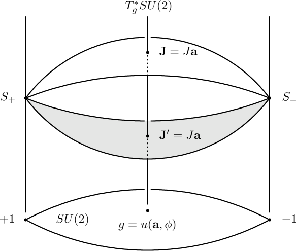
Figure 5: A schematic illustration of the 3-dimensional Lagrangian submanifold $\Lambda_{J}\in T^{*}SU(2)$ for $J>0$. The set $\Lambda_{J}$ consists of two 3-dimensional sections over $SU(2)\setminus\{\pm 1\}$, plus two 2-spheres $S_{+}$ and $S_{-}$ over $\pm 1$. Each section intersects the fiber $T^{*}_{g}SU(2)$ over $g=u({\bf a},\phi)\neq\pm 1$ in one point; on the upper (unshaded) sheet, the point is ${\bf J}=J{\bf a}=-{\bf J}^{\prime}$, while on the lower (shaded) sheet, the point is ${\bf J}=-J{\bf a}=-{\bf J}^{\prime}$.

As for the $B$-manifold in $[{\dot{{\displaystyle T^{*}}SU(2)}}]^{6}$, it is the level set $|{\bf J}_{r}|=J_{r}$, $r=1,\ldots,6$ plus the six diangle conditions, ${\bf J}_{r}+{\bf J}^{\prime}_{r}=0$, $r=1,\ldots,6$, nominally $6+3\times 6=24$ conditions. However, these are not all independent. We examine the question of independence in a single copy of ${\dot{{\displaystyle T^{*}}SU(2)}}$, in which we consider the submanifold defined by ${\bf J}+{\bf J}^{\prime}=0$ and $|{\bf J}|=J$ where $J>0$ is given. We call this submanifold $\Lambda_{J}\subset{\dot{{\displaystyle T^{*}}SU(2)}}$. Let $g\neq\pm 1$ (1 means the identity in $SU(2)$) be a group element, and consider the intersection of the fiber $T_{g}^{*}SU(2)$ over $g$ with $\Lambda_{J}$. Points of this fiber are covectors at $g$, whose components with respect to the right- and left-invariant bases are ${\bf J}$ and $-{\bf J}^{\prime}$. On the intersection these components satisfy ${\bf J}=-{\bf J}^{\prime}$ as well as (95). Since we are assuming ${\bf J}\neq 0$, (95) can only be satisfied if ${\bf J}=-{\bf J}^{\prime}$ is parallel or antiparallel to the axis of the group element $g$. That is, if we write $g$ in axis-angle form, $g=u({\bf a},\phi)$, where ${\bf a}$ is a unit vector, then we must have

$${\bf J}=\pm J{\bf a},\qquad{\bf J}^{\prime}=\mp J{\bf a}.$$ (113)

We exclude $g=\pm 1$ because only for $g\neq\pm 1$ is the axis a unique unit vector in ${\mathbb{R}}^{3}$. Therefore over $SU(2)\setminus\{\pm 1\}$ the manifold $\Lambda_{J}$ consists of two sections of the bundle $T^{*}SU(2)$, so it is 3-dimensional. It is also Lagrangian, being the level set of functions that commute on the level set. As for the points $g=\pm 1$, here $R(g)=I$ (the identity $3\times 3$ rotation) and the intersection of $T_{g}^{*}SU(2)$ with $\Lambda_{J}$ is the 2-sphere $|{\bf J}|=|{\bf J}^{\prime}|=J\neq 0$. This means that the Lagrangian manifold $\Lambda_{J}$ is vertical in two dimensions over $g=\pm 1$ (these points are second order caustics). The two branches of $\Lambda_{J}$ over $SU(2)\setminus\{\pm 1\}$ merge together at $g=\pm 1$, and $\Lambda_{J}$ is connected. The manifold $\Lambda_{J}$ for $J>0$ is illustrated in Fig. 5. Finally, although the set $J=0$ (that is, ${\bf J}=-{\bf J}^{\prime}=0$) is not a part of ${\dot{{\displaystyle T^{*}}SU(2)}}$ it does belong to $T^{*}SU(2)$; it is just the zero section of the bundle, which is diffeomorphic to $SU(2)$ itself, and is therefore 3-dimensional. The manifolds $\Lambda_{J}$ for $J\geq 0$ form a 1-parameter family of 3-dimensional Lagrangian manifolds in $T^{*}SU(2)$.

Finally, the $B$-manifold is the six-fold product $\Lambda_{J_{1}}\times\ldots\times\Lambda_{J_{6}}$; it is an 18-dimensional Lagrangian submanifold of the quotient space $[{\dot{{\displaystyle T^{*}}SU(2)}}]^{6}$.

As for the enlarged manifolds ${\tilde{A}}$ and ${\tilde{B}}$, if we exclude zero edge lengths then these project onto $24$-dimensional submanifolds of $[{\dot{{\displaystyle T^{*}}SU(2)}}]^{6}$. Manifold ${\tilde{A}}$ is specified simply by the four triangle conditions, that is $4\times 3=12$ scalar conditions. As for manifold ${\tilde{B}}$, on a single copy of ${\dot{{\displaystyle T^{*}}SU(2)}}$ let us define

$$\Lambda=\bigcup_{J>0}\Lambda_{J},$$ (114)

which we can extend to $J\geq 0$ on $T^{*}SU(2)$ when relevant. Then $\Lambda$ is a 4-dimensional submanifold of ${\dot{{\displaystyle T^{*}}SU(2)}}$ or $T^{*}SU(2)$, and the manifold ${\tilde{B}}$ is the 24-dimensional subset of $[{\dot{{\displaystyle T^{*}}SU(2)}}]^{6}$ given by $\Lambda^{6}$. It is also the level set of the diangle conditions ${\bf J}_{r}+{\bf J}^{\prime}_{r}=0$, $r=1,\ldots,6$; these are $3\times 6=18$ conditions, the same ones that define ${\tilde{B}}$ as a subset of $\Phi_{12j}$, but only 12 are independent on $[T^{*}SU(2)]^{6}$, as indicated by the fact that ${\tilde{B}}$ is 24-dimensional.

Now we return to Fig. 3 and consider the projection of the manifolds illustrated there onto the quotient space $[{\dot{{\displaystyle T^{*}}SU(2)}}]^{6}$. The projections of the $A$- and $B$-manifolds have just been described; each loses six dimensions upon projection, becoming 18-dimensional, because each is a union of 6-dimensional orbits of the symmetry group $U(1)^{6}$. The same applies to their intersections $T_{1}$ and $T_{2}$, which drop from 15 dimensions to 9. The (projected) 9-dimensional versions of $T_{1}$ and $T_{2}$ on $[{\dot{{\displaystyle T^{*}}SU(2)}}]^{6}$ are the orbits of a 9-dimensional common group, which is worth describing.

The momentum map for the common group consists of the six functions $I_{r}=|{\bf J}_{r}|=|{\bf J}^{\prime}_{r}|$ on $[{\dot{{\displaystyle T^{*}}SU(2)}}]^{6}$, as well as the three functions in ${\bf J}_{\rm tot}$, defined by (21). The group itself is $U(1)^{6}\times SU(2)$. As for the $I_{r}$, the flow of each one acts on only one copy of ${\dot{{\displaystyle T^{*}}SU(2)}}$, and that action was presented in (111) and below. Thus the set of the six $I_{r}$ generates an action of $U(1)^{6}$ with orbits that are 6-tori, upon which the vectors ${\bf J}_{r}$ and ${\bf J}^{\prime}_{r}$ are constant. Since the diangle and triangle conditions depend only on these vectors, if they are satisfied at one point on the 6-torus, they are satisfied at all points on it; thus, the projected $T_{1}$ and $T_{2}$ manifolds in ${\dot{{\displaystyle T^{*}}SU(2)}}$ are unions of such orbits. As for ${\bf J}_{\rm tot}$, this is a sum over $r$ of vectors of the form ${\bf J}+{\bf J}^{\prime}$ for each $r$; the flow generated by each one of these is given by (112). The effect of the $SU(2)$ group action is thus to conjugate each $g_{r}$ by the same element of $SU(2)$, while rotating all of the vectors ${\bf J}_{r}$ and ${\bf J}^{\prime}_{r}$ by the corresponding rotation in $SO(3)$. The latter leaves the diangle and triangle conditions invariant, thus maintaining the conditions for a tetrahedron. Thus, the projected manifolds $T_{1}$ and $T_{2}$ are invariant under this action. Assembling these facts, one can show that the manifolds $T_{1}$ and $T_{2}$ in ${\dot{{\displaystyle T^{*}}SU(2)}}$ consist of precisely one 9-dimensional orbit of the group $U(1)^{6}\times SU(2)$ (for the assumed values of the $J_{r}$).

Finally, the contour $P\to Q\to P^{\prime}\to P$ illustrated in Fig. 3 projects onto a similar contour in $[{\dot{{\displaystyle T^{*}}SU(2)}}]^{6}$. Also, since the symplectic 1-form on $\Phi_{12j}=\Phi_{2j}^{6}$ is the pull-back of that on $[{\dot{{\displaystyle T^{*}}SU(2)}}]^{6}$, the integrals of the symplectic 1-forms along the respective contours are the same. (In general in symplectic reduction, it is only the symplectic 2-forms that are guaranteed to be related by the pull-back, but in this example it works for the 1-forms.) This means that the integral representation of the Ponzano-Regge phase presented in Sec. 3.4) projects onto $[{\dot{{\displaystyle T^{*}}SU(2)}}]^{6}$.

Similarly, the manifolds illustrated in Fig. 4 also project onto $[{\dot{{\displaystyle T^{*}}SU(2)}}]^{6}$, losing six dimensions in the process. The proof of the Schläfli identity given in Sec. 4 and based on these manifolds also carries over to the quotient space with just a change of context. One of the manifolds used in this proof is ${\tilde{T}}$, which is the union of all manifolds $T_{1}$ and $T_{2}$ for all values of the $J_{r}$ (we may exclude $J_{r}=0$). This is the manifold of tetrahedra, and being a 6-parameter family of 9-dimensional manifolds, it is 15-dimensional.

5.9 Semiclassical Interpretation of $\Lambda_{J}$

We make some final remarks of a semiclassical nature concerning the Lagrangian manifolds $\Lambda_{J}\subset T^{*}SU(2)$. Whenever a Lagrangian manifold occurs in a classical context it is useful to ask what its semiclassical significance is. In the case of the $\Lambda_{J}$ it is easiest to answer this question with respect to the version of $T^{*}SU(2)$ obtained from $\Phi_{2j}^{*}$ rather than from $\Phi_{2j}$. In the following we will proceed somewhat intuitively, stating several plausible facts without proof and switching back and forth between the classical geometry and the corresponding objects and operations in the linear algebra of the corresponding quantum systems.

For a given $J$, $\Lambda_{J}\subset T^{*}SU(2)$ is the 3-dimensional level $I=|{\bf J}|=J$, ${\bf J}={\bf J}^{\prime}$. Let us denote its preimage under the projection map $:{\dot{L}}\to{\dot{{\displaystyle T^{*}}SU(2)}}$ by $M_{J}$, which is the level set $I=J$, ${\bf J}={\bf J}^{\prime}$ inside $\Phi_{2j}^{*}$. Then $M_{J}\subset{\dot{L}}\subset\Phi_{2j}^{*}$, and $M_{J}$ is a 4-dimensional Lagrangian manifold in $\Phi_{2j}^{*}$. It will be easiest to explain the semiclassical significance of $M_{J}$ first, and then to turn to $\Lambda_{J}$.

We denote the Hilbert space of two harmonic oscillators by ${\cal H}$ as above. As explained by Schwinger (1952) and Bargmann (1962), ${\cal H}$ carries a unitary representation of $SU(2)$ which we denote by $g\mapsto U(g)$, and under this action ${\cal H}$ decomposes into one carrier space of irrep $j$ for each $j$,

$${\cal H}=\bigoplus_{j}{\cal H}_{j}.$$ (115)

A convenient basis on ${\cal H}$ is $\{|jm\rangle,\forall j,m\}$, where “$\forall j,m$” means all $j$ and $m$ allowed by the usual restrictions on angular momentum quantum numbers. A basis in ${\cal H}_{j}$ is the restricted set $\{|jm\rangle,\forall m\}$.

The Hilbert space corresponding to $\Phi_{2j}^{*}$ is ${\cal H}\otimes{\cal H}^{*}$, that is, it consists of linear combinations of vectors of the form $|\phi\rangle\langle\psi|$, in Dirac notation. These vectors are otherwise linear operators $:{\cal H}\to{\cal H}$. A convenient basis on ${\cal H}\otimes{\cal H}^{*}$ is the set $\{|jm\rangle\langle j^{\prime}m^{\prime}|,\forall j,j^{\prime},m,m^{\prime}\}$. Now the subset of $\Phi_{2j}^{*}$ indicated by $I=I^{\prime}$, that is, the set $L\subset\Phi_{2j}^{*}$, corresponds to the subspace of ${\cal H}\otimes{\cal H}^{*}$ on which $j=j^{\prime}$. Let us call this space ${\cal L}\subset{\cal H}\otimes{\cal H}^{*}$. Space ${\cal L}$ is spanned by $\{|jm\rangle\langle jm^{\prime}|,\forall j,m,m^{\prime}\}$, and it contains the operators $:{\cal H}\to{\cal H}$ that leave each irreducible subspace ${\cal H}_{j}$ invariant. That is, the operators in ${\cal L}$ are are block diagonal in the $|jm\rangle$ basis. In summary, ${\cal L}$ is the space of operators corresponding semiclassically to the manifold $L$.

Restricting the level set further by requiring that $I=I^{\prime}=J$ for a given $J$, we obtain a classical submanifold of $\Phi_{2j}^{*}$ that corresponds to operators that are linear combinations of the set $\{|jm\rangle\langle jm^{\prime}|,\forall m,m^{\prime}\}$, that is, operators in ${\cal L}$ with a fixed value of $j$. These operators map ${\cal H}_{j}$ into itself for the given $j$, while annihilating all vectors in ${\cal H}_{j^{\prime}}$ for $j^{\prime}\neq j$. Let us call this space ${\cal L}_{j}\subset{\cal L}$; it has dimensionality $(2j+1)^{2}$.

Restricting the level set $I=I^{\prime}=J$ further by adding ${\bf J}={\bf J}^{\prime}$, we obtain the classical manifold $M_{J}$. On the Hilbert space ${\cal H}\otimes{\cal H}^{*}$ the operators ${\bf J}-{\bf J}^{\prime}$ generate an action of $SU(2)$ given by $X\mapsto U(g)XU(g)^{\dagger}$, where $X:{\cal H}\to{\cal H}$ is any operator. Also, the condition ${\bf J}-{\bf J}^{\prime}=0$ specifies a subspace of operators for which $U(g)XU(g)^{\dagger}=X$, that is, operators that are invariant under rotations. But the only operator in ${\cal L}_{j}$ that is invariant under rotations is the projection operator onto subspace ${\cal H}_{j}$,

$$\Pi_{j}=\sum_{m}|jm\rangle\langle jm|,$$ (116)

according to Schur’s lemma. This is the operator or vector in ${\cal L}_{j}\subset{\cal L}\subset{\cal H}\otimes{\cal H}^{*}$ that corresponds to the classical Lagrangian manifold $M_{J}$.

Now we turn to the projection of $L$ onto $T^{*}SU(2)$ and of $M_{J}\subset L$ onto $\Lambda_{J}\subset T^{*}SU(2)$, and explain the corresponding linear algebra. The symplectic manifold $T^{*}SU(2)$ is the cotangent bundle of $SU(2)$, so it should be the phase space corresponding to $L^{2}(SU(2))$, the Hilbert space of wave functions on $SU(2)$. An obvious basis on this Hilbert space is the set of components of the rotation matrices, $\{D^{j}_{mm^{\prime}}(g),\forall j,m,m^{\prime}\}$, which are orthonormal with respect to the Haar measure on the group. Actually, it is better to use the complex conjugates of these functions on $SU(2)$, $\overline{D^{j}_{mm^{\prime}}(g)}$, which, when regarded as wave functions of a rigid body, have the correct transformation properties under rotations (Littlejohn and Reinsch 1997). In view of the quantum numbers, these wave functions are obviously the images of the vectors $|jm\rangle\langle jm^{\prime}|$ under the quantum analog of the classical projection map, and it would appear that we have a map $:{\cal L}\to L^{2}(SU(2))$.

Explicitly, this map is

$$X\mapsto\psi_{X}(g)=\tr[U(g)^{\dagger}X],$$ (117)

where $X\in{\cal L}$. In particular, the basis vector $|jm\rangle\langle jm^{\prime}|$ is mapped into

$$\tr[U(g)^{\dagger}|jm\rangle\langle jm^{\prime}|]=\langle jm^{\prime}|U(g)^{\dagger}|jm\rangle=\overline{D^{j}_{mm^{\prime}}(g)},$$ (118)

as expected. As for the projection operator $\Pi_{j}$, its wave function on $SU(2)$ is the character,

$$\Pi_{j}\mapsto\tr[U(g)^{\dagger}\Pi_{j}]=\sum_{m}\overline{D^{j}_{mm}(g)}=\chi^{j}(g),$$ (119)

where $\chi^{j}(g)$ actually depends only on the conjugacy class, and where we have used the fact that for $SU(2)$ the characters are real. Thus we see that the wave function on $SU(2)$ corresponding to the Lagrangian manifold $\Lambda_{J}$ is the character $\chi^{j}(g)$.

The trace in (117) is the scalar product in ${\cal H}\otimes{\cal H}^{*}$, so semiclassically its stationary phase points should be the intersections of the Lagrangian manifolds in $\Phi_{2j}^{*}$ corresponding to operators $X$ and $U(g)$. As for $U(g)$, its Lagrangian manifold is $z=gz^{\prime}$, precisely the coordinate transformation we used in Sec. 5.3 on passing from ${\dot{L}}$ to ${\dot{{\displaystyle T^{*}}SU(2)}}$. One way to see this is to note that the graph of a symplectic map $:\Phi\to\Phi$ in $\Phi\times\Phi^{*}=\Phi_{2j}^{*}$ is a Lagrangian manifold in the latter space. In this case, $z=gz^{\prime}$, which is the obvious symplectic map corresponding to $U(g)$, specifies a Lagrangian manifold in $\Phi_{2j}^{*}$ that is the obvious candidate for the manifold supporting the operator $U(g)$. The fact that it is Lagrangian can be verified directly by computing the Poisson brackets among the components of $z-gz^{\prime}$ and $z^{\dagger}-z^{\prime\dagger}g^{\dagger}$ in the symplectic structure (47). These Poisson brackets all vanish. The Lagrangian manifold $z-gz^{\prime}=0$ in $\Phi_{2j}^{*}$ is actually a plane, which moreover is a subset of $L$.

Another point of view is the following. The operator $U(g)$ belongs to the space ${\cal H}\otimes{\cal H}^{*}$. Let us call operators in this space “ordinary operators,” while linear operators mapping this space into itself we will call “superoperators” (terminology without relation to supersymmetry). Then an ordinary operator can be associated with a superoperator by either left or right multiplication. For example, the ordinary operator $a_{\mu}$, the usual annihilation operator, becomes a superoperator by either left or right multiplication, $X\mapsto a_{\mu}X$ or $X\mapsto Xa_{\mu}$, where $X$ is an ordinary operator. Then on the phase space $\Phi_{2j}^{*}$ the superoperator, left multiplying by $a_{\mu}$, has Weyl symbol $z_{\mu}$, while the superoperator, right multiplying by $a_{\mu}$, has Weyl symbol $z^{\prime}_{\mu}$, in the $(z,z^{\prime})$ coordinates we have been using on $\Phi_{2j}^{*}$. These operators satisfy the relation,

$$a_{\mu}U(g)=U(g)\sum_{\nu}g_{\mu\nu}\,a_{\nu},$$ (120)

which can be expressed by saying that $U(g)$ is an eigenoperator of the commuting superoperators whose symbols are the components of $z-gz^{\prime}$ with eigenvalues 0. Thus $U(g)$ is supported semiclassically by the Lagrangian manifold $z=gz^{\prime}$.

The Lagrangian manifold $z=gz^{\prime}$ in $\Phi_{2j}^{*}$ is a subset of $L$ and moreover consists of orbits of $I-I^{\prime}$. Thus it survives the projection onto the quotient space, where in fact it becomes simply $g={\rm const}$ on $T^{*}SU(2)$. That is, it is the fiber over the point $g$ in the cotangent bundle. This fiber is naturally Lagrangian. So the intersections of Lagrangian manifolds implied by (117) projects onto an intersection of Lagrangian manifolds in $T^{*}SU(2)$, one being $\Lambda_{J}$ and the other the fiber over $g$ in $T^{*}SU(2)$. This is the expected geometry for a wave function on $SU(2)$.

Finally we note that the characters in $SU(2)$ are given explicitly by

$$\chi^{j}(\phi)=\frac{\sin(j+1/2)\phi}{\sin(1/2)\phi},$$ (121)

where we write $g$ in axis-angle form, $g=u({\bf a},\phi)$. By tracking the Lagrangian manifolds and the densities on them through the projection process we have just described it can be shown that the denominator $\sin(1/2)\phi$ can be interpreted as an amplitude determinant in the semiclassical expression for the wave function. The amplitude diverges at $\phi=0$ and $\phi=2\pi$, that is, at the group elements $g=\pm 1$, where as we have noted the Lagrangian manifold has caustics when projected onto the base space $SU(2)$. The numerator $\sin(j+1/2)\phi$ is the sum of two branches of a WKB wave function, corresponding to the two branches of $\Lambda_{J}$ seen in Fig. 5 or in Fig. 7 below.

In the case of the character formula the semiclassical treatment is exact. This can be seen as an example of the Duistermaat-Heckman theorem, which also connects this discussion with mathematical work on the asymptotics of group structures. See Duistermaat and Heckman (1982), Thompson and Blau (1997), Stone (1989) and Ben Geloun and Gurau (2011).

6 The Second Reduction

We now carry out a second reduction, this one taking us from $[{\dot{{\displaystyle T^{*}}SU(2)}}]^{6}$ or $[T^{*}SU(2)]^{6}$ to a new quotient space we denote by ${\dot{\Sigma}}$ or $\Sigma$. It will turn out that $\Sigma$ is essentially the symplectic manifold found in an ad hoc manner in Sec. 2 and illustrated in Fig. 1. The symmetry group for this reduction is $SU(2)^{6}$, and its momentum map and the level set to be used are given by ${\bf J}_{r}+{\bf J}^{\prime}_{r}=0$, $r=1,\ldots,6$.

Before we develop this further, however, there is one obvious problem, if we intend to project the contour for the Ponzano-Regge phase, illustrated in Fig. 3, onto ${\dot{\Sigma}}$. That is, although the $B$-manifold is a subset of the level set ${\bf J}_{r}+{\bf J}^{\prime}_{r}=0$, $r=1,\ldots,6$, as required if it is to survive the projection onto ${\dot{\Sigma}}$, the same does not apply to the $A$-manifold. Therefore we do not seem to have a contour for the Ponzano-Regge phase on ${\dot{\Sigma}}$. We address this problem before studying the second reduction further.

6.1 A New Contour for the Ponzano-Regge Phase

Consider the contour $P\to Q\to P^{\prime}\to P$ illustrated in Fig. 3. It was explained in Sec. 3 that the integral of the symplectic 1-form $\theta$ around this contour is $2S$, where $S$ is the Ponzano-Regge phase given by (7). In this section we interpret this contour as belonging to either $\Phi_{12j}$ or ${\dot{{\displaystyle T^{*}}SU(2)}}\subset T^{*}SU(2)$ and $\theta$ as given by either (15) or (94). However, it was also pointed out in Sec. 3 that the integrals of $\theta$ along the legs $P\to Q$ and $Q\to P^{\prime}$ vanish, so in fact the closed contour $P\to Q\to P^{\prime}\to P$ can be restricted to just the open contour $P^{\prime}\to P$ without changing the result. The latter contour is an open contour contained in the intersection set $T_{1}$.

Figure 6: A reduced contour $C$ for the Ponzano-Regge phase. The contour lies entirely inside the set ${\tilde{T}}$ of tetrahedra.

Next, in Sec. 4 a family of such contours, parameterized by $\lambda$, was considered, as illustrated in Fig. 4. These sweep out a 2-dimensional surface illustrated in the figure. Applying Stokes’ theorem to the integral of $\omega=d\theta$ over this surface (the “walls”), we find that this integral is $2[S(\lambda_{1})-S(\lambda_{0})]$. On the other hand, it was pointed out in Sec. 4 that the integrals of $\omega$ over the first and second legs of the surface vanish, as indicated by (36). Now applying Stokes’ theorem to the integral over the third leg only, we obtain

$$2[S(\lambda_{1})-S(\lambda_{0})]=\int_{C}\theta,$$ (122)

where $C$ is the closed contour $P(\lambda_{0})\to P^{\prime}(\lambda_{0})\to P^{\prime}(\lambda_{1})\to P(\lambda_{1})\to P(\lambda_{0})$ which may be seen in Fig. 4 and which is illustrated separately in Fig. 6. In fact, the integral along the top and bottom edges of $C$ give the result shown in (122), so the integrals of $\theta$ along the vertical segments in Fig. 6 must cancel each other.

For our purposes the main point is that this new contour $C$ lies entirely in the space ${\tilde{T}}$ of tetrahedra. This is a subset of ${\tilde{B}}$, which survives the projection onto ${\dot{\Sigma}}$, so the contour $C$ illustrated in Fig. 6 does also, and gives us an integral representation of the Ponzano-Regge phase (actually the difference seen in (122)) on the quotient space ${\dot{\Sigma}}$.

Before leaving this contour we will specialize the initial conditions for future convenience. The 2-dimensional surface illustrated in Fig. 4 is swept out by curves $P(\lambda)\to Q(\lambda)\to P^{\prime}(\lambda)\to P(\lambda)$. All we require of the initial point $P(\lambda)$ is that it lie in the space ${\tilde{T}}$ of tetrahedra, that is, that the triangle and diangle conditions be satisfied. Supposing this to be true, there still remains the question of the initial phases of the spinors $(z_{r},z^{\prime}_{r})$. Let us now assume that at $P(\lambda)$, $z^{\prime}_{r}=\zeta_{r}$, where $\zeta_{r}$ is a spinor such that $(1/2)\zeta_{r}^{\dagger}\boldsymbol{\sigma}\zeta_{r}={\bf J}^{\prime}_{r}$. Let us also assume that at $P(\lambda)$, $z_{r}=\Theta\zeta_{r}$. This implies $(1/2)z_{r}\boldsymbol{\sigma}z_{r}={\bf J}_{r}=-{\bf J}^{\prime}_{r}$, as required of the initial conditions.

Then the procedure of Sec. 3 shows that at point $P^{\prime}(\lambda)$, we have $z^{\prime}_{r}=\zeta_{r}$ (the same as at $P(\lambda)$), and $z_{r}=e^{i\psi_{r}}\Theta\zeta_{r}$, where $\psi_{r}=\psi_{r}(\lambda)$ is the dihedral angle of edge $r$ of the initial tetrahedron. Thus, one can say that the contour $C$ illustrated in Fig. 6 has the dihedral angles built into it.

These choices are convenient, because they imply that at $P(\lambda)$ (and therefore all along the segment $P(\lambda_{1})\to P(\lambda_{0})$ in Fig. 6) we have $g_{r}=1$, $r=1,\ldots,6$. As for point $P^{\prime}(\lambda)$, we have

$$g_{r}=u({\bf j}_{r},-2\psi_{r})=u(-{\bf j}_{r},2\psi_{r}),$$ (123)

because this $SU(2)$ element, when applied to $\Theta\zeta_{r}$, brings out the phase $e^{i\psi_{r}}$. Here ${\bf j}_{r}={\bf J}_{r}/J_{r}$.

6.2 Back to the Second Reduction

We now carry out the second reduction, in which the group is $SU(2)^{6}$, generated by ${\bf J}_{r}+{\bf J}^{\prime}_{r}$, $r=1,\ldots,6$. We work on the level set ${\bf J}_{r}+{\bf J}^{\prime}_{r}=0$, which is otherwise ${\tilde{B}}$. For simplicity we work with the space $[T^{*}SU(2)]^{6}$ rather than $[{\dot{{\displaystyle T^{*}}SU(2)}}]^{6}$. As before the group action is a product of an action on each factor, in this case $SU(2)$ acting on $T^{*}SU(2)$; the latter action is given explicitly by (112). We drop the $r$ index when considering a single factor.

The zero level set in the 6-dimensional space $T^{*}SU(2)$ is $\Lambda$, defined by (114); it is 4-dimensional. When considering the action of $SU(2)$ on $\Lambda$ it is convenient to decompose $\Lambda$ into the family of 3-dimensional submanifolds $\Lambda_{J}$, as indicated by (114), since each $\Lambda_{J}$ is invariant under the same action. See Fig. 5. To show this explicitly, consider a point $g=u({\bf a},\phi)\neq\pm 1$ as in the figure, so that the action (112) implies

$$g=u({\bf a},\phi)\mapsto u({\bf n},\alpha)u({\bf a},\phi)u({\bf n},\alpha)^{-1}=u({\bf b},\phi),$$ (124)

where ${\bf b}=R({\bf n},\alpha){\bf a}$. That is, the axis of the rotation transforms the same as ${\bf J}$ and ${\bf J}^{\prime}$, so the conditions ${\bf J}=\pm J{\bf a}$, ${\bf J}^{\prime}=\mp J{\bf a}$ are maintained by the action (112). As for the points $g=\pm 1$, the 2-spheres over these points (sets $S_{+}$ and $S_{-}$ in the diagram) are invariant under the action (112). It is also easy to see that $\Lambda_{J}$ for $J=0$ is invariant under the action. Since all sets $\Lambda_{J}$ are invariant under the action, so is $\Lambda$, and the isotropy subgroup is the entire group $SU(2)$.

As for the orbits of the action, consider first $J>0$ and $g\neq\pm 1$. Then the action (112) causes the point $g$ to sweep out a conjugacy class in $SU(2)$, which is a 2-sphere; and the point on $\Lambda_{J}$ over $g$ on either (upper or lower) section sweeps out the portion of the section over the conjugacy class. But since proper rotations cannot connect ${\bf J}=J{\bf a}$ with ${\bf J}=-J{\bf a}$, the orbits of the action (112) lie entirely on the upper or lower sections, and the two branches are not connected by the action. Thus the orbits are copies of the conjugacy class over which they lie, and are 2-spheres. Similarly, over the points $g=\pm 1$ the orbits are 2-spheres, so all orbits for $J>0$ are 2-spheres. As for the set $\Lambda_{J}$ for $J=0$, the orbits are the conjugacy classes, which are 2-spheres except at $g=\pm 1$ where they are single points.

Figure 7: Illustration of the quotient space $\Lambda_{J}/SU(2)$ for the case $J>0$. The space is a circle, which can be regarded as a two-branched object over the space $0<\phi<2\pi$ of conjugacy classes, with the two branches joining at $\phi=0$ and $\phi=2\pi$. The upper branch represents the part of the cotangent bundle $T^{*}SU(2)$ over the conjugacy class for which ${\bf J}=+J{\bf a}$ and ${\bf J}^{\prime}=-J{\bf a}$, while on the lower branch ${\bf J}=-J{\bf a}$ and ${\bf J}^{\prime}=+J{\bf a}$.

To parameterize the conjugacy classes of $SU(2)$ we write $g=u({\bf a},\phi)$ so that $\phi$ in the range $0\leq\phi\leq 2\pi$ is a coordinate of the conjugacy classes, with $\phi=0$ meaning $g=1$ and $\phi=2\pi$ meaning $g=-1$. Then to construct the quotient space we take first the case $J>0$, for which $\Lambda_{J}$ is 3-dimensional and all orbits are 2-spheres, so that the quotient space is 1-dimensional. It consists of two branches over $0<\phi<2\pi$, corresponding to ${\bf J}=\pm J{\bf a}$, which join together in a single branch over $\phi=0$ and $\phi=2\pi$, as illustrated in Fig. 7. The quotient space $\Lambda_{J}/SU(2)$ for $J>0$ is a circle. We introduce a coordinate $\tau$ on this circle by defining $\tau=\phi$ on the upper branch where ${\bf J}=J{\bf a}$, and $\tau=-\phi$ on the lower branch where ${\bf J}=-J{\bf a}$. Then we can take $\tau$ in the range $-2\pi<\tau\leq 2\pi$. This takes care of the case $J>0$.

Forming the union of these circles for all $J>0$, we obtain a cylinder with coordinates $(J,\tau)$, $0<J<\infty$. This is the quotient manifold under the second symplectic reduction applied to ${\dot{{\displaystyle T^{*}}SU(2)}}$. At $J=0$ the set $\Lambda_{J}$ is just $SU(2)$ itself, and the quotient space is the one-dimensional interval $0\leq\phi\leq 2\pi$, the set of conjugacy classes. Therefore we can pinch off the cylinder at $J=0$ into this interval to form the entire quotient space. Alternatively, since the set $J=0$ was a single point of the level set in the first reduction and the set $\Lambda_{J}$ for $J=0$ is not a part of the image of the first reduction, it is reasonable to take care of the case $J=0$ in an ad hoc manner by pinching off the cylinder at $J=0$ into a point. The resulting set is topologically ${\mathbb{R}}^{2}$, with polar coordinates $(J,\tau)$ with $-2\pi<\tau\leq 2\pi$. Recall also that the case $J=0$ means a tetrahedron for which the dihedral angles are not defined, so it plays no role in the Schläfli identity.

Extending this construction to all values of $r=1,\ldots,6$, we can define the quotient space ${\dot{\Sigma}}$ as the sixth power of the cylinder with coordinates $(J,\tau)$ just described; and similarly, we define $\Sigma$ as the sixth power of the plane ${\mathbb{R}}^{2}$ with polar coordinates $(J,\tau)$.

6.3 The Symplectic Form on $\Sigma$ or ${\dot{\Sigma}}$

To compute the symplectic form on the $(J,\tau)$ cylinder we first restrict the form (93) to the level set, upon which ${\bf J}=\pm J{\bf a}$. This gives

$$\theta=i{\bf J}\cdot\tr(\boldsymbol{\sigma}\,dg\,g^{\dagger})=\pm iJ\tr[dg\,g^{\dagger}({\bf a}\cdot\boldsymbol{\sigma})].$$ (125)

But $g=\cos\phi/2-i({\bf a}\cdot\boldsymbol{\sigma})\sin\phi/2$, so

$$g^{\dagger}({\bf a}\cdot\boldsymbol{\sigma})=({\bf a}\cdot\boldsymbol{\sigma})\cos\phi/2+i\sin\phi/2.$$ (126)

Also,

$$dg=\frac{1}{2}[-\sin\phi/2-i({\bf a}\cdot\boldsymbol{\sigma})\cos\phi/2]d\phi-i(d{\bf a}\cdot\sigma)\sin\phi/2.$$ (127)

Now upon substituting (127) into (125) the term involving $d{\bf a}$ vanishes, since ${\bf a}\cdot d{\bf a}=0$ (${\bf a}$ is a unit vector) and since $\tr\boldsymbol{\sigma}=0$. As for the term in $d\phi$, it gives

$$\theta=\pm J\,d\phi,$$ (128)

after a bit of algebra, where the $\pm$ sign refers to the upper or lower branches. But this can be expressed in terms of the coordinate $\tau$ on the circles, giving

$$\theta=J\,d\tau.$$ (129)

This is the symplectic form on the cylinder, or the plane ${\mathbb{R}}^{2}$, if we extend it to $J=0$ in the manner suggested above. It looks like the symplectic form for the harmonic oscillator in action-angle variables, except that the angle $\tau$ has a range of $4\pi$.

Taking the sixth power of this, we obtain the symplectic 1-form on $\Sigma$ or ${\dot{\Sigma}}$, which is

$$\theta=\sum_{r}J_{r}\,d\tau_{r}.$$ (130)

Figure 8: When the contour illustrated in Fig. 6 is projected onto the quotient space ${\dot{\Sigma}}$, and then projected again onto one of the $J$-$\tau$ spaces for some $r$, it becomes the contour illustrated here. On the upper segment $J=J(\lambda_{1})$ and on the lower $J=J(\lambda_{0})$, while on the vertical segment at the left, $\tau=-2\psi(\lambda)$ and $J=J(\lambda)$.

6.4 The Contour and Lagrangian Manifold on ${\dot{\Sigma}}$

Now let us project the contour illustrated in Fig. 6 onto the reduced space. The contour contains a path $P(\lambda_{1})\to P(\lambda_{0})$, along which ${\bf J}_{r}$ and ${\bf J}^{\prime}_{r}$ are functions of $\lambda$, defining a family of tetrahedra for which (by our assumptions) $V>0$; therefore, along this path, $J_{r}$ and $\psi_{r}$ are functions of $\lambda$, with $J_{r}>0$. Also, according to the conventions introduced in Sec. 6.1, we have $g_{r}=1$ along this path, and hence $\tau_{r}=0$. Next, along the path $P(\lambda_{0})\to P^{\prime}(\lambda_{0})$, $J_{r}$ is constant while the group element $g_{r}$ has axis ${\bf a}=-{\bf j}_{r}$ and an angle (or conjugacy class) $\phi$ that goes from 0 to $2\psi_{r}$, as indicated by (123). This means that ${\bf J}=-J{\bf a}$, so we are on the lower branch of Fig. 7, and $\tau_{r}$ goes from 0 to $-2\psi_{r}(\lambda_{0})$. The path $P^{\prime}(\lambda_{1})\to P(\lambda_{1})$ is similar; $J_{r}$ is constant along this path, and $\tau_{r}$ goes from $-2\psi_{r}(\lambda_{1})$ to 0. Finally, along the path $P(\lambda_{0})\to P(\lambda_{1})$, $J_{r}$ and $\tau_{r}$ are functions of $\lambda$, with $\tau_{r}=-2\psi_{r}(\lambda)$. This projected contour lies in the space ${\dot{\Sigma}}$ or $\Sigma$; when it is projected onto one of the $(J,\tau)$ spaces for a fixed $r$, we obtain Fig. 8.

Finally, the manifold on ${\dot{\Sigma}}$ given by $\tau_{r}=-2\psi_{r}$, where the $\psi_{r}$ are functions of the six $J_{r}$’s, is a Lagrangian manifold, according to the logic of Sec. 2. In fact, ${\dot{\Sigma}}$ is essentially the symplectic manifold constructed in Sec. 2, apart from signs and factors of 2. A surprising aspect of this result is that the dihedral angles of the tetrahedron emerge in the end as labels of conjugacy classes in $SU(2)$.

7 Conclusions

To conclude we will mention some aspects of this calculation that have not been mentioned so far. First, it would be possible to carry out the two symplectic reductions of this paper in a single step, that is, by taking the momentum map and level set to be ${\bf J}_{r}+{\bf J}^{\prime}_{r}=0$, specifying the first and only reduction. This condition implies $I_{r}=I^{\prime}_{r}$, so it includes the first reduction as carried out in this paper. We have proceeded in two steps because it is easier to see how the reductions work this way, and because the intermediate stage, which involves $T^{*}SU(2)$, is interesting in its own right, with potential applications in quantum gravity.

Another possibility is to reduce the original problem by $I_{r}=I^{\prime}_{r}=J_{r}$, which means a set of twelve copies of the Hopf fibration, resulting in a reduced phase space which is $(S^{2}\times S^{2})^{6}$, in which the twelve angular momentum vectors ${\bf J}_{r}$ and ${\bf J}^{\prime}_{r}$, with fixed magnitudes, are coordinates. In this case the Ponzano-Regge phase can be expressed as a contour along 12-dimensional Lagrangian manifolds in this 24-dimensional space, and the dihedral angles appear as solid angles of wedges on spheres. This phase space can then be reduced again by ${\bf J}_{\rm tot}$, which produces a phase space that is closely related to the shape spaces, ${\cal S}$ and ${\dot{\cal S}}$.

Thus far we have restricted attention to the Schläfli identity in Euclidean ${\mathbb{R}}^{3}$. Schläfli’s original proof treated the case of the constantly curved three-sphere $S^{3}$, Schläfli (1858). In fact, similar identities hold in each of the three-dimensional constant curvature spaces, including hyperbolic three-space $\mathbb{H}^{3}$, as well as in arbitrary dimensions; the metrical proofs of Milnor (1994) and Alekseevskij, Vinberg and Solodovnikov (1993) already mentioned treat the general case where the sectional curvature $\kappa$ is variable. If we parameterize this curvature with $\kappa=-1,0,1$ for $\mathbb{H}^{3}$, $\mathbb{R}^{3}$ and $S^{3}$ respectively, then all three identities can be summarized in a single formula

$$2\kappa dV=\sum_{r}J_{r}d\psi_{r}.$$ (131)

We believe that the symplectic method of proof described in this paper can be generalized to an arbitrary constant curvature three space. This is briefly outlined in the following paragraphs and will be described more fully in a future publication.

Once again, we define a tetrahedron in each of the constant curvature spaces $\mathbb{H}^{3}$ and $S^{3}$ through an ordered set of four vertices. We connect the vertices by geodesic arcs and view these arcs as subsets of completely geodesic surfaces that make up the faces of the tetrahedron. The curved space versions of the Schläfli identity apply to these curved tetrahedra.

Just as a Euclidean tetrahedron emerges from the asymptotics of the ordinary Wigner $6j$-symbol, a tetrahedron in spaces of constant (positive or negative) curvature emerges from the asymptotics of the $q$-deformed $6j$-symbol, an invariant in the representation theory of the quantum group or Hopf algebra $\mathfrak{su}(2)_{q}$ (Chari and Pressley 1994). This much is clear already from the work of Mizoguchi and Tada (1992) and of Taylor and Woodward (2005), both of whom used one-dimensional WKB techniques along the lines of Schulten and Gordon (1975ab).

These asymptotics are important in quantum gravity. A number of works have drawn connections between the $q$-deformed symbols and discretizations of general relativity that include a cosmological constant. In connection with loop quantum gravity Han (2011) and Fairbairn and Meusberger (2011) have developed $q$-deformed spin foam models and Dupuis and Girelli (2013), Bonzom et al(2014a), Bonzom et al(2014b) and Dupuis et al(2014) have developed further connections between the geometry of $q$-deformation and the cosmological constant.

A fully symplectic derivation of these asymptotics has yet to appear and this is part of what we would like to achieve in our future work. We will now outline some progress in this direction, speaking of the case of real $q>0$, which corresponds to tetrahedral geometry in the hyperbolic space $\mathbb{H}^{3}$.

The Hopf algebra $\mathfrak{su}(2)_{q}$ is generated by three operators, $J_{z}$ and $J_{\pm}$, satisfying the commutation relations,

$$\eqalign{[J_{z},J_{\pm}]&=\pm\hbar\,J_{\pm},\cr[J_{+},J_{-}]&=\hbar\,\frac{q^{J_{z}/\hbar}-q^{-J_{z}/\hbar}}{q^{1/2}-q^{-1/2}}}$$ (132)

where in comparison to the usual formulas we have inserted factors of $\hbar$, assuming that $J_{z}$, $J_{\pm}$ have dimensions of angular momentum. This algebra can be realized in terms of the raising and lowering operators of a $q$-deformed harmonic oscillator, in a generalization of the Schwinger-Bargmann representation of $SU(2)$, as shown by Biedenharn (1989) and Macfarlane (1989). We follow Biedenharn’s convention for $q$ in (132). The $q$-deformed $6j$-symbol is constructed out of irreducible representations of this algebra, labeled by six values of the quantum number $j$, in a manner similar to that used to construct the ordinary $6j$-symbol out of six irreps of $SU(2)$. In fact, the $q$-deformed symbol approaches the ordinary one as $q\to 1$, just as the Hopf algebra (132) approaches the ordinary Lie algebra $\mathfrak{su}(2)$ in the same limit.

To study the asymptotics of the representations of the algebra (132) we wish to take the limit $\hbar\to 0$. This limit does not exist if $q$ is held fixed, because of the terms $q^{\pm J_{z}/\hbar}$. To obtain a well defined limit we follow Mizoguchi and Tada (1992) and Taylor and Woodward (2005) by scaling $q$ along with $\hbar$. We do this by requiring that the ratio

$$J_{0}=\frac{\hbar}{\log q}$$ (133)

be held fixed in the limit $\hbar\to 0$. With this understanding the limit $\hbar\to 0$ converts the operator algebra (132) into the Poisson algebra

$$\eqalign{\{J_{z},J_{x}\}&=J_{y},\qquad\{J_{z},J_{y}\}=-J_{x},\cr\{J_{x},J_{y}\}&=J_{0}\sinh(J_{z}/J_{0}),}$$ (134)

where $J_{\pm}=J_{x}\pm iJ_{y}$. In these Poisson bracket relations the operators $(J_{x},J_{y},J_{z})$ have been “dequantized,” that is, they are no longer linear operators but rather functions on the phase space $\Phi$ of the 2-dimensional $q$-deformed harmonic oscillator. We do not give the definitions of these functions here but they are the dequantization of the formulas given by Biedenharn (1989) and Macfarlane (1989) for the $J$-operators in terms of the $q$-deformed raising and lowering operators. As for $J_{0}$, it plays the role of the curvature of the hyperbolic space $\mathbb{H}^{3}$. If we like we can set $J_{0}=1$, corresponding to the standard case $\kappa=-1$ in (131), or we can keep $J_{0}$ which is useful for studying the limit $J_{0}\to\infty$ which is the nondeformed case $q=1$.

The definitions of $(J_{x},J_{y},J_{z})$ provide a map from the phase space $\Phi$ to ${\mathbb{R}}^{3}$, in which the $J$’s are coordinates (this is a generalization of the Hopf map discussed below (9)). The Poisson bracket relations (134) mean that this version of ${\mathbb{R}}^{3}$ is a Poisson manifold. In the nondeformed case ($q=1$), the resulting space is $\mathfrak{su}(2)^{*}$, the dual of the Lie algebra of $SU(2)$, otherwise “angular momentum space.” This is a vector space, hence an Abelian group under addition. In the deformed case, the space with $(J_{x},J_{y},J_{z})$ as coodinates is a non-Abelian group, isomorphic to the subgroup of $SL(2,{\mathbb{C}})$ consisting of upper triangular matrices with real diagonal elements. We call this group $B$; the identification of angular momentum space with matrices in $B$ is specified by the matrix

$$b=\left(\begin{array}[]{cc}e^{-J_{z}/2}&-J_{-}\cr 0&e^{J_{z}/2}\end{array}\right)\in B,$$ (135)

where we have set $J_{0}=1$. Since these are elements of $SL(2,{\mathbb{C}})$ they correspond to Lorentz transformations and thus have an action on the unit mass shell in Minkowski ${\mathbb{R}}^{4}$, which otherwise is a realization of the hyperbolic space $\mathbb{H}^{3}$. By this action “angular momentum space” in the deformed case, previously identified with ${\mathbb{R}}^{3}$, is seen to be diffeomorphic to $\mathbb{H}^{3}$, which is a more useful identification. The group $B\subset SL(2,{\mathbb{C}})$ plays a role in the Iwasawa decomposition of $SL(2,{\mathbb{C}})$ (Helgason 1978), in which an arbitrary element of $SL(2,{\mathbb{C}})$ is factored uniquely into a product $bu$, where $b\in B$ and $u\in SU(2)$. Elements $b\in B$ can be used to identify cosets in the space $SL(2,{\mathbb{C}})/SU(2)$, which otherwise is the hyperbolic space $\mathbb{H}^{3}$. The group $B\cong\mathbb{H}^{3}$ is by (134) and (135) not only a group but a Poisson manifold. In this manner there appear the elements of a Poisson-Lie group (Chari and Pressley 1994, Kosman-Schwarzbach 2004).

The comultiplication rule of the Hopf algebra (132) can be written in physicist’s language as

$$\eqalign{J_{z}&=J_{1z}+J_{2z},\cr J_{\pm}&=q^{-J_{1z}/2}\,J_{2\pm}+J_{1\pm}\,e^{J_{2z}/2},}$$ (136)

where we have set $\hbar=1$. This is a generalization of the addition of angular momenta, ${\bf J}={\bf J}_{1}+{\bf J}_{2}$, in the nondeformed case. The significance of (136) is that if $(J_{1z},J_{1\pm})$ and $(J_{2z},J_{2\pm})$ satisfy the Hopf algebra (132), then so do $(J_{z},J_{\pm})$, so that products of representations of the Hopf algebra are also representations. When (136) is dequantized, we obtain

$$\eqalign{J_{z}&=J_{1z}+J_{2z},\cr J_{\pm}&=e^{-J_{1z}/2}\,J_{2\pm}+J_{1\pm}\,e^{J_{2z}/2}}$$ (137)

where we have set $J_{0}=1$. This version of the comultiplication rule has the property that if ${\bf J}_{1}$ and ${\bf J}_{2}$ satisfy the Poisson algebra (134), then so does ${\bf J}$. It also has the property that if ${\bf J}_{1}$ and ${\bf J}_{2}$ correspond to group elements $b_{1},b_{2}\in B$, according to (135), then ${\bf J}$ corresponds to group element $b=b_{1}b_{2}$. In other words, the comultiplication rule (137) is the multiplication law for the group $B$ in coordinates ${\bf J}$ on $B$.

In particular, if ${\bf J}=0$ in (137), then $b_{1}b_{2}=1$, or $b_{2}=b_{1}^{-1}$. By letting elements of $B$ act on the origin in $\mathbb{H}^{3}$ those elements can be used to label points of $\mathbb{H}^{3}$, and a relation such as $b_{1}b_{2}=1$ can be interpreted geometrically as the tracing and retracing a geodesic line segment in $\mathbb{H}^{3}$. That is, it becomes a $q$-deformed version of a diangle condition. (Our notation here is slightly different from that used in Sec. 3.2 for the diangle condition: ${\bf J}_{1}$ and ${\bf J}_{2}$ here correspond to ${\bf J}$ and ${\bf J}^{\prime}$ there.) The length of the line segment can be interpreted as the value of the $q$-deformed version of the Casimir function, the generalization of the function $I$ in (9), for either ${\bf J}_{1}$ or ${\bf J}_{2}$. Combining the diangle condition ${\bf J}=0$ with the Casimir conditions gives the specification of a Lagrangian manifold in the $q$-deformed version of the phase space $\Phi_{2j}=\Phi\times\Phi$, and taking the six-fold product of this gives us the $q$-deformed version of the $B$-manifold, a Lagrangian submanifold of $\Phi_{12j}$.

Comultiplication is associative but not commutative. Taking the coproduct of three copies of the Poisson algebra (134) gives

$$\eqalign{J_{z}&=J_{1z}+J_{2z}+J_{3z},\cr J_{\pm}&=e^{-(J_{1z}+J_{2z})/2}\,J_{3\pm}+e^{-J_{1z}/2}\,J_{2\pm}\,e^{J_{3z}/2}+J_{1\pm}\,e^{(J_{2z}+J_{3z})/2}.}$$ (138)

Now the condition ${\bf J}=0$ corresponds to $b_{1}b_{2}b_{3}=1$ when ${\bf J}_{1}$, ${\bf J}_{2}$ and ${\bf J}_{3}$ are mapped into group elements by (135), and this in turn can be interpreted geometrically as a triangle condition in $\mathbb{H}^{3}$. When the values of the three Casimirs (that is, the lengths of the edges of the triangle) are fixed, we obtain a Lagrangian manifold in the product space $\Phi\times\Phi\times\Phi$. And when four triangle conditions are combined in $\Phi_{12j}$ we obtain the $q$-deformed version of the $A$-manifold, a Lagrangian submanifold of $\Phi_{12j}$.

Thus we obtain the basic geometrical picture for the asymptotics of the $q$-deformed $6j$-symbol. The $A$- and $B$- manifolds have intersections which correspond geometrically to a tetrahedron in $\mathbb{H}^{3}$, and the phase of the asymptotic expression is the integral of the symplectic form from one component of the intersection, along the $B$-manifold to the other component, and then back along the $A$-manifold to the first component, with a final motion along the intersection to the initial point. The details are more complicated than in the nondeformed case mainly because the group $B$ is non-Abelian, but they follow the outline presented in this paper for the nondeformed case. We will report on this calculation and its relation to the Schläfli identity more fully in future publications.

References

References

- [1]
- [2] [] Abraham R and Marsden J E 1978 Foundations of Mechanics (Reading, Massachusetts: Benjamin/Cummings)
- [3]
- [4] [] Alekseevskij D V, Vinberg V and Solodovnikov A S 1993 Encyclopedia Math. Sci. 29 1
- [5]
- [6] [] Aquilanti V, Haggard H M, Littlejohn R G and Yu L 2007 J Phys A 40 5637
- [7]
- [8] [] Aquilanti V, Haggard H M, Hedeman A, Jeevanjee N, Littlejohn R G and Yu L 2012 J. Phys. A 45 065209
- [9]
- [10] [] Arnold V I 1989 Mathematical Methods of Classical Mechanics (New York: Springer-Verlag)
- [11]
- [12] [] Bahr B and Dittrich B 2009 Class Quantum Grav 26 225011
- [13]
- [14] [] —–2010 New Journal of Physics 12 033010
- [15]
- [16] [] Balazs N L and Jennings B K 1984 Phys. Reports 104 347
- [17]
- [18] [] Bargmann V 1962 Rev. Mod. Phys. 34 829
- [19]
- [20] [] Barrett J W and Steele C M 2003 Class Quantum Grav 20 1341
- [21]
- [22] [] Bates S and Weinstein A 1997 Lectures on the Geometry of Quantization (Providence, Rhode Island: American Mathematical Society)
- [23]
- [24] [] Ben Geloun J and Gurau R 2011 Ann Inst Henri Poincaré 12 77
- [25]
- [26] [] Berry M V 1977 Phil. Trans. Roy. Soc. 287 237
- [27]
- [28] [] —–1984 Proc Roy Soc Lond A 392, 45
- [29]
- [30] [] Biedenharn L C and Louck J D 1981 The Racah-Wigner Algebra in Quantum Theory (Reading, Massachusetts: Addison-Wesley)
- [31]
- [32] [] Biedenharn L C 1989 J Phys A 22 L873
- [33]
- [34] [] Blau M and Thompson G 1995 preprint hep-th 9501075
- [35]
- [36] [] Bonzom V, Dupuis M, Girelli F and Livine E R (2014a) preprint gr-qc 1402.2323
- [37]
- [38] [] Bonzom V, Dupuis M, Girelli F (2014b) preprint gr-qc 1403.7121
- [39]
- [40] [] Carfora M and Marzuoli A 2012 Quantum Triangulations (New York: Sprnger)
- [41]
- [42] [] Cushman R H and Bates L 1997 Global Aspects of Classical Integrable Systems (Basel: Birkhäuser Verlag)
- [43]
- [44] [] Dittrich B, Freidel L and Speziale S 2007 Phys Rev D 76 104020
- [45]
- [46] [] Duistermaat J J and Heckman G J 1982 Invent Math 69 259
- [47]
- [48] [] Dupuis M and Girelli F 2013 Phys Rev D 87 121502(R)
- [49]
- [50] [] Dupuis M, Girelli F and Livine E (2014) preprint gr-qc 1403.7482
- [51]
- [52] [] Echeverría-Enríquez A, Muñoz-Lecanda M C, Román-Roy N and Victoria-Monge C 1999 preprint math-ph 9904008
- [53]
- [54] [] Edmonds A R 1960 Angular Momentum in Quantum Mechanics (Princeton: Princeton University Press)
- [55]
- [56] [] Freidel L and Speziale S 2010 Phys Rev D 82 084040
- [57]
- [58] [] Guillemin V, Jeffrey L and Sjamaar R 2002 Transformation Groups 7 155
- [59]
- [60] [] Haggard H M and Littlejohn R G 2010 Classical and Quantum Gravity 27 135010
- [61]
- [62] [] Han M 2011 J Math Phys 52 072501
- [63]
- [64] [] Helgason, S 1978 Differential Geometry, Lie Groups and Symmetric Spaces (New York: Academic Press)
- [65]
- [66] [] Holm D D 2011 Geometric Mechanics, part II: Rotating, Translating and Rolling (London: Imperial College Press)
- [67]
- [68] [] Chari V and Pressley A 1994 A Guide to Quantum Groups (Cambridge: Cambride University Press)
- [69]
- [70] [] Kirillov A A 1976 Elements of the Theory of Representations (New York: Springer-Verlag)
- [71]
- [72] [] Kneser H 1936 Deutsche Math. 1 337
- [73]
- [74] [] Kosman-Schwarzbach Y 2004 Lect Notes Phys 638 107
- [75]
- [76] [] Littlejohn R G 1990 J. Math. Phys. 31 2952
- [77]
- [78] [] Littlejohn R G and Reinsch M 1995 Phys Rev A 52 2035
- [79]
- [80] [] —–1997 Rev Mod Phys 69 213
- [81]
- [82] [] Littlejohn R G and Yu L 2009 J. Phys. Chem. A 113 14904
- [83]
- [84] [] Livine E R and Tambornino J 2011 preprint gr-qc 1105.3385
- [85]
- [86] [] Livine E R and Oriti D 2003 preprint gr-qc 0302018
- [87]
- [88] [] Luo F 2008 Commun. Contemp. Math. 10 835
- [89]
- [90] [] Macfarlane 1989 J Phys A 22 4581
- [91]
- [92] [] Marsden J E and Ratiu T 1999 Introduction to Mechanics and Symmetry (New York: Springer-Verlag)
- [93]
- [94] [] Messiah A 1966 Quantum Mechanics (New York: John Wiley)
- [95]
- [96] [] Milnor J 1994 Collected Papers v. 1 (Houston, Texas: Publish or Perish)
- [97]
- [98] [] Misner C W, Thorne K S and Wheeler J A 1973 Gravitation (New York: W. H. Freeman and Company)
- [99]
- [100] [] Mizoguchi S and Tada T 1992 Phys. Rev. Lett. 68 1795
- [101]
- [102] [] Narasimhan R S and Ramadas T R 1979 Commun Math Phys 67 121
- [103]
- [104] [] Ozorio de Almeida Alfredo M 1998 Phys. Reports 295 265
- [105]
- [106] [] Ponzano G and Regge T 1968 in Spectroscopy and Group Theoretical Methods in Physics ed F Bloch et al (Amsterdam: North-Holland) p 1
- [107]
- [108] [] Regge T 1961 Il Nuovo Cimento 19, 558
- [109]
- [110] [] Regge T and Williams R M 2000 J. Math. Phys. 41 3964
- [111]
- [112] [] Rivin I and Schlenker J-M 2008 preprint math 0001176
- [113]
- [114] [] Roberts J 1999 Geometry and Topology 3 21
- [115]
- [116] [] Schulten K and Gordon R G 1975a J. Math. Phys. 16 1961
- [117]
- [118] [] —–1975b J. Math. Phys. 16 1971
- [119]
- [120] [] Schläfli L 1858 Quart. J. Pure Appl. Math. 2 269
- [121]
- [122] [] Schwinger J 1952 On Angular Momentum U.S. Atomic Energy Commission, NYO-3071, reprinted in Biedenharn L C and van Dam H 1965 Quantum Theory of Angular Momentum (New York: Academic Press)
- [123]
- [124] [] Sforza G 1907 Atti della Società di Naturalisti e Matematici di Modena 9 1
- [125]
- [126] [] Simms D J and Woodhouse N M J 1977 Lectures on Geometric Quantization (New York: Springer Verlag)
- [127]
- [128] [] Souam R 2004 Diff Geom Appl 20 31
- [129]
- [130] [] Stone M 1989 Nucl Phys B314 557
- [131]
- [132] [] Taylor Y U and Woodward C T 2005 Selecta Math (N.S.) 11 539
- [133]
- [134] [] Thiemann T 2007 Modern Canonical Quantum General Relativity (Cambridge: Cambridge University Press)
- [135]
- [136] [] Wigner E P 1959 Group Theory (Academic Press, New York)
- [137]
- [138] [] Yakut A T, Savas M and Kader S 2009 Geom Dedicata 138 99
- [139]