CANDELS/GOODS-S, CDFS, ECDFS: Photometric Redshifts For Normal and for X-Ray-Detected Galaxies

Abstract

We present photometric redshifts and associated probability distributions for all detected sources in the Extended Chandra Deep Field South (ECDFS). The work makes use of the most up-to-date data from the Cosmic Assembly Near-IR Deep Legacy Survey (CANDELS) and the Taiwan ECDFS Near-Infrared Survey (TENIS) in addition to other data. We also revisit multi-wavelength counterparts for published X-ray sources from the 4Ms-CDFS and 250ks-ECDFS surveys, finding reliable counterparts for 1207 out of 1259 sources ($\sim$96%). Data used for photometric redshifts include intermediate-band photometry deblended using the TFIT method, which is used for the first time in this work. Photometric redshifts for X-ray source counterparts are based on a new library of AGN/galaxy hybrid templates appropriate for the faint X-ray population in the CDFS. Photometric redshift accuracy for normal galaxies is 0.010 and for X-ray sources is 0.014, and outlier fractions are 4% and 5.4% respectively. The results within the CANDELS coverage area are even better as demonstrated both by spectroscopic comparison and by galaxy-pair statistics. Intermediate-band photometry, even if shallow, is valuable when combined with deep broad-band photometry. For best accuracy, templates must include emission lines.

1. Introduction

For correctly modeling galaxy evolution, the availability of accurate redshifts for both normal galaxies and active galactic nuclei (AGN) is crucial. Although redshifts measured via spectroscopic observations are very reliable, they are time consuming. Long exposure times are required for the faint sources typically found in deep field observations, and the relatively low sky density of AGN means that it is difficult to obtain large samples. Furthermore, spectroscopic observations have observational limits such as the redshift range available to optical spectrographs and the telluric OH lines for observations with near-infrared (NIR) spectrographs from the ground. This restricts the availability of spectroscopic redshifts (spec-z), in particular for deep pencil-beam surveys. About 65% of sources in the Cosmic Assembly Near-IR Deep Legacy Survey (CANDELS; Grogin et al., 2011; Koekemoer et al., 2011) in the GOODS-S region are fainter than $H=25$, beyond any reasonable spectroscopic limit. Similarly, only about 60% of the X-ray sources in the 4 Ms Chandra Deep Field-South (4Ms-CDFS) survey have reliable spec-z (Xue et al., 2011). Therefore, a large number of accurate photometric redshifts (photo-z) are needed, particularly at the faint and high-redshift ends of the source distribution.

For normal galaxies, previous work has achieved photo-z accuracy (defined as $1.48\times\mathrm{median}(\frac{|\Delta z|}{1+z_{{s}}})$) of $\sim 0.01$ by using well-verified spectral energy distribution (SED) templates for galaxies in many fields (Ilbert et al., 2009; Cardamone et al., 2010). Within the Extended Chandra Deep Field-South (ECDFS), photo-z for many samples are available in the literature (e.g., Zheng et al. 2004; Grazian et al. 2006; Wuyts et al. 2008; Cardamone et al. 2010; Luo et al. 2010; Dahlen et al. 2013 ). Although the accuracy reported in each paper is similar, discrepancies emerge when comparing photo-z for objects without spectroscopic information, especially at high redshift and for faint sources. Deep NIR observations are necessary to obtain reliable redshifts at $z>1.5$, where the prominent 4000 Å break shifts to NIR wavelengths.

Photo-z accuracy also depends on the number and resolution of wavelength bands available as already shown by Benítez et al. (2009). One of the fields with the greatest number of photometric bands is the Great Observatories Origins Deep Survey-South (GOODS-S; Giavalisco et al., 2004), which has been observed recurrently as new facilities have become available. The GOODS-S region is at the moment in a unique niche as homogeneous and deep data (including the exquisite X-ray coverage with Chandra) are available. In addition to intermediate-band photometry from Subaru (Cardamone et al., 2010) and deep Spitzer/IRAC data (Damen et al., 2011; Ashby et al., 2013), HST/WFC3 NIR data from the CANDELS survey and $J$ and $K_{S}$ bands from the Taiwan ECDFS Near-Infrared Survey (TENIS; Hsieh et al., 2012) are now available. The availability of these new data will improve the already high accuracy of photo-z for galaxies.

Even with the best data, photometric redshifts for AGNs remain challenging (Salvato et al., 2009, 2011). Photo-z errors for AGNs can have a significant impact on galaxy/AGN coevolution studies. For example, Rosario et al. (2013) found that at high redshifts the AGNs tend to have bluer colors than inactive galaxies, implying younger stellar populations and higher specific star formation rates in the AGN hosts. This result, as Rosario et al. mentioned, may be biased by the spectroscopic selection effect and photo-z errors leading to a bluer host color. Low accuracy of AGN photo-z also affects study of the evolution of the X-ray luminosity function (XLF) of AGNs. Aird et al. (2010) argued that luminosity-dependent density evolution with a flattening faint-end slope of the XLF at $z\geq 1.2$ may result from catastrophic photo-z failures caused by observational limitations and improper templates used for photo-z computation. For all these reasons, it is important to understand how to improve AGN photo-z accuracy, especially for the faintest and highest-redshift AGNs.

The situation for AGNs is further complicated by the need for an association with multi-wavelength data before photo-z can be calculated. This makes the accuracy of positions for the X-ray sources and the method and data used for the associations of crucial importance. Uncertain positions or different depths and wavelengths covered by the data may yield different counterparts, and often multiple potential counterparts exist. A simple match in coordinates often fails to yield a reliable counterpart to any given X-ray source. Several works have instead used the likelihood ratio method (e.g., Sutherland & Saunders 1992; Brusa et al. 2007; Laird et al. 2009; Luo et al. 2010; Xue et al. 2011; Civano et al. 2012), which relies on homogeneous coverage in a given visible or infrared band. Most works repeat the association for several different reference bands and finally choose a counterpart by comparing the results.

The past decade has witnessed important developments in normal galaxy photo-z both by SED fitting and by machine learning techniques, and some of these improvements can be directly used for AGNs. For example, improvement of template-fitting photo-z by adding emission lines to the templates has been demonstrated by Gabasch et al. (2004, 2006) and Ilbert et al. (2006). Intermediate- and narrow-band (IB, NB) photometry is valuable to pinpoint emission lines in the SEDs (Ilbert et al., 2009; Salvato et al., 2009; Cardamone et al., 2010; Matute et al., 2012), as simulations (e.g., Benítez et al., 2009) have predicted. Additional improvements for AGNs are to take variability and X-ray intensity related to optical/infrared emission into account (Salvato et al., 2009, 2011).

The main goal of this paper is to release homogeneously computed photo-z for both normal galaxies and X-ray-detected AGNs in the GOODS-S, CDFS, and ECDFS and to provide a new X-ray source list compiled from the literature along with new optical/NIR/MIR associations. The paper is organized as follows: Section 2 introduces the photometric and spectroscopic data sets used for photo-z computation and analysis. Section 3 associates X-ray sources with optical/NIR/MIR counterparts using a new Bayesian method. Two different X-ray catalogs for the CDFS field are available, and we discuss the differences and the implications for the association of the counterparts. Section 4 presents the photo-z results for normal galaxies, showing the improvement by using CANDELS photometry and visible-wavelength IB filters. Section 5 presents the photo-z results for X-ray sources, and Section 6 discusses key factors affecting the photo-z results. Section 7 gives details of the released catalogs, which include redshift probability distribution functions. Finally, Section 8 summarizes the work.

Throughout this paper, we adopt the AB magnitude system and assume a cosmology with $H_{0}=70$ km s^-1 Mpc^-1, $\Omega_{\Lambda}=0.7$, and $\Omega_{M}=0.3$ (Spergel et al., 2003).

2. The Data Sets

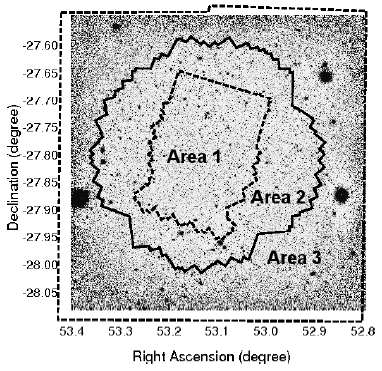
Figure 1.— Major areas defined in ECDFS. Background is the negative $J+K_{s}$ image from TENIS. The inner dashed line encloses the CANDELS/GOODS-S area (“Area 1”), the solid line encloses the deep X-ray coverage (CDFS, “Area 2”), and the outer dashed line (ECDFS) shows the MUSYC (Cardamone et al., 2010) coverage (“Area 3”) that defines the full area used in this paper.

The area centered on the GOODS-S field has been observed repeatedly with a large variety of facilities and instruments. As a result, numerous datasets with different bands and depths are available depending on the exact location. Reliable X-ray-to-optical associations and photometric redshifts can be obtained only when the data are homogeneous, and for this reason we split the area into subregions where the data are uniform. Three main regions share the same sets of data: Area 1 ($\sim$176 arcmin²) is the region covered by CANDELS and GOODS-S, Area 2 ($\sim$ 290 arcmin²) is the outer CDFS region surrounding CANDELS/GOODS-S, and Area 3 ($\sim$ 435 arcmin²) is the ECDFS region outside the CDFS. Figure 1 shows the three regions.

2.1. Photometric data from UV to MIR

Altogether the ECDFS has been covered by 50 bands from ultraviolet (UV) to mid-infrared (MIR) as listed in Table 1. Table 2 summarizes the catalogs used in each area.

Table 1Photometric Data

Filter	$\lambda_{\mathrm{eff}}$	FWHM	$5\sigma$ Limiting Depth	Instrument	Area
	(Å)	(Å)	(AB mag)	Telescope
$U$-CTIO	3734	387	26.63	Blanco/Mosaic-II	1
$U$-VIMOS	3722	297	27.97	VLT/VIMOS	1
F435W	4317	920	28.95/30.55	HST/ACS	1
F606W	5918	2324	29.35/31.05	HST/ACS	1
F775W	7693	1511	28.55/30.85	HST/ACS	1
F814W	8047	1826	28.84	HST/ACS	1
F850LP	9055	1236	28.55/30.25	HST/ACS	1
F098M	9851	1696	28.77	HST/WFC3	1
F105W	10550	2916	27.45/28.45/29.45	HST/WFC3	1
F125W	12486	3005	27.66/28.34/29.78	HST/WFC3	1
F140W	13635	3947	26.89/29.84	HST/WFC3	1
F160W	15370	2874	27.36/28.16/29.74	HST/WFC3	1
$Ks$-ISAAC	21605	2746	25.09	VLT/ISAAC	1
$Ks$-HAWKI	21463	3250	26.45	VLT/HAWK-I	1
$3.6\mu\mathrm{m}$-SEDS	35508	7432	26.52	Spitzer/IRAC	1
$4.5\mu\mathrm{m}$-SEDS	44960	10097	26.25	Spitzer/IRAC	1
$5.8\mu\mathrm{m}$-GOODS	57245	13912	23.75	Spitzer/IRAC	1
$8.0\mu\mathrm{m}$-GOODS	78840	28312	23.72	Spitzer/IRAC	1
$3.6\mu\mathrm{m}$-SIMPLE	35508	7432	23.89	Spitzer/IRAC	2, 3
$4.5\mu\mathrm{m}$-SIMPLE	44960	10097	23.75	Spitzer/IRAC	2, 3
$5.8\mu\mathrm{m}$-SIMPLE	57245	13912	22.42	Spitzer/IRAC	2, 3
$8.0\mu\mathrm{m}$-SIMPLE	78840	28312	22.50	Spitzer/IRAC	2, 3
$U38$	3706	357	25.33	WFI/ESO MPG	2, 3
$U$	3528	625	25.86	ESO MPG/WFI	2, 3
$B$	4554	915	26.45	ESO MPG/WFI	2, 3
$V$	5343	900	26.27	ESO MPG/WFI	2, 3
$R$	6411	1602	26.37	ESO MPG/WFI	2, 3
$I$	8554	1504	24.30	ESO MPG/WF	2, 3
$z$	8989	1285	23.69	Blanco/Mosaic-II	2, 3
$J$	12395	1620	22.44	Blanco/ISPI	2, 3
$H$	16154	2950	22.46	ESO NTT/SofI	2, 3
$K$	21142	3312	21.98	Blanco/ISPI	2, 3
$J$	12481	1588	24.50	CFHT/WIRCam	2, 3
$Ks$	21338	3270	23.90	CFHT/WIRCam	2, 3
FUV	1543	228	25.69	GALEX	1, 2, 3
NUV	2278	796	25.99	GALEX	1, 2, 3
IA427	4253	210	25.01	Subaru	1, 2, 3
IA445	4445	204	25.18	Subaru	1, 2, 3
IA464	4631	216	24.38	Subaru	1, 2, 3
IA484	4843	230	26.22	Subaru	1, 2, 3
IA505	5059	234	25.29	Subaru	1, 2, 3
IA527	5256	243	26.18	Subaru	1, 2, 3
IA550	5492	276	25.45	Subaru	1, 2, 3
IA574	5760	276	25.16	Subaru	1, 2, 3
IA598	6003	297	26.05	Subaru	1, 2, 3
IA624	6227	300	25.91	Subaru	1, 2, 3
IA651	6491	324	26.14	Subaru	1, 2, 3
IA679	6778	339	26.02	Subaru	1, 2, 3
IA709	7070	321	24.52	Subaru	1, 2, 3
IA738	7356	324	25.93	Subaru	1, 2, 3
IA768	7676	366	24.92	Subaru	1, 2, 3
IA797	7962	354	24.69	Subaru	1, 2, 3
IA827	8243	339	23.60	Subaru	1, 2, 3
IA856	8562	324	24.41	Subaru	1, 2, 3

1. Area 1: In this region, we primarily used the CANDELS-TFIT multi-wavelength catalog of Guo et al. (2013, hereafter G13), which covers the CANDELS GOODS-S area with 18 broad-band filters mostly from space observatories. The photometry was based on template-fitting (TFIT; Laidler et al., 2007), using the high resolution WFC3/$H$-band image to detect sources and define apertures, which were then used for photometry in lower-resolution images. TFIT was also applied to the MIR data from the Spitzer Extended Deep Survey (SEDS; Ashby et al., 2013). This deblending yields more accurate photo-z and also increases the probability of making correct X-ray to IR associations (see Section 3). In addition, the Area 1 data include 18 IBs at optical wavelengths provided by the MUSYC team (Cardamone et al., 2010). CANDELS collaborators (Donley et al. in preparation) have produced an IB-TFIT catalog with the same parameters used by G13. Despite being up to 2 magnitudes shallower than the rest of the optical data, the IB data are useful to identify emission lines, which can modify the choice of template best fitting the data and thus the photo-z (see Section 6.3). To these 36 bands we also added the near-UV (NUV) and far-UV (FUV) data from GALEX Data Release 6 and 7. The association between GALEX data and the WFC3/$H$-band catalog was done via positional matching within a radius of 1″. About 5% of all sources and $\sim$25% of X-ray-detected sources have UV counterparts. The combined data, which we refer to as “$\rm{TFIT}_{\rm{CANDELS+IB}}$”, have 34930 sources with up to 38 bands for computing photo-z.

2. Areas 2+3: These areas differ in depth of X-ray coverage (Section 2.2) but have the same data sets otherwise. For the CDFS and ECDFS surrounding Area 1, we merged the following photometric catalogs via coordinate cross match, allowing a maximum separation of 1″: (1) GALEX catalog (as above), (2) the original MUSYC catalog (Cardamone et al., 2010), and (3) the $J$ and $K_{s}$-band data from the Taiwan ECDFS Near-Infrared Survey (TENIS; Hsieh et al., 2012). Although TENIS is no deeper than existing NIR data, the TENIS data are more homogeneous over the entire field and have slightly different transmission curves, increasing the wavelength coverage. The MIR data for Area 2 and 3 came from the Spitzer IRAC/MUSYC Public Legacy in ECDFS (SIMPLE; Damen et al., 2011). These data are shallower than the SEDS data available in Area 1. Table 1 lists the data sets used, and we refer to this dataset as “MUSYC+TENIS”. There are 70049 sources in this photometry.

2.2. X-ray data

The X-ray catalogs to cross-match were obtained from the Chandra survey of 4Ms-CDFS observations covering Area 1+2 and from the 250ks-ECDFS observations covering Area 3. Two independent groups (Xue et al., 2011; Rangel et al., 2013) have provided source catalogs for 4Ms-CDFS using different methods for data reduction and source detection. Similarly for Area 3, both Lehmer et al. (2005) and Virani et al. (2006) have released X-ray source catalogs for the 250ks-ECDFS survey. We have cross-matched X-ray sources from both catalogs in each area.

For Areas 1+2 we used:

a. The 4Ms-CDFS source catalog of Xue et al. (2011) (hereafter X11) with 740 point-like X-ray sources. The sensitivity limits of the X-ray data are $3.2\times 10^{-17}$, $9.1\times 10^{-18}$, and $5.5\times 10^{-17}$ erg cm^-2 s^-1 for the full (0.5–8 keV), soft (0.5–2 keV), and hard (2–8 keV) bands, respectively.

b. The 4Ms-CDFS source catalog of Rangel et al. (2013) (hereafter R13) produced using the analysis methodology of Laird et al. (2009). The catalog contains 569 point-like X-ray sources and has sensitivity limits $4.2\times 10^{-17}$, $1.2\times 10^{-17}$, and $8.8\times 10^{-17}$ erg cm^-2 s^-1 in the full, soft, and hard bands, respectively.

For Area 3 we used:

c. The 250ks-ECDFS X-ray catalog from Lehmer et al. (2005) (hereafter L05) with 762 sources in the entire ECDFS of which 457 are in Area 3 (i.e., outside the 4Ms-CDFS area). Catalog sensitivity limits are $1.1\times 10^{-16}$ erg cm^-2 s^-1 in the soft (0.5–2 keV) band and $6.7\times 10^{-16}$ in the hard (2–8 keV) band.

d. The 250ks-ECDFS X-ray catalog from Virani et al. (2006) (hereafter V06) with 651 sources in the entire ECDFS of which 404 are in Area 3. Sensitivity limits are $1.7\times 10^{-16}$ and $3.9\times 10^{-16}$ erg cm^-2 s^-1 in the soft and hard bands, respectively.

2.3. Spectroscopic Data

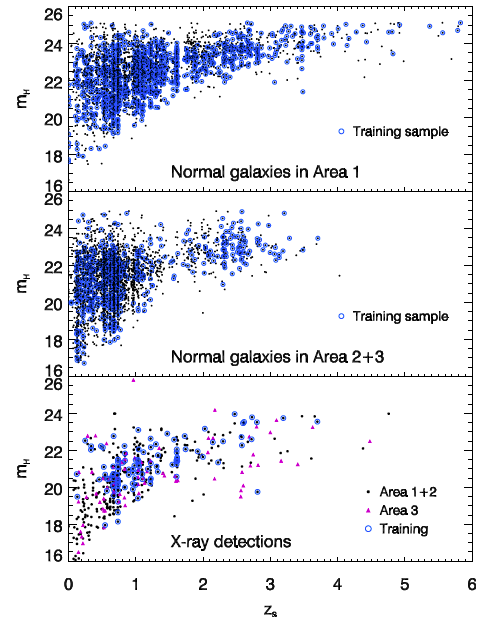
Figure 2.— $H$-band magnitude as a function of spec-z for all objects with spectroscopic redshifts. Black dots in the top panel represent normal galaxies in Area 1, where $\rm{TFIT}_{\rm{CANDELS+IB}}$ data are available. The middle panel shows normal galaxies identified from the MUSYC catalog in Areas 2 and 3. Black dots in the bottom panel represent X-ray-detected sources in Areas 1 and 2, and magenta triangles denote sources detected in the shallower X-ray data in Area 3. Open blue circles in all three panels indicate objects used for training.

The availability of spec-z for a subgroup of sources is essential for computing reliable photo-z via SED fitting (Dahlen et al., 2013). A subset of spec-z can first be used for training under the assumption that they are representative of the entire population. A different subset can then be used for testing photo-z quality. For this work we cross matched the photometric catalogs to a compilation of spec-z (N. Hathi, private communication), allowing a maximum separation of 1″. There are 2314 ($\sim$7%) Area 1 sources that have reliable spec-z and 3880 ($\sim 6\%$) such sources in Areas 2 and 3 (2016 in Area 2, 1864 in Area 3).

As discussed by Dahlen et al. (2013), optimal results are obtained when the templates used for the photo-z computation are calibrated on the photometry available for the spectroscopic training samples. For this reason the training samples should fully span the entire magnitude–redshift parameter space. Figure 2 shows that the 1000 sources randomly selected as our training samples are indeed spread over all redshift and magnitude ranges in the respective Areas. Because the photometry available in Area 1 differs from that in Area 2+3, two sets of training samples and computations of the zero-point offsets were used.

For the X-ray sources, we forgo using the training sample for computing zero-point offsets and instead use it to sample the AGN population and help build the AGN-galaxy hybrid templates needed for proper SED fitting and photo-z measurement (Salvato et al., 2009). For this purpose, we randomly chose $\sim$25% of the 4Ms-CDFS detections with available spec-z over the entire range of redshift and magnitude that have CANDELS data and used them as the training set to build hybrid templates. The remaining $\sim$75% were used for unbiased testing of the results. Details are given in the Appendix.

Table 2Catalogs used for redshift estimation and counterpart identification.

	Area 1	Area 2	Area 3
	4Ms-CDFS-X11	4Ms-CDFS-X11	250ks-ECDFS-L05
	4Ms-CDFS-R13	4Ms-CDFS-R13	250ks-ECDFS-V06
Cross	CANDELS-TFIT	MUSYC	MUSYC
matching	MUSYC	TENIS	TENIS
	TENIS	SIMPLE-IRAC	SIMPLE-IRAC
	SEDS-IRAC
Photo-z	CANDELS-TFIT	MUSYC	MUSYC
	IB-TFIT	TENIS	TENIS
	GALEX-UV	GALEX-UV	GALEX-UV
$N_{\mathrm{spz}}$	2314	2016	1864

3. X-ray to optical/NIR/MIR Associations

X-ray source positions can differ between catalogs because of different methods adopted for data reduction and source detection. The goal of this paper is not to judge which method of X-ray source detection is superior but rather to provide accurate photo-z for optical/NIR/MIR sources associated with X-ray sources. Associations between X-ray sources and possible counterparts were therefore done independently for each of the four X-ray catalogs (Sec 2.2), and duplicate sources were removed only at the end of the process as described below.

3.1. Comparing X-ray Catalogs

1. In Areas 1+2:

The major difference between the R13 and X11 catalogs is that R13 adopted a higher threshold for source detection. Despite that, there are some sources in the R13 catalog but not in X11. There are also astrometric differences, which can affect the association to an optical/NIR/MIR counterpart. Thus the redshift assigned to the X-ray source and also to the supposed counterparts can be different because different template libraries and priors were used for X-ray galaxies than for normal ones. In order to match X-ray catalogs, we shifted the X11 positions by $-0\farcs 175$ in R.A. and $0\farcs 284$ in Dec. to register them to the optical frame (Giavalisco et al., 2004). The R13 catalog is already on the MUSYC optical frame and was not shifted.

After astrometric shifting, we matched the X11 and R13 catalog coordinates, allowing a maximum distance of 10″. There are 545 sources in common with a maximum offset $<6\arcsec$ as shown in Figure 3. For these 545 sources, neither catalog has any additional X-ray source within 10″. As expected, all of the large offsets are for sources at large off-axis angles. For off-axis angles $<6\arcmin$, the median coordinate offset is 0$\farcs$13, and except for one source, the maximum offset at any off-axis angle is $<3\farcs 5$. We treat each of the 545 matched sources as a single X-ray detection. $54\%$ of these sources have a distance from each other larger than the positional error claimed for either of the catalogs. In addition, there are 195 sources detected by X11 but not R13 and 24 sources detected by R13 but not X11 for a total of 764 X-ray sources in Areas 1+2. As R13 mentioned, the unique sources to either of the two catalogs are mostly low-significance detections and therefore of lower reliability. In the following discussions, “X-” sources indicate those from X11 and “R-” those from R13.

2. In Area 3:

We adopted the Cardamone et al. (2008) astrometric calibration to align the V06 positions to the MUSYC and L05 catalogs, which were already in agreement. After the shift, the two catalogs have 366 source matches with offsets $<6\arcsec$. These have a median separation of 0$\farcs$16 (Fig. 4). We consider these 366 sources as the same X-ray detection. $12\%$ of these sources have a separation that is larger than the positional error associated with either of the catalogs. In addition, there are 91 sources in the L05 catalog but not V06 and 38 sources in the V06 catalog but not L05 for a total of 495 X-ray sources in Area 3. A compilation of the four X-ray catalogs with their original positions and fluxes is available under [Surveys] $>$ [CDFS] through the portal http://www.mpe.mpg.de/XraySurveys.

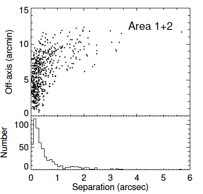
Figure 3.— Coordinate differences between X11 and R13 X-ray catalogs. The lower panel shows a histogram of offsets for the 545 sources Area 1 and 2 in common in the two catalogs. The upper panel shows the off-axis angle from the Chandra aim point as a function of the angular offset.

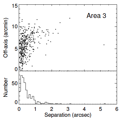
Figure 4.— Coordinate differences between L05 and V06 X-ray catalogs. The lower panel shows a histogram of offsets for the 495 sources in Area 3 in common in the two catalogs. The upper panel shows the off-axis angle from the Chandra aim point as a function of the angular offset.

3.2. Matching method

We used a new association method based on Bayesian statistics which allows pairing of sources from more than two catalogs at once while also making use of priors. Salvato et al. (2014, in preparation) will give details, but in brief the code finds matches based on the equations developed by Budavári & Szalay (2008). Then additional probability terms based on the magnitude and color distributions are applied. (See Naylor et al. 2013 for a similar approach.) The code was developed in view of the launch of eROSITA (Merloni et al., 2012), where an expected million sources will be scattered over the entire sky and will have a non-negligible positional error and/or non-homogenous multi-wavelength coverage, conditions not optimal for association methods like Maximum Likelihood (e.g., Brusa et al. 2007; Luo et al. 2010; Civano et al. 2012). The new method provides the same quality of results as Maximum Likelihood in a much shorter time because matches are done simultaneously across all bands. Thus for example sources that are extremely faint or undetected in optical bands but brighter in the IRAC 3.6 $\mu\mathrm{m}$ band can be identified as counterparts in a single iteration.

For the 4Ms-CDFS sources (X11 and R13) located in Area 1, we used the CANDELS/$H$-selected catalog, TENIS/$J\&K_{s}$-selected catalog, MUSYC/$BVR$-selected catalog, and the deblended SEDS/IRAC 3.6 µm catalog. For the 4Ms-CDFS sources located in Area 2, we matched the X-ray sources to the TENIS/$J\&K_{s}$-selected catalog, MUSYC/$BVR$-selected catalog, and SIMPLE/IRAC 3.6$\mu\mathrm{m}$ catalog. The same set of these three catalogs was also used in Area 3 for finding the associations for the 250ks-ECDFS sources (L05 and V06). Table 2 summarizes the catalogs matched in each Area.

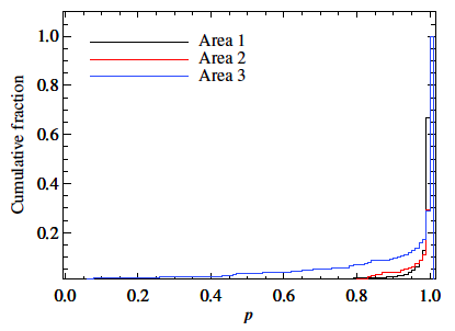
Figure 5.— Cumulative fraction of the posterior $p$ for the possible counterparts to the X-ray sources in Area 1, 2, and 3 as indicated in the legend.

For each X-ray source (740 from X11, 569 from R13, 440 from L05, and 374 from V06), we considered all catalog objects lying within 4″ of the X-ray position and computed the posterior probability $p$ that the given object is the correct counterpart. Figure 5 shows the distribution of the posteriors for all the possible associations in the three areas. In Area 1 where the data are deeper and better resolved, more than $98\%$ of the X-ray sources have at least one association with $p>0.7$, and we consider this $p$ value the threshold for defining an association in all three areas. Area 3 has a distribution of $p$ that reaches lower values, but because of the shallowness and lower resolution of the data, we consider not reliable the association with $p<0.7$. Our catalogs (see Sec. 7) include the $p$ value to allow users to define a stricter threshold, depending on the scientific use intended.

Figure 6 shows examples of ambiguous identifications. In all three cases shown, a single X-ray source has two possible $H$-band associations with $p>0.99$. Even the simultaneous use of deblended IRAC photometry from SEDS does not help in associating a unique counterpart. The example in the middle shows that despite the high resolution of the CANDELS images, the upper source is still blended, and probably a third component is present. If a further deblending were applied, the $H$ flux would be split among multiple components, thus reducing the probability of the upper source being the right association. In practice, we attempted no further deblending and simply flagged these kinds of objects as sources with multiple counterparts. For these cases, in addition to the photo-z computed using normal galaxy templates, we also provide the values obtained by assuming that they are AGNs. The photo-z results reveal that $\sim 20\%$ of these close pairs have similar redshifts and may be associated with galaxy mergers or galaxy groups. However the majority of apparent pairs are projections of unrelated objects.

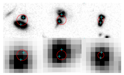
Figure 6.— Three examples of multiple $H$-band associations (from left to right X-115, X-517, and X-224) in $H$-band (upper) and IRAC-3.6$\mu\mathrm{m}$ (lower). The size of each cutout is $5^{\prime\prime}\times 5^{\prime\prime}$ . The red circles are centered at the X-ray position with radius corresponding to the positional error. The cyan crosses indicate the positions of $H$-band detected sources from G13. These three cases have two $H$-band associations both with probabilities greater then 0.99. The uses of deblended IRAC photometry does not help in making a unique secure association.

3.3. Matching results

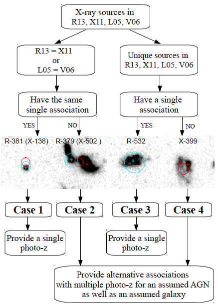
Figure 7.— Flow chart of the process for four cases of X-ray to optical/NIR/MIR associations. $H$-band negative images ($5^{\prime\prime}\times 5^{\prime\prime}$) are provided as examples for each case . Dashed-line circles show the X11 (red) and R13 (cyan) X-ray positions and positional uncertainties. Red and cyan crosses show the corresponding $H$-band counterparts.

Figure 7 shows the decision tree for X-ray source associations and computing photo-z, and Table 3 gives numbers for each case in each Area. There are four cases:

1. Case 1: An X-ray source in both catalogs with one optical/NIR/MIR association. Case 1 means the same unique association was chosen even though the X-ray catalog positions may differ between X11 and R13 or between L05 and V06. There are 714 of these sources in Areas 1+2+3.

2. Case 2: An X-ray source in both catalogs with differing optical/NIR/MIR associations. Case 2 can arise from two causes: (1) position differences in the X-ray catalogs may point to different counterparts, or (2) there may be more than one potential counterpart near the X-ray position(s), and we cannot tell which is the right one. Some of the latter may be blended sources with more than one galaxy contributing to the X-ray flux. In total, there are 181 case 2 sources in Areas 1+2+3. These sources are identified in the final catalogs, and counterpart photo-z are calculated using both AGN and normal galaxy SED templates (see Section 7) .

3. Case 3: X-ray sources found in one catalog but not the other, having a unique counterpart. There are 235 of these sources in Areas 1+2+3.

4. Case 4: X-ray sources found in only one catalog and having multiple possible counterparts. There are 77 such sources in Areas 1+2+3. As for Case 2, the catalogs identify all the possible counterparts and provide both AGN and normal galaxy photo-z results for each.

In summary, 1207 out of 1259 ($\sim$96%) of the X-ray sources are associated with multi-wavelength counterparts, and 258 of them ($\sim$21%) have multiple counterparts possible. There are 26 sources for which the counterpart is detected only in the IRAC bands, and no photo-z computation is possible for these. All the other sources have at least six photometric points, and a photo-z is provided. The photo-z catalog (see Sec. 7) entry for each source indicates the number of photometric points used for the photo-z computation. The remaining 52 sources ($\sim 4\%$) either have no identifications in any of the optical/NIR/MIR catalogs ($\sim 1\%$) or have possible counterparts identified with $p<0.7$ ($\sim 3\%$). For these sources, the photo-z are not available as well.

Table 3Results of X-ray to optical/NIR/MIR associations in ECDFS .

	$N_{x}$	Case1	Case2	Case3	Case4	$N_{ctp}^{single}$	$N_{ctp}^{multi}$	$N_{ctp}$	$N_{ctp}^{multi}/N_{ctp}$	$N_{ctp}/N_{x}$
Area 1	509	272	67	130	29	402	96	498	19%	$98\%$
Area 2	255	170	29	35	12	205	41	246	17%	$96\%$
Area 3	495	272	85	70	36	342	121	463	26%	$94\%$
TOTAL	1259	714	181	235	77	949	258	1207	21%	$96\%$

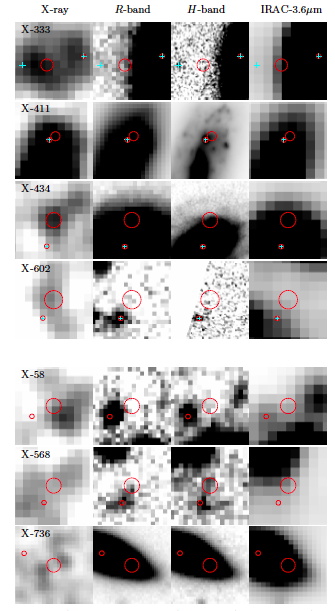
Figure 8.— Multi-wavelength images of the seven sources from X11 for which we found new, secure ($p>0.9$) counterparts. Wavelengths are indicated above each set of panels. The four sources in the upper group are in Area 1 and have CANDELS $H$-band images. The three sources in the lower group have no WFC3-$H$, and TENIS-$K_{s}$ is shown instead. X-ray images are full-band from X11. The red dashed circles are centered at the X11 positions with their radii showing the corresponding positional uncertainty. Cyan crosses in the upper panels show all $H$-band detections, and the solid red circles show the catalog position of the chosen counterpart. All cutouts are $5^{\prime\prime}\times 5^{\prime\prime}$ except that X-736 is $10^{\prime\prime}\times 10^{\prime\prime}$.

3.4. Comparison to previous results in Area 1+2

X11 used likelihood ratio matching to assign counterparts to 716 out of 740 X-ray sources in Areas 1+2. Our code and the newly available ancillary data give secure counterparts (with $p>0.9$) for seven additional sources shown in Figure 8. Most of the new counterparts are offset from the X-ray position by 1–2 times the X-ray position uncertainty. The most likely reason for finding new identifications is having better imaging data available, but there remains a chance some of the X-ray sources are not real.

Figure 9 shows an example of a revised X-ray association. In this case low resolution catalogs give a single counterpart for the source (R-57=X-234) for either X-ray position However, the high-resolution WFC3/$H$-band image reveals at least four sources close together, and the slightly different coordinates provided by X11 and R13 point to different but equally likely counterparts. This difference is mainly due to the catalogs chosen for cross matching rather than the matching method. The Bayesian method should in principle give the same result as the maximum likelihood method, but the ability to match several catalogs simultaneously greatly improves the efficiency of the matching.

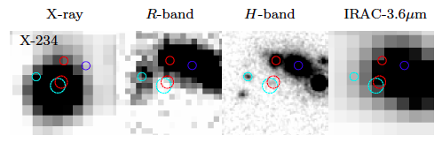
Figure 9.— Negative images of the source R-57 (=X-234). Image wavelengths are indicated at the top, and each image is $5^{\prime\prime}\times 5^{\prime\prime}$. Red dashed-line circles are centered at the position provided by X11 and cyan dashed-line circles at the position given by R13. Circle sizes indicate the respective X-ray position uncertainties. Red and cyan solid-line circles are the counterparts we assign to the two X-ray positions, and the blue circle indicates the counterpart assigned by X11.

4. Photo-z for Non X-ray detected Galaxies

This section focusses on the X-ray-undetected sources, which we refer to as “normal galaxies” even though some will in fact be AGNs. The derived photo-z will be reliable to the extent of the “normal galaxies” which have normal galaxy SEDs at observed visible/infrared wavelengths. X-ray sources need more tuning for accurate photo-z and are discussed in Section 5.

The photo-z were computed using LePhare (Arnouts et al., 1999; Ilbert et al., 2006), which is based on a $\chi^{2}$ template-fitting method. For the normal galaxies, we adopted the same templates, extinction laws, and absolute magnitude priors as Ilbert et al. (2009). In short, 31 stellar population templates were corrected for theoretical emission lines by modeling the fluxes with line ratios of [O III]/[O II], H$\beta$/[O II], H$\alpha$/[O II], and Ly$\alpha$/[O II]. In addition to the galaxy templates, we also included a complete library of star templates as did Ilbert et al. (2009) and Salvato et al. (2009). Four extinction laws (those of Prevot et al. 1984, Calzetti et al. 2000, and two modifications of the latter, depending on the kind of templates) were used with $E(B-V)$ values of 0.00 to 0.50 in steps of 0.05 mag. Photo-z values were allowed to reach $z=7$ (in steps of 0.01) because deeper photometry allows us to reach higher redshifts (see details given by Ilbert et al. 2009). The fitting procedure included a magnitude prior, forcing sources to have an absolute magnitude in rest $B$-band between $-8$ and $-24$. Photometric zero-point corrections were incorporated but never exceeded 0.1 mag. Final best parameters came from minimizing $\chi^{2}$. We advise against this step for the AGNs because optical variability is intrinsic to the source and not accounted for in the photometry.

All the normal galaxies were selected from either the CANDELS-TFIT catalog or the MUSYC catalog (Sec. 2.1). Photo-z are based on $\rm{TFIT}_{\rm{CANDELS+IB}}$ photometry for sources detected in the CANDELS-TFIT catalog and otherwise on MUSYC+TENIS photometry. The majority of normal galaxies have $\rm{TFIT}_{\rm{CANDELS+IB}}$ photometry in Area 1 but only MUSCY+TENIS photometry in Areas 2+3.

Quantifying the photo-z accuracy ($\sigma_{\mathrm{NMAD}}$), the percentage of the outliers ($\eta$), and the mean offset between photo-z and spec-z ($\mathrm{bias}_{z})$ was based on the spectroscopic samples. Table 4 gives these measures of photo-z quality for the global samples and for subsamples split into magnitude and redshift bins.

4.1. Area 1

The overall outlier fraction of $\sim$3.8% in this region is comparable to the most recent work by the CANDELS team (Dahlen et al., 2013). However, the deblended IB photometry from MUSYC improves the accuracy to $\sigma_{\mathrm{NMAD}}=0.012$ (from $\sigma_{\mathrm{NMAD}}=0.026$ by Dahlen et al. 2013) and $\mathrm{bias}_{z}=-0.001$ (from $\mathrm{bias}_{z}=-0.005$). Figure 10 illustrates the results. Outlier fractions and scatter are larger for the fainter galaxies (Table 4), but bias is only a weak function of source magnitude. Bias is, however, larger for $z>1.5$ galaxies than for those at lower redshifts. Scatter and outlier fraction are also larger at $z>1.5$, but this mostly reflects the typically fainter magnitudes of the more distant sources.

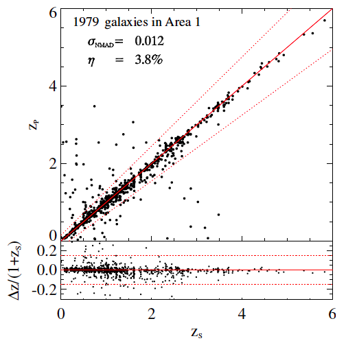
Figure 10.— Upper panel: Photo-z vs spec-z. Dots represent all normal galaxies with spec-z in Area 1. The solid line represents $z_{{p}}=z_{{s}}$; the dotted lines represent $z_{{p}}=z_{{s}}\pm 0.15(1+z_{{s}})$. Lower panel: Same but plotted as the difference $\Delta z\equiv(z_{{p}}-z_{{s}})$.

The decreased outlier fraction in the present survey requires both the deeper CANDELS-TFIT data and the deblended IB photometry. Table 5 gives data quality measures for 1541 sources in common using various data sets. Using only MUSYC+TENIS, but not the deep $\rm{TFIT}_{\rm{CANDELS+IB}}$ data, produces the same data quality as Cardamone et al. (2010) as expected. However using the $\rm{TFIT}_{\rm{CANDELS+IB}}$ photometry decreases the outlier fraction from $\sim$4% to $\sim$2%, and the decrease is most substantial (more than a factor of two) for the faint and distant sources. (See Table 5.) Figure 11 illustrates the comparison and in particular the decrease in outliers at $z_{s}>2$. The difference comes from the use of deep space-based data (i.e., CANDELS) and the TFIT technique for deblending the lower-resolution bands. However, the IB data are also important. Dahlen et al. (2013) used the CANDELS-TFIT data, while their results (included in Table 5) are better than with the ground-based data alone, they are not as good as with the combined data sets (i.e., $\rm{TFIT}_{\rm{CANDELS+IB}}$). Adding the IB data improves results—mainly in accuracy but also in outlier fraction—even for the fainter subset of the sample.

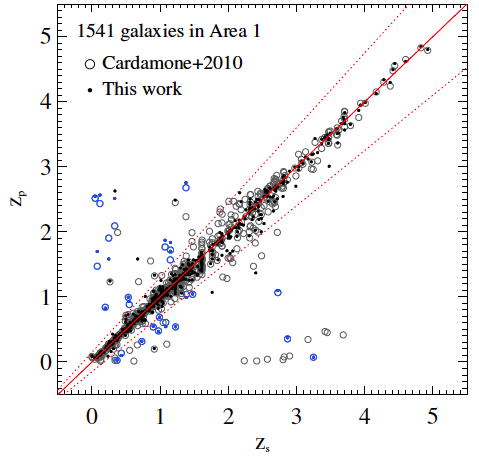
Figure 11.— Photo-z vs. spec-z for 1541 normal galaxies in Area 1. Black dots are results from this work, and grey open circles are results from Cardamone et al. (2010). Blue dots and blue open circles indicate objects that are outliers both in our work and in that of Cardamone et al. (2010).

Table 4Photo-z Quality for Normal Galaxies

	Area 1				Area 2+3				Area 1+2+3
	$N$	$\mathrm{bias}_{z}$	$\sigma_{\mathrm{NMAD}}$	$\eta(\%)$	$N$	$\mathrm{bias}_{z}$	$\sigma_{\mathrm{NMAD}}$	$\eta(\%)$	$N$	$bias_{z}$	$\sigma_{\mathrm{NMAD}}$	$\eta(\%)$
Total	1979	-0.001	0.012	3.79	3444	0.001	0.009	4.21	5423	0.001	0.010	4.06
$R<23$	576	0.003	0.008	1.04	2414	0.001	0.009	2.20	2990	0.001	0.009	1.97
$R>23$	1403	-0.002	0.015	4.92	1030	0.002	0.012	8.93	2433	-0.001	0.013	6.62
$H<23$	1323	-0.000	0.011	2.87	2428	0.002	0.009	2.72	3751	0.001	0.009	2.77
$H>23$	656	-0.002	0.016	5.64	1016	-0.001	0.011	7.78	1672	-0.001	0.012	6.9
$z<1.5$	1652	0.002	0.011	3.51	3316	0.002	0.009	3.89	4968	0.002	0.009	3.76
$z>1.5$	327	-0.013	0.021	5.20	128	-0.008	0.031	12.50	455	-0.011	0.024	7.25

Table 5Comparison of Photo-z Results for Normal Galaxies in Area 1

		$\rm{TFIT}_{\rm{CANDELS+IB}}$			MUSYC+TENIS			Cardamone+2010			Dahlen+2013
	$N$	$\mathrm{bias}_{z}$	$\sigma_{\mathrm{NMAD}}$	$\eta(\%)$	$\mathrm{bias}_{z}$	$\sigma_{\mathrm{NMAD}}$	$\eta(\%)$	$\mathrm{bias}_{z}$	$\sigma_{\mathrm{NMAD}}$	$\eta(\%)$	$\mathrm{bias}_{z}$	$\sigma_{\mathrm{NMAD}}$	$\eta(\%)$
Total	1541	0.000	0.011	2.14	0.003	0.012	3.96	0.000	0.011	3.96	-0.005	0.026	2.47
$R<23$	506	0.003	0.009	0.79	0.002	0.008	0.79	0.002	0.008	0.99	-0.002	0.026	0.99
$R>23$	1035	-0.002	0.013	2.80	0.003	0.016	5.51	-0.001	0.016	5.41	-0.006	0.026	3.19
$H<23$	1064	0.001	0.010	1.60	0.003	0.010	2.07	0.000	0.010	2.07	-0.006	0.027	1.97
$H>23$	477	-0.002	0.014	3.35	0.002	0.021	8.18	0.000	0.022	8.18	-0.001	0.024	3.56
$z<1.5$	1308	0.002	0.010	2.14	0.004	0.011	3.13	0.002	0.010	2.98	-0.005	0.026	2.45
$z>1.5$	233	-0.014	0.019	2.15	-0.002	0.030	8.58	-0.008	0.045	9.44	-0.002	0.023	2.58

4.2. Areas 2 and 3

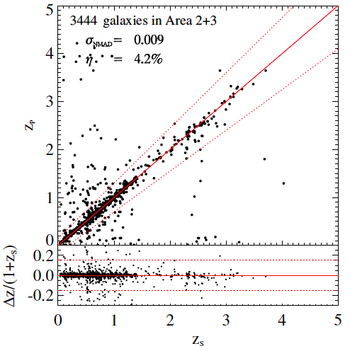
Figure 12.— Photo-z vs spec-z of normal galaxies in Areas 2+3.

.

Outside the CANDELS area, photo-z quality using MUSYC+TENIS photometry is similar to that of Cardamone et al. (2010). Figure 12 illustrates the results. The brighter and lower-redshift subsets have photo-z quality almost as good as in Area 1 (see Table 4), but fainter galaxies have a higher outlier fraction. This is just as expected from the tests in Section 4.1.

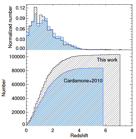
Figure 13.— Upper panel: normalized photo-z distribution for normal galaxies. Grey hatched area shows results of this work, and blue shaded area shows results of Cardamone et al. (2010)/ Lower panel: cumulative number of normal galaxy photo-z redshifts for this work and for Cardamone et al. (2010) as labeled.

The entire ECDFS (Areas 1+2+3) contains $\sim 104000$ normal galaxies that have photo-z up to $z\sim 7$. Figure 13 shows the advantage of using WFC3 NIR to detect more sources in total and especially at $z\gtrsim 2$. An interesting paradox is that we actually have a slightly lower fraction of sources at $z>1.5$ than Cardamone et al. (2010). This is probably because their higher outlier fraction, lacking deep NIR data, leads to more outliers with apparent $z>1.5$.

5. Photo-z for X-ray sources

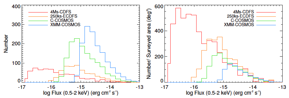
Figure 14.— Soft X-ray flux distributions in numbers (left) and source densities (right). Histograms show distributions for the 4Ms-CDFS (Areas 1 and  2), 250ks-ECDFS (Area 3), and comparison surveys Chandra-COSMOS (Elvis et al., 2009) and XMM-COSMOS (Cappelluti et al., 2009) surveys as indicated in the legend.

AGNs require special treatment to calculate photo-z. This paper uses deep X-ray data to identify candidate AGNs. However, X-ray surveys as deep as the 4Ms-CDFS also detect significant numbers of star-forming galaxies. The library must therefore include templates of normal galaxies, AGNs, and hybrids.

5.1. Template Library Methods

Luo et al. (2010) computed photo-z for sources in the 2Ms-CDFS by using the spectra of known sources as templates for SED fitting. Using the entire spectroscopic sample for template training gave an apparent accuracy $\sim$0.01 with almost no outliers. However, unbiased testing suggested a true accuracy of 0.059 and $\sim$9% outliers. This demonstrates how important the training sample is. For the same field, Cardamone et al. (2010) created hybrid templates by combining normal galaxy templates with the SED of a type 1 AGN. The method gave accurate results ($\sigma_{\rm NMAD}\sim 0.01$) but large outlier fraction ($\sim 12\%$). Salvato et al. (2009, 2011, hereafter S09, S11) pursued a different approach for X-ray sources in the COSMOS field (Scoville et al., 2007) detected by XMM (Cappelluti et al., 2009) and by Chandra (Elvis et al., 2009). This involved (1) correcting the photometry for variability when applicable; (2) separating the optical counterparts to the X-ray sources into two subgroups: point-like and/or variable sources in one and extended, constant sources in the other; (3) applying absolute magnitude priors to these two subgroups, assuming that the former are AGN-dominated while the latter are galaxy-dominated; (4) creating AGN-galaxy hybrids, using different libraries for the two subgroups. This same procedure substantially reduced the fraction of outliers and gave higher accuracy than standard photo-z techniques when applied to X-ray sources in COSMOS. The procedure has also yielded reliable results for the Lockman Hole (Fotopoulou et al., 2012) and AEGIS fields (Nandra et al. 2014, submitted). S11 also verified the need for depth-dependent template libraries by showing that hybrids defined for XMM-COSMOS are not optimal for the deeper Chandra-COSMOS. Even though the X-ray-faint Chandra sources are AGNs (i.e., $L_{\rm{x}}>10^{42}$), normal galaxy templates gave better results for them than AGN-dominated templates.

5.2. Constructing Population-dependent SED Libraries

For this work, we constructed new hybrid templates following the procedure of S09 and S11 (Sec. 5.1). First we point out that the difference of the X-ray flux distributions between the two X-ray surveys used in this work (i.e., 4Ms-CDFS and 250ks-ECDFS) is even more extreme than what we have found in S11 (i.e., XMM-COSMOS and Chandra-COSMOS).

Fig. 14 shows the soft X-ray flux distributions of the 4Ms and 250ks sources, together with the distributions from the Chandra-COSMOS (Elvis et al., 2009) and XMM-COSMOS (Cappelluti et al., 2009). The left panel shows the distribution in numbers for each survey. Because of the sky coverage and the depth of the observations, most of the 4Ms-CDFS sources are located in the faint part of the flux distribution, which is opposite to the locus occupied by the shallower observations (e.g. XMM-/Chandra-COSMOS and 250ks-ECDFS). After normalizing by the total surveyed area (see the right panel), it reveals that the X-ray bright sources which are similar to the XMM-COSMOS sources are very rare in the 4Ms survey. This implies that the library of hybrids used in XMM-COSMOS is probably not representative of the 4Ms population. Based on this considerations, we need to build a new library for the fainter 4Ms-CDFS population. The Appendix gives details, but in short AGN SEDs were combined in various proportions with semi-empirical galaxy SEDs (the same as already successfully used by Gabasch et al. (2004), Drory et al. (2005), and Feulner et al. (2005)) from the FORS Deep Field (Bender et al., 2001) to make hybrid templates. The AGN SEDs were modified QSO1 and QSO2 originally from Polletta et al. (2007). Separate libraries were used for (a) point-like sources in Areas 1+2, (b) point-like sources in Area 3, and (c) extended sources in all Areas. Because the flux distribution of point-like sources in Area 3 is similar to that of the XMM-COSMOS field, library (b) for point-like sources in that area was the same as used by Salvato et al. (2009).

As a first step, we split the sources into extended and point-like subgroups depending on the observed source FWHM in the WFC3/$H$-band images for Area 1 and the MUSYC/$BVR$ images for Areas 2 and 3. The extended sources were assumed to be host-dominated, and being seen as extended means they are likely to be at low redshift. For these sources, we applied an absolute magnitude prior $-24<M_{B}<-8$ and used templates with at most a small AGN fraction. Point-like sources are usually AGN-dominated and can be at any redshift. We therefore applied a prior $-30<M_{B}<-20$ to these and used hybrid AGN-galaxy templates. The library of stellar templates was the same as used by Ilbert et al. (2009) and Salvato et al. (2009).

For the XMM-COSMOS field, Salvato et al. (2009) had multi-wavelength, multi-epoch observations spanning several years. About 1/4 of sources seen in those were variable. The lack of multi-epoch data for the CDFS/ECDFS means that we cannot detect the variable objects and correct their photometry. However, these objects are a minor contributor to the X-ray population in the much smaller CDFS area (1/15 of XMM-COSMOS area). Therefore only a minor fraction of the Area 1 and 2 sources are likely to be variable. The major effect of being unable to correct for variability will be an increased outlier fraction rather than decreased photo-z accuracy (Salvato et al., 2009). Area 3, covered at 250 ks depth, is an intermediate case, and part of the photo-z inaccuracy there could be due to lack of variability correction. The spectroscopic testing in the respective Areas (Table 6) quantifies the outlier fractions and the inaccuracies resulting from all causes.

Table 6Photo-z Quality for X-ray Sources

	Area 1				Area 2				Area 3				Area 1+2+3
	$N$	$bias_{z}$	$\sigma_{\mathrm{NMAD}}$	$\eta(\%)$	$N$	$\mathrm{bias}_{z}$	$\sigma_{\mathrm{NMAD}}$	$\eta(\%)$	$N$	$\mathrm{bias}_{z}$	$\sigma_{\mathrm{NMAD}}$	$\eta(\%)$	$N$	$\mathrm{bias}_{z}$	$\sigma_{\mathrm{NMAD}}$	$\eta(\%)$
Total	300	-0.002	0.012	2.67	104	-0.002	0.014	6.73	148	-0.004	0.016	10.14	552	-0.002	0.014	5.43
$R<23$	171	-0.004	0.010	1.17	80	-0.000	0.014	5.00	109	0.001	0.013	8.26	360	-0.002	0.011	4.17
$R>23$	129	0.001	0.024	4.65	24	-0.008	0.016	12.50	39	-0.018	0.023	15.38	192	-0.004	0.023	7.81
$H<23$	278	-0.003	0.012	1.80	102	-0.002	0.014	6.86	69	-0.004	0.016	10.14	449	-0.003	0.013	4.23
$H>23$	22	0.012	0.014	13.64	2	-0.010	0.026	0.00	79	-0.004	0.016	10.13	103	-0.001	0.014	10.68
$z<1.5$	240	-0.001	0.012	2.50	86	-0.001	0.015	4.65	112	-0.003	0.020	8.04	438	-0.001	0.014	4.34
$z>1.5$	60	-0.004	0.014	3.33	18	-0.009	0.012	16.67	36	-0.009	0.010	16.67	114	-0.006	0.012	9.65

5.3. Results

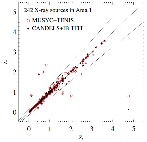
Figure 15.— Comparison of photo-z to spec-z with and without $\rm{TFIT}_{\rm{CANDELS+IB}}$ photometry. Filled points show results for 242 X-ray sources from the Cardamone et al. (2010) catalog using the full $\rm{TFIT}_{\rm{CANDELS+IB}}$ dataset. Open circles show results for the same sources using only the MUSYC+TENIS data.

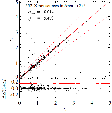
Figure 16.— Comparison of photo-z to spec-z for all X-ray sources in Areas 1+2+3.

In Area 1, where $\rm{TFIT}_{\rm{CANDELS+IB}}$ photometry and high-resolution space-based images are available, the photo-z for X-ray sources (Table 6) are as accurate as those for normal galaxies (Table 4). Remarkably, the outlier fraction is actually lower for the X-ray sources than for normal galaxies. Excellent photo-z quality is maintained even for $z>1.5$. Figure 15 shows that the results are largely attributable to the WFC3 data with their high angular resolution. Instead of using ground-based data (i.e., MUSYC+TENIS), the use of $\rm{TFIT}_{\rm{CANDELS+IB}}$ catalog allows us to reduce the outlier fraction by a factor of 3. The improvement is especially great for the $R>23$ and $z>1.5$ sources. The outlier fractions decreases from $6.3\%$ to $2.1\%$ for faint sources and from $12.8\%$ to $2.6\%$ for high-redshift sources. Comparison with Area 2 also confirms the importance of the WFC3 data. Without these data, photo-z accuracy deteriorates only slightly (Table 6), but the outlier fraction triples. Most of the outlier increase comes from the $R>23$ and $z>1.5$ subsets. (There are only two sources with $H>23$, and numerical results for that bin are meaningless.)

Area 3 has a larger fraction of outliers than either of the other two Areas, though accuracy for the non-outliers is little worse than in Areas 1 and 2 (Table 6). Three effects probably contribute to the larger fraction of outliers. One is shallower photometry at the border of the field (Fig. 1), leading to larger errors. Second, the X-ray coverage is shallower in the larger Area 3, thus the fraction of varying Type 1 AGN is presumably higher. The lack of variability correction will therefore have a larger effect. This is likely exacerbated by the third effect, having to use ground-based images rather than higher-resolution images for classifying sources as point-like or extended. In Area 1, about 30% of sources are classified point-like using WFC3 but extended on a ground-based image, due to the low resolution of the images and being sensitive to the presence of nearby sources. Using the template library for the extended sources rather than for point-like classification would have doubled the outlier fraction.

Furthermore, in order to identify possible outliers among the sources without spec-z, we look at the distribution of observed-frame X-ray luminosity as a function of redshift. In Figure 17, three sources with apparent extreme redshift are probably outliers. They are located on the edge of the optical images and have unreliable or non-existent MUSYC photometry, leaving only six photometric data points (from the TENIS catalog). Photo-z with so few data points cannot be trusted.

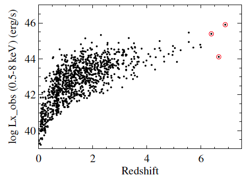
Figure 17.— Distribution of 0.5–8 keV observed-frame X-ray luminosity as a function of redshift for all X-ray sources. Redshifts are spec-z if available and otherwise photo-z. Red open circles indicate the three anomalous sources that have unreliable photo-z.

6. Discussion

6.1. Photometric Redshift Accuracy Beyond the Spectroscopic Limit

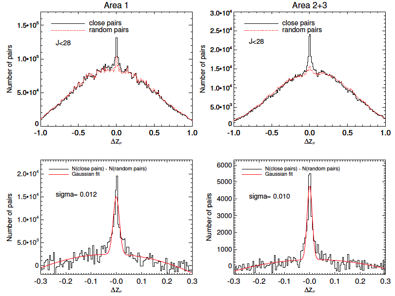
Figure 18.— Distributions of photo-z differences for pairs of galaxies. In the upper panels, red dotted lines represent differences for random pairs and black solid lines represent differences for pairs having angular separation $<$15″. Only galaxies with $J<28$ are included. The lower panels show results for close pairs after subtracting the distributions for random pairs. Black lines show the observed $\Delta z_{p}$, and red lines show a Gaussian fit with standard deviation sigma as indicated in each panel. The left two panels are for Area 1 and the right two for Areas 2+3.

Using spec-z to estimate photo-z accuracy (as in Tables 4 and 6) is not representative of sources fainter than the spectroscopic limit. Quadri & Williams (2010) introduced a method for estimating photo-z accuracy based on the tendency of galaxies to cluster in space. Because of clustering, galaxies seen close to each other on the sky have a significant probability of being physically associated and having the same redshift. Therefore the distribution of photo-z differences ($\Delta z_{{p}}$) of close pairs will show an excess at small redshift differences over the distribution for random pairs. This is seen in Figure 18. The excess for close pairs with magnitude $J<28$ fits a Gaussian with standard deviation $\sigma=0.012$ in Area 1 and $0.010$ in Areas 2+3. Because the width includes the scatter from both paired galaxies, the photo-z uncertainty for an individual object should be $\sigma/\sqrt{2}$. These values are given in Table 7. The pair test reveals that the faint sources without spec-z have photo-z accuracy similar to that of sources bright enough to have spectroscopic data.

Table 7Photo-z Scatter from Pair Statistics

	Area 1	Areas 2+3
$J<25$	0.008	0.007
$J<26$	0.009	0.007
$J<27$	0.009	0.007
$J<28$	0.008	0.007

6.2. The Impact of Intermediate-band Photometry

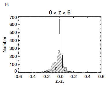
Figure 19.— Distribution of photo-z minus spec-z. Histograms show $z_{p}-z_{s}$ distribution for all galaxies with spec-z in Area 1. Black line shows results for photo-z with IB photometry included, and hatched area shows results for the same galaxies with IB data omitted.

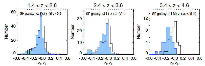
Figure 20.— Distribution of photo-z minus spec-z for star-forming galaxies selected by rest $BzK$ colors. Histograms show ($z_{\rm p}-z_{\rm s}$) distributions in various redshift bins as indicated above each panel. Black lines show the distributions for photo-z with IB photometry included, and blue areas show distributions for the same galaxies with IB photometry omitted. All data are from Area 1.

Previous work has shown the importance of IB photometry for photo-z, especially because IB data can show the presence or absence of emission lines in galaxy SEDs. For example Ilbert et al. (2009) showed that including IBs improved photo-z accuracy from 0.03 to 0.007 for normal galaxies with $i^{+}<22.5$ in the COSMOS field. Cardamone et al. (2010) found the same in the ECDFS. For AGNs, Salvato et al. (2009) showed that for both extended and point-like X-ray sources in COSMOS, accuracies and outlier fractions were substantially better when IBs were included.

In the current data, the IB photometry is much shallower than the NIR data from CANDELS (Table 1). To examine whether the shallow IB data are helpful or not in this case, we recomputed the Area 1 photo-z with exactly the same CANDELS-TFIT dataset (Guo et al., 2013) used by Dahlen et al. (2013), i.e., without IBs. Results are given in Table  5, and Figure 19 compares results with IBs and without.

Without the IBs, the outlier fraction is 5%, accuracy is 0.037, and $\mathrm{bias}_{z}=-0.010$. These are similar to the results of Dahlen et al. (2013) “method 11H,” which used the same code as this work. The negative value of $\mathrm{bias}_{z}$ indicates underestimation of photo-z on average. That results in lower galaxy luminosities and incorrect rest colors. As discussed by Rosario et al. (2013), these may lead to incorrect measurements of galaxy ages and stellar populations. The IB data improve the accuracy and mean offset substantially, creating a narrower and more symmetric peak of photo-z values around the spec-z (Fig. 19).

Intermediate bands should be most important for objects that have strong emission lines in their spectra. Strong emission lines can arise either from vigorous star formation or an AGN. To quantify the effect, we applied (inverse) $BzK$ selection (Daddi et al., 2004) to define a sample of star-forming objects among those with reliable spec-z. In order to extend the selection at high redshift, we applied the revised $BzK$ criterion as defined by Guo et al. (2013). Fig. 20 shows the resulting distributions of photo-z minus spec-z. At all redshifts, the distribution including IB is more peaked and symmetric around zero when IBs are included.

6.3. Impact of Emission Lines in the Templates

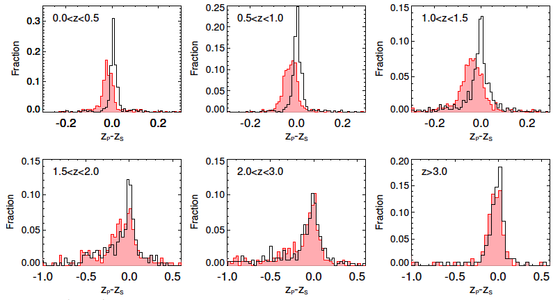
Figure 21.— ($z_{\rm p}-z_{\rm s}$) distribution in various redshift bins. The photo-z are computed using the $\rm{TFIT}_{\rm{CANDELS+IB}}$ photometric catalog and using the templates with (black solid line ) and without (red solid lines) emission line contributions. The upper panel shows that the emission lines are useful particularly at $z<1.5$.

Ilbert et al. (2009) demonstrated the importance of taking emission lines into account for photo-z. Including lines in the templates improved photo-z accuracy by a factor of 2.5 for bright ($i^{+}<22.5$) galaxies in the COSMOS field. The same effect is seen in the deeper $\rm{TFIT}_{\rm{CANDELS+IB}}$ data as shown in Figure 21. Although outlier numbers remain similar ($\sim$4%) whether emission lines are included in the templates or not, the distributions of ($z_{\rm p}-z_{\rm s}$) change. At $z<1.5$, including emission lines gives much narrower peaks and lower bias. At $z>1.5$, the improvement is less than at lower redshifts. Possible reasons are: (a) the contribution of the emission lines are diluted when observed in the NIR bands, which have broader bandwidths than optical bands; (b) the recipes for adding emission lines to the templates may be wrong for high-redshift galaxies; and/or (c) the IB data may be too shallow to affect the high-redshift (and therefore faint) sources. However, even at $z>1.5$, the photo-z accuracy still shows a factor of 1.5 improvement ($\sigma_{\mathrm{NMAD}}$ decreasing from 0.032 to 0.021) when emission lines are included in the templates.

6.4. Testing Libraries for the X-ray Population

Because of the different X-ray populations in the 4Ms-CDFS and 250ks-ECDFS surveys, we adopted different libraries for point-like sources in Areas 1+2 and Area 3. For the sake of template comparison, we tried using the Area 3 (“S09”) library to calculate photo-z for point-like sources in Areas 1+2. The fraction of outliers increased from $5.3\%$ to $15\%$, and the accuracy became two times worse than achieved with the preferred library. Even for $R<23$ sources, $\sigma_{\rm NMAD}$ went from 0.011 with the proper templates to 0.016 with the old ones. For $R>23$ galaxies, the deterioration was from 0.027 to 0.059. In Area 3, on the other hand, using the new templates instead of the S09 ones made photo-z slightly worse: for $R<23$, $\sigma_{\rm NMAD}$ was 0.009 for the new and 0.008 for the S09 libraries. For $R>23$, accuracies were 0.025 and 0.017 respectively. Moreover $\mathrm{bias}_{z}=-0.014$ using the S09 library but increased to $\mathrm{bias}_{z}=-0.031$ with the new library. The better performance of the S09 library in Area 3 can be understood because the population of point-like X-ray sources in the 250k-ECDFS is similar to the XMM-COSMOS population, and the S09 library is more suitable for counterparts of such bright X-ray sources.

6.5. Impact of UV data

UV emission from accretion disks around supermassive black holes makes type 1 AGNs distinguishable from normal galaxies. Therefore including UV data in the photometry is crucial for SED fitting to obtain accurate photo-z and to decrease outliers for AGNs. To demonstrate this we compared photo-z for AGNs obtained with and without photometry in the UV bands. About $25\%$ of all the X-ray detected sources in Areas 1+2+3 have UV data available from GALEX. Among these, 221 sources have spectroscopy available and were used as our test sample. As expected, for the optically extended sources, where the host dominates the emission, there is very little difference in accuracy and fraction of outliers whether UV data are included or not. For 170 extended sources with spectroscopy, including UV data decreases $\sigma_{\mathrm{NMAD}}$ from 0.013 to 0.012 and $\eta$ from $5.9\%$ to $5.3\%$. In contrast, for the 51 point-like (i.e., AGN-dominated) sources, adding the UV data halves the number of outliers (from $23.5\%$ to $11.8\%$) though with only modest improvement in accuracy (from 0.013 to 0.011). Among the five remaining outliers (see Fig. 22), two are faint ($\mathrm{mag}>23$) in the UV, and three are close to other sources with the UV flux blended in the 10″ GALEX aperture. Deblending the GALEX photometry with TFIT as in the other bands could perhaps improve these cases.

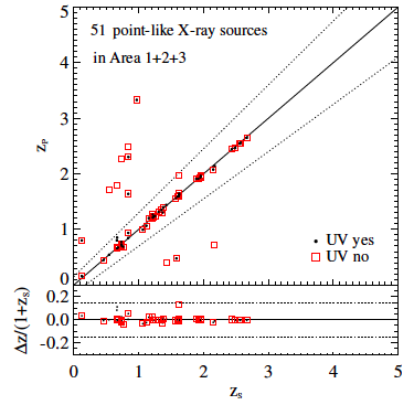
Figure 22.— Comparison of photo-z with spec-z for X-ray sources with point-like counterparts. All 51 available sources in Areas 1+2+3 are plotted. Black dots indicate photo-z computed with UV data, and red squares indicate photo-z computed without UV data.

7. Released Catalogs

Tables 8 through 11 give homogeneously computed photo-z and related data for all sources detected in the area covered by CANDELS/GOODS-S, CDFS, and ECDFS survey. For each source we make also available the redshift probability distribution function $P(z)$. With these data it is possible to construct figures like the inserts in Figure 23. Because of the large size of the $P(z)$ files, we provide them at the link http://www.mpe.mpg.de/XraySurveys. In lieu of the full $P(z)$, the catalogs provide a proxy in the form of the normalized integral of the main probability distribution $P(z_{{p}})\equiv 100\times\int P(z)dz$ with the integral over the range $z_{{p}}\pm 0.1(1+z_{{p}})$. A value close to 100 indicates that the photo-z value is uniquely defined. Smaller values imply that a wide range or multiple photo-z values are possible. Updated versions of the catalogs and templates will be available under [Surveys] $>$ [CDFS] through the portal http://www.mpe.mpg.de/XraySurveys.

For the Chandra X-ray detections, the catalogs also provide a new compilation of X-ray source lists from the literature, the new optical/NIR/MIR associations, and the corresponding photometry. Catalog descriptions and excerpts are below. An entry of -99 indicates no data for that quantity. All coordinates are J2000.

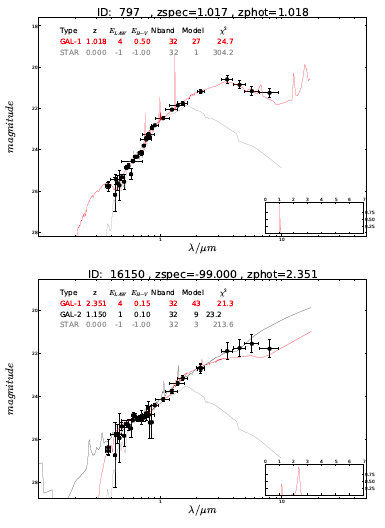
Figure 23.— Two examples of SED fitting for source 797 ( a normal galaxy) and source 16150 (an X-ray-detected AGN). The photometric points are shown in black. The red lines show the best-fitting template, and grey lines the best fitting star (the latter a poor fit for both objects shown). In the right panel, the black line shows the second-best template. Information about the templates—type, photo-z, extinction law, extinction value, number of bands, model identification, and $\chi^{2}$ of the fit—is given in the legends. Inserts show $P(z)$ for the sources.

7.1. Cross ID reference table

Table 8 gives cross-IDs and positions for all sources within each Area as identified in Table 2. The table also indicates whether a source is a possible counterpart to an X-ray detection.

Table 8Column description of the cross ID reference catalog

Column	Title	Description
1	[HSN2014]	Sequential number adopted in this work.
2-4	$\rm{ID_{C}}$ , $\rm{R.A._{C}}$, $\rm{Dec._{C}}$	ID, right ascension and declination from the CANDELS-TFIT catalog (G13).
5-7	$\rm{ID_{M}}$ , $\rm{R.A._{M}}$, $\rm{Dec._{M}}$	ID, right ascension and declination from the MUSYC catalog (Cardamone et al., 2010).
8-10	$\rm{ID_{T}}$, $\rm{R.A._{T}}$, $\rm{Dec._{T}}$	ID, right ascension and declination from the TENIS catalog (Hsieh et al., 2012).
11-13	$\rm{ID_{S}}$, $\rm{R.A._{S}}$, $\rm{Dec._{S}}$	ID, right ascension and declination from the SIMPLE catalog (Damen et al., 2011).
14-17	$\rm{ID_{R13}}$, $\rm{R.A._{R13}}$, $\rm{Dec._{R13}}$, $\rm{PosErr_{R13}}$	ID, right ascension, declination and positional error from the R13 4Ms-CDFS catalog.
18-21	$\rm{ID_{X11}}$, $\rm{R.A._{X11}}$, $\rm{Dec._{X11}}$, $\rm{PosErr_{X11}}$	ID, right ascension, declination and positional error from the X11 4Ms-CDFS catalog.
22-25	$\rm{ID_{L05}}$, $\rm{R.A._{L05}}$, $\rm{Dec._{L05}}$, $\rm{PosErr_{L05}}$	ID, right ascension, declination and positional error from the L05 250ks-ECDFS catalog.
26-29	$\rm{ID_{V06}}$, $\rm{R.A._{V06}}$, $\rm{Dec._{V06}}$, $\rm{PosErr_{V06}}$	ID, right ascension, declination and positional error from the V06 250ks-ECDFS catalog.
30	Xflag	“1” indicates that the source is the only possible counterpart to an X-ray source.
		“n” (2 or more) indicates that the source is one of the “n” possible counterparts
		for a give X-ray source. “-99” indicates that no X-ray counterpart are found.
31	$p$	Posterior value which indicates the reliability of the X-ray to optical/NIR/MIR association.
		(as defined in Section 3.2)

7.2. X-ray source list in ECDFS

Table 9X-ray source list

[HSN2014]	$\rm{ID_{R13}}$	$\rm{ID_{X11}}$	$\rm{ID_{L05}}$	$\rm{ID_{V06}}$	$\rm{R.A._{x}}$	$\rm{DEC._{x}}$	$\rm{Flux_{s}}$	$\rm{Flux_{h}}$	$\rm{Flux_{f}}$	log $L_{\rm{s}}$	log $L_{\rm{h}}$	log $L_{\rm{f}}$
(1)	(2)	(3)	(4)	(5)	(6)	(7)	(8)	(9)	(10)	(11)	(12)	(13)
125	343	266	-99	-99	53.079439	-27.949429	2.05E-16	7.62E-16	9.86E-16	41.28	41.85	41.969
482	6	336	-99	-99	53.103424	-27.933357	8.84E-16	3.67E-15	4.59E-15	42.37	42.99	43.085
47821	-99	-99	527	445	53.251375	-27.980556	1.06E-15	2.33E-15	3.22E-15	42.66	43.00	43.14
50721	-99	-99	32	348	52.842417	-27.965417	2.07E-15	1.61E-14	1.81E-14	42.14	43.03	43.08

Table 9 gives the X-ray source list in Areas 1+2+3 with the position and flux information from the available catalogs. Columns are as follows:
(1) [HSN2014]: Sequential number adopted in this work.
(2) $\rm{ID_{R13}}$: ID from R13 catalog
(3) $\rm{ID_{X11}}$: ID from X11 catalog
(4) $\rm{ID_{L05}}$: ID from L05 catalog
(5) $\rm{ID_{V06}}$: ID from V06 catalog
(6) $\rm{R.A._{x}}$: Right Ascension of the X-ray source.
(7) $\rm{DEC._{x}}$: Declination of the X-ray sources.
(8) $\rm{Flux_{s}}$: Soft band X-ray flux ($\rm{erg~{}cm^{-2}~{}s^{-1}}$).
(9) $\rm{Flux_{h}}$: Hard band X-ray flux.
(10) $\rm{Flux_{f}}$: Full band X-rayflux.
(11) log $L_{\rm{s}}$: Soft band X-ray luminosity ($\rm{erg~{}s^{-1}}$).
(12) log $L_{\rm{h}}$: Hard band X-ray luminosity.
(13) log $L_{\rm{f}}$: Full band X-ray luminosity.
Note: From column (6) to (10), we chose the original X-ray data from, in order of priority, R13, X11, L05 and V06.

7.3. Photometry of X-ray sources

Table 10 gives photometry for all the possible counterparts to the X-ray sources. For the CANDELS area, this includes the TFIT photometry in the IBs as described in Section 2.1. Columns are as follows:
(1) [HSN2014]: Sequential number adopted in this work.
(2)-(5) XID: ID from the four X-ray catalogs with the same order as Table 9
(6)Xflag: As described in Table 8
(7)$p$: As described in Table 8
(8)$\rm{R.A._{opt}}$: Right Ascension of the optical/NIR/MIR source.
(9)$\rm{Dec._{opt}}$: Declination of the optical/NIR/MIR source.
(10)-(109): AB magnitude and the associated uncertainty in each of possible bands (Table 1).

Table 10Photometry of X-ray sources

[HSN2014]	XID	xflag	p	$\rm{R.A._{opt}}$	$\rm{Dec._{opt}}$	$\rm{FUV_{m}}$	$\rm{FUV_{e}}$	$\rm{NUV_{m}}$	$\rm{NUV_{e}}$	…	…	$\rm{IRAC4_{m}}$	$\rm{IRAC4_{e}}$
(1)	(2)-(5)	(6)	(7)	(8)	(9)	(10)	(11)	(12)	(13)	…	…	(108)	(109)
125	…	2	0.98	53.079489	-27.948735	-99.0	-99.0	-99.0	-99.0	…	…	19.888	0.016
482	…	1	0.99	53.103520	-27.933323	-99.0	-99.0	-99.0	-99.0	…	…	21.096	0.03
47821	…	2	0.97	53.252067	-27.980645	-99.0	-99.0	-99.0	-99.0	…	…	22.421	0.18
50721	…	2	1.0	52.84249	-27.965261	-99.0	-99.0	-99.0	-99.0	…	…	19.24	0.032

7.4. Redshift catalog

Table 11Redshift catalog

[HSN2014]	$\rm{R.A._{opt}}$	$\rm{Dec._{opt}}$	$z_{s}$	$Q_{\rm{zs}}$	$z_{p}$	$1\sigma^{\rm{low}}$	$1\sigma^{\rm{up}}$	$3\sigma^{\rm{low}}$	$3\sigma^{\rm{up}}$	$P(z_{\rm{p}}$)	$z_{\rm{p}}2$	$P(z_{\rm{p}}2$)	$N_{\rm{p}}$	Mod	xflag	$p$
(1)	(2)	(3)	(4)	(5)	(6)	(7)	(8)	(9)	(10)	(11)	(12)	(13)	(14)	(15)	(16)	(17)
13	53.093452	-27.957135	-99.0	-99	3.2619	3.25	3.27	3.21	3.29	100.0	-99.0	0.0	29	328	-99	-99
14	53.104490	-27.957068	-99.0	-99	2.1768	0.44	2.23	0.43	2.46	91.05	0.45	8.91	27	331	-99	-99
15	53.088446	-27.956996	-99.0	-99	3.0468	3.01	3.09	2.92	3.18	100.0	-99.0	0.0	26	322	-99	-99
16	53.104181	-27.956592	-99.0	-99	3.1233	3.05	3.19	2.93	3.28	99.99	-99.0	0.0	27	324	-99	-99
125	53.079490	-27.94874	0.619	0	0.6664	0.66	0.68	0.65	0.68	100.0	-99.0	0.0	24	028	2	0.98
135	53.142288	-27.94447	-99.0	-99	2.6422	2.5	2.72	1.11	3.07	66.19	1.17	13.80	27	014	1	0.95

Table 11 gives photo-z results for all sources detected in the CANDELS/GOODS-S, CDFS and ECDFS area. X-ray detections are flagged in the catalog. Columns are:
(1) [HSN2014]: Sequential number adopted in this work.
(2) $\rm{R.A._{opt}}$: Right Ascension of the optical/NIR/MIR source.
(3) $\rm{Dec._{opt}}$: Declination of the optical/NIR/MIR source.
(4) $z_{\rm{s}}$: Spectroscopic redshift (N. Hathi, private communication).
(5) $Q_{\rm{zs}}$: Quality of the spectroscopic redshift. (0=High, 1=Good, 2=Intermediate, 3=Poor).
(6) $z_{\rm{p}}$: The photo-z value as defined by the minimum of $\chi^{2}$.
(7) $1\sigma^{\rm{low}}$: Upper $1\sigma$ value of the photo-z.
(8) $1\sigma^{\rm{up}}$: Lower $1\sigma$ value of the photo-z.
(9) $3\sigma^{\rm{low}}$: Upper $2.3\sigma$ value of the photo-z.
(10) $3\sigma^{\rm{up}}$: Lower $2.3\sigma$ value of the photo-z.
(11) $P(z_{{p}})$: Normalized area under the curve $P(z)$, computed between $z_{\rm{p}}\pm 0.1(1+z_{{p}})$.
(12) $z_{{p}}2$: The second solution in the photo-z, when the $P(z_{{p}2})$ is above 5.
(13) $P(z_{{p}2})$: Normalized area under the curve $P(z)$, computed between $z_{{p2}}\pm 0.1(1+z_{{p2}})$.
(14) $N_{\rm{p}}$: Number of photometric points used in the fit.
(15) Mod: Template number used for SED fitting. 1-48 are the templates from Lib-EXT; 101-130 are the templates from Lib-PT; 201-230 are the templates from S09; 301-331 are the templates from Ilbert et al. (2009), in the same order as the mentioned authors used.
(16) Xflag: As described in Table 8
(17) $p$: Posterior value which indicates the reliability of the X-ray to Optical/NIR/MIR association (as defined in Section 3.2).

8. Summary

The main product of this work is photometric redshifts for all sources detected in the CANDELS/GOODS-S, CDFS, and ECDFS area, a total of 105150 sources. This work has improved upon prior catalogs by G13, Cardamone et al. (2010) and Hsieh et al. (2012) by using the most up-to-date photometry and SED template libraries including separate libraries for X-ray sources of different characteristics. Probabilities of association between X-ray sources and optical/NIR/MIR sources are also provided.

Our work has improved photo-z in the fields in the following ways:

1. In the CANDELS area, we added the IB photometry from Subaru (Cardamone et al., 2010) to the space-based photometric catalog of Guo et al. (2013) using the same TFIT parameters as in the official CANDELS catalog. The combined effect of using IB photometry to pinpoint emission lines in the objects and including lines in the templates gives excellent results, even for faint and high redshift sources (Table 4 and Table 6).

2. Using homogeneous data from the CANDELS/$H$-band, TENIS/$J\&K$ , MUSYC/$BVR$, and IRAC-3.6$\mu\mathrm{m}$-selected catalogs, we made X-ray to multi-wavelength associations simultaneously by means of a new, fast matching algorithm based on Bayesian statistics. This gave $98\%$, $96\%$, and $94\%$ of X-ray sources with reliable counterparts in Areas 1,  2, and 3, respectively. Despite the new technique and data, all but 7 associations are consistent with those found earlier by by X11. The 7 new associations come from the deep, high-resolution CANDELS images and TENIS images that were not available earlier. Different X-ray reduction procedures can change the X-ray position by a few arcseconds. In crowded areas this may imply a different X-ray to optical association.

3. We demonstrated that the X-ray properties of sources need to be taken into account when constructing the library of templates for computing photo-z for such sources. More specifically, the library defined by Salvato et al. (2009, 2011) for the rare X-ray bright sources detected in COSMOS is not representative of the faint X-ray source population detected in the deeper 4Ms-CDFS. We therefore defined a new of galaxy/AGN hybrids for the 4Ms survey (Areas 1+2). In the 250ks survey (Area 3), where the X-ray data have a depth similar to Chandra-COSMOS, the Salvato et al. (2009) template library with the Salvato et al. (2011) selection strategy works well.

Appendix A AGN-Galaxy Hybrid Templates

We built hybrid templates by combining one of two AGN templates with a set of normal galaxy templates in various proportions. The Type 1 AGN template was derived from “TQSO1” of Polletta et al. (2007). Salvato et al. (2009) added a UV power-law to give “pl-TQSO1.” The Type 2 AGN template was “QSO2” unchanged from Polletta et al. (2007).

The galaxy templates were 32 semi-empirical ones from Bender et al. (2001) (see Fig. 24). These templates were constructed by first sorting galaxies of known spec-z in the FORS Deep Field (Appenzeller et al., 2004; Gabasch et al., 2004) iteratively into 32 bins of similar spectral shape. Broad-band fluxes from the $U$-band to the $K$-band of typically ten galaxies at different redshifts were combined to obtain one broadband template covering as wide a wavelength range as possible. These broad-band empirical templates were fitted by a combination of model spectral energy distributions from Bruzual & Charlot (2003) and Maraston (2005) and empirical spectra from Noll et al. (2004) to obtain “semi-empirical” templates with spectral resolution $R\sim 1000$. The method covered wavelengths from $\sim$60 nm to 2.5 $\mu$m. Figure 25 illustrates two of the templates in use.

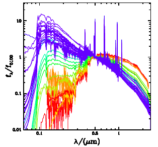
Figure 24.— Galaxy templates from Bender et al. (2001), color coded as a function of activity from the redder passive galaxies to the bluer strongly star forming objects.

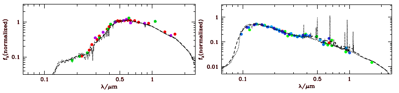
Figure 25.— Galaxy templates in use for photometric redshift estimation. Colored symbols represent broad-band flux densities of individual galaxies with known spec-z. The short-dashed line shows the $R\sim 1000$ spectral template best fitting the broadband flux densities after smoothing to the broad-band resolution. The smoothed template is shown as a long-dashed line.

Making the hybrid templates followed the procedure of Salvato et al. (2009). First we normalized both AGN and galaxy templates at 5500 Å, then combined them with the AGN-to-galaxy ratio changing from 1:9 to 9:1. (See examples in Fig. 26.) In total, 576 hybrids were created this way. We then randomly chose $25\%$ of spectroscopic X-ray sources (52 extended sources and 62 point-like sources) to train the hybrids. As Figure 2 has shown, the training samples are well distributed over the entire ranges of redshift and magnitude. We treated the extended and point-like sources separately, fixing the redshift at the spectroscopically defined value and choosing the templates most frequently selected to represent the training sources. After several iterations, we obtained the libraries used for the extended sources (Lib-EXT: 31 hybrids + 17 galaxy templates, see Fig. 27) and for the point-like sources (Lib-PT: 30 hybrids, see Fig. 28).

Table 12 lists the templates in Lib-EXT and Lib-PT. Names with ”-TQSO1-” or ”-QSO2-” indicate the AGN component used. The number following indicates the fractional AGN contribution in the hybrid. For example, the template “s050-8-TQSO1-2” contains $80\%$ galaxy (s050) and $20\%$ of AGN (TQOS1) . The templates without TQSO1 and QSO2 are pure galaxies with different levels of star formation. (See Bender et al. 2001 for details.)

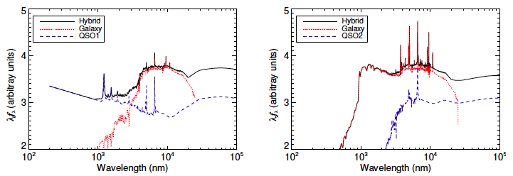
Figure 26.— Two examples of hybrid SED templates. Red lines show the galaxy contribution, blue lines the AGN contribution, and black lines the sum. The left panel shows is a hybrid comprised of 10% Type 1 AGN and 90% galaxy. The right panel shows a hybrid with 30% Type 2 QSO and 70% starburst galaxy.

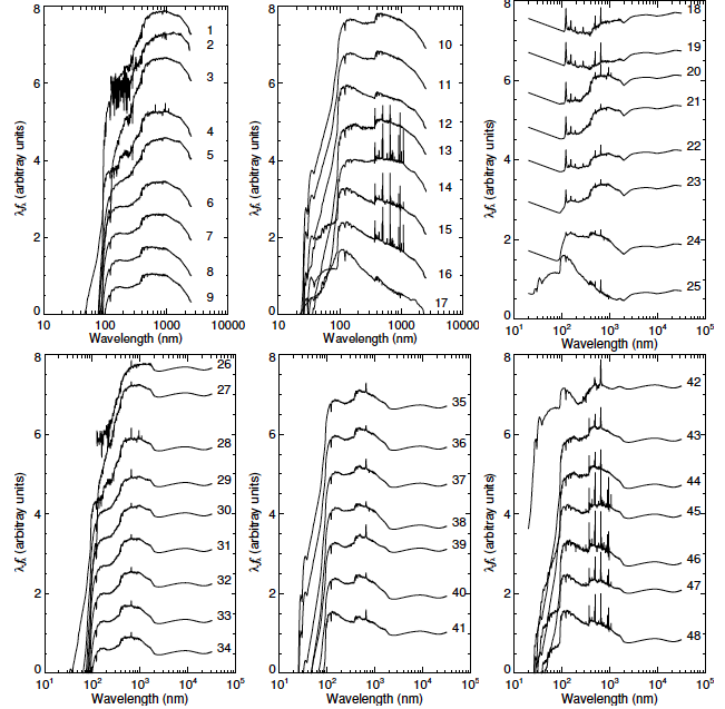
Figure 27.— SEDs for all templates in Lib-EXT.

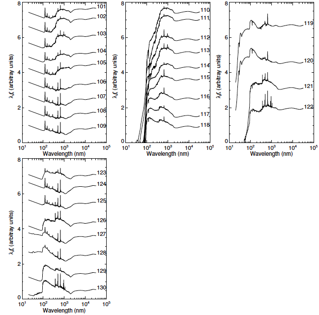
Figure 28.— SEDs for all templaes in Lib-PT.

Table 12The list of AGN-galaxy hybrids in Lib-EXT and Lib-PT.

Lib-EXT		Lib-PT
No.	Template	No.	Template
1	mod-e	101	e-8-TQSO1-2
2	manucci-sbc	102	s010-9-TQSO1-1
3	mod-s010	103	s020-9-TQSO1-1
4	mod-s020	104	s050-8-TQSO1-2
5	mod-s030	105	sac-7-TQSO1-3
6	mod-s070	106	ec-3-TQSO1-7
7	mod-s090	107	sac-2-TQSO1-8
8	mod-s120	108	s010-3-TQSO1-7
9	mod-s150	109	s180-3-TQSO1-7
10	mod-s200	110	e-9-QSO2-1
11	mod-s400	111	s010-9-QSO2-1
12	mod-s500	112	s020-7-QSO2-3
13	mod-fdf4	113	s020-9-QSO2-1
14	mod-s210	114	s050-9-QSO2-1
15	mod-s670	115	s090-6-QSO2-4
16	mod-s700	116	s200-7-QSO2-3
17	mod-s800	117	s400-9-QSO2-1
18	ec-6-TQSO1-4	118	s500-8-QSO2-2
19	sac-5-TQSO1-5	119	s800-2-QSO2-8
20	s020-9-TQSO1-1	120	s800-5-QSO2-5
21	s030-9-TQSO1-1	121	fdf4-9-QSO2-1
22	s050-8-TQSO1-2	122	s230-5-QSO2-5
23	s070-9-TQSO1-1	123	s250-8-TQSO1-2
24	s250-9-TQSO1-1	124	s250-1-TQSO1-9
25	s800-8-TQSO1-2	125	fdf4-4-TQSO1-6
26	sac-9-QSO2-1	126	fdf4-9-TQSO1-1
27	s010-9-QSO2-1	127	s800-2-TQSO1-8
28	s020-9-QSO2-1	128	s800-4-TQSO1-6
29	s050-8-QSO2-2	129	s500-9-TQSO1-1
30	s050-9-QSO2-1	130	s670-9-TQSO1-1
31	s070-9-QSO2-1
32	s090-9-QSO2-1
33	s120-9-QSO2-1
34	s180-9-QSO2-1
35	s200-8-QSO2-2
36	s200-9-QSO2-1
37	s250-8-QSO2-2
38	s250-9-QSO2-1
39	s400-7-QSO2-3
40	s400-9-QSO2-1
41	s500-8-QSO2-2
42	s800-1-QSO2-9
43	fdf4-7-QSO2-3
44	fdf4-9-QSO2-1
45	s230-8-QSO2-2
46	s650-9-QSO2-1
47	s670-6-QSO2-4
48	s670-9-QSO2-1

References

- Aird et al. (2010) Aird, J., Nandra, K., Laird, E. S., et al. 2010, MNRAS, 401, 2531
- Appenzeller et al. (2004) Appenzeller, I., Bender, R., Böhm, A., et al. 2004, The Messenger, 116, 18
- Arnouts et al. (1999) Arnouts, S., Cristiani, S., Moscardini, L., et al. 1999, MNRAS, 310, 540
- Ashby et al. (2013) Ashby, M. L. N., Willner, S. P., Fazio, G. G., et al. 2013, ApJ, 769, 80
- Bender et al. (2001) Bender, R., Appenzeller, I., Böhm, A., et al. 2001, in Deep Fields, ed. S. Cristiani, A. Renzini, & R. E. Williams, 96
- Benítez et al. (2009) Benítez, N., Moles, M., Aguerri, J. A. L., et al. 2009, ApJ, 692, L5
- Brusa et al. (2007) Brusa, M., Zamorani, G., Comastri, A., et al. 2007, ApJS, 172, 353
- Bruzual & Charlot (2003) Bruzual, G., & Charlot, S. 2003, MNRAS, 344, 1000
- Budavári & Szalay (2008) Budavári, T., & Szalay, A. S. 2008, ApJ, 679, 301
- Calzetti et al. (2000) Calzetti, D., Armus, L., Bohlin, R. C., et al. 2000, ApJ, 533, 682
- Cappelluti et al. (2009) Cappelluti, N., Brusa, M., Hasinger, G., et al. 2009, A&A, 497, 635
- Cardamone et al. (2008) Cardamone, C. N., Urry, C. M., Damen, M., et al. 2008, ApJ, 680, 130
- Cardamone et al. (2010) Cardamone, C. N., van Dokkum, P. G., Urry, C. M., et al. 2010, ApJS, 189, 270
- Castellano et al. (2007) Castellano, M., Salimbeni, S., Trevese, D., et al. 2007, ApJ, 671, 1497
- Civano et al. (2012) Civano, F., Elvis, M., Brusa, M., et al. 2012, ApJS, 201, 30
- Daddi et al. (2004) Daddi, E., Cimatti, A., Renzini, A., et al. 2004, ApJ, 617, 746
- Dahlen et al. (2013) Dahlen, T., Mobasher, B., Faber, S. M., et al. 2013, ApJ, 775, 93
- Damen et al. (2011) Damen, M., Labbé, I., van Dokkum, P. G., et al. 2011, ApJ, 727, 1
- Dehghan & Johnston-Hollitt (2014) Dehghan, S., & Johnston-Hollitt, M. 2014, AJ, 147, 52
- Donley et al. (2012) Donley, J. L., Koekemoer, A. M., Brusa, M., et al. 2012, ApJ, 748, 142
- Drory et al. (2005) Drory, N., Salvato, M., Gabasch, A., et al. 2005, ApJ, 619, L131
- Elvis et al. (2009) Elvis, M., Civano, F., Vignali, C., et al. 2009, ApJS, 184, 158
- Feulner et al. (2005) Feulner, G., Gabasch, A., Salvato, M., et al. 2005, ApJ, 633, L9
- Fotopoulou et al. (2012) Fotopoulou, S., Salvato, M., Hasinger, G., et al. 2012, ApJS, 198, 1
- Gabasch et al. (2004) Gabasch, A., Bender, R., Seitz, S., et al. 2004, A&A, 421, 41
- Gabasch et al. (2006) Gabasch, A., Hopp, U., Feulner, G., et al. 2006, A&A, 448, 101
- Giavalisco et al. (2004) Giavalisco, M., Ferguson, H. C., Koekemoer, A. M., et al. 2004, ApJ, 600, L93
- Grazian et al. (2006) Grazian, A., Fontana, A., de Santis, C., et al. 2006, A&A, 449, 951
- Grogin et al. (2011) Grogin, N. A., Kocevski, D. D., Faber, S. M., et al. 2011, ApJS, 197, 35
- Guo et al. (2013) Guo, Y., Ferguson, H. C., Giavalisco, M., et al. 2013, ApJS, 207, 24
- Hsieh et al. (2012) Hsieh, B.-C., Wang, W.-H., Hsieh, C.-C., et al. 2012, ApJS, 203, 23
- Ilbert et al. (2006) Ilbert, O., Arnouts, S., McCracken, H. J., et al. 2006, A&A, 457, 841
- Ilbert et al. (2009) Ilbert, O., Capak, P., Salvato, M., et al. 2009, ApJ, 690, 1236
- Koekemoer et al. (2011) Koekemoer, A. M., Faber, S. M., Ferguson, H. C., et al. 2011, ApJS, 197, 36
- Laidler et al. (2007) Laidler, V. G., Papovich, C., Grogin, N. A., et al. 2007, PASP, 119, 1325
- Laird et al. (2009) Laird, E. S., Nandra, K., Georgakakis, A., et al. 2009, ApJS, 180, 102
- Lehmer et al. (2005) Lehmer, B. D., Brandt, W. N., Alexander, D. M., et al. 2005, ApJS, 161, 21
- Luo et al. (2010) Luo, B., Brandt, W. N., Xue, Y. Q., et al. 2010, ApJS, 187, 560
- Maraston (2005) Maraston, C. 2005, MNRAS, 362, 799
- Matute et al. (2012) Matute, I., Márquez, I., Masegosa, J., et al. 2012, A&A, 542, A20
- Merloni et al. (2012) Merloni, A., Predehl, P., Becker, W., et al. 2012, ArXiv e-prints, arXiv:1209.3114
- Naylor et al. (2013) Naylor, T., Broos, P. S., & Feigelson, E. D. 2013, ApJS, 209, 30
- Noll et al. (2004) Noll, S., Mehlert, D., Appenzeller, I., et al. 2004, A&A, 418, 885
- Polletta et al. (2007) Polletta, M., Tajer, M., Maraschi, L., et al. 2007, ApJ, 663, 81
- Prevot et al. (1984) Prevot, M. L., Lequeux, J., Prevot, L., Maurice, E., & Rocca-Volmerange, B. 1984, A&A, 132, 389
- Quadri & Williams (2010) Quadri, R. F., & Williams, R. J. 2010, ApJ, 725, 794
- Rangel et al. (2013) Rangel, C., Nandra, K., Laird, E. S., & Orange, P. 2013, MNRAS, 428, 3089
- Rosario et al. (2013) Rosario, D. J., Mozena, M., Wuyts, S., et al. 2013, ApJ, 763, 59
- Salimbeni et al. (2009) Salimbeni, S., Castellano, M., Pentericci, L., et al. 2009, A&A, 501, 865
- Salvato et al. (2009) Salvato, M., Hasinger, G., Ilbert, O., et al. 2009, ApJ, 690, 1250
- Salvato et al. (2011) Salvato, M., Ilbert, O., Hasinger, G., et al. 2011, ApJ, 742, 61
- Scoville et al. (2007) Scoville, N., Abraham, R. G., Aussel, H., et al. 2007, ApJS, 172, 38
- Spergel et al. (2003) Spergel, D. N., Verde, L., Peiris, H. V., et al. 2003, ApJS, 148, 175
- Sutherland & Saunders (1992) Sutherland, W., & Saunders, W. 1992, MNRAS, 259, 413
- Taylor (2005) Taylor, M. B. 2005, in Astronomical Society of the Pacific Conference Series, Vol. 347, Astronomical Data Analysis Software and Systems XIV, ed. P. Shopbell, M. Britton, & R. Ebert, 29
- Virani et al. (2006) Virani, S. N., Treister, E., Urry, C. M., & Gawiser, E. 2006, AJ, 131, 2373
- Wuyts et al. (2008) Wuyts, S., Labbé, I., Schreiber, N. M. F., et al. 2008, ApJ, 682, 985
- Xue et al. (2011) Xue, Y. Q., Luo, B., Brandt, W. N., et al. 2011, ApJS, 195, 10
- Zheng et al. (2004) Zheng, W., Mikles, V. J., Mainieri, V., et al. 2004, ApJS, 155, 73