Initial data for high-compactness black hole–neutron star binaries

Abstract

For highly compact neutron stars, constructing numerical initial data for black hole–neutron star binary evolutions is very difficult. We describe improvements to an earlier method that enable it to handle these more challenging cases. We examine the case of a 6:1 mass ratio system in inspiral close to merger, where the star is governed by a polytropic $\Gamma=2$, an SLy, or an LS220 equation of state. In particular, we are able to obtain a solution with a realistic LS220 equation of state for a star with compactness $0.26$ and mass $1.98\text{\,}\text{$M_{\odot}$}$, which is representative of the highest reliably determined neutron star masses. For the SLy equation of state, we can obtain solutions with a comparable compactness of 0.25, while for a family of polytropic equations of state, we obtain solutions with compactness up to $0.21$, the largest compactness that is stable in this family. These compactness values are significantly higher than any previously published results. We find that improvements in adapting the computational domain to the neutron star surface and in accounting for the center of mass drift of the system are the key ingredients allowing us to obtain these solutions.

I Introduction

Among the prime candidate sources for ground-based gravitational wave detectors are binary systems containing inspiraling neutron stars: black hole–neutron star (BHNS) binaries, or systems containing two neutron stars. Besides being likely gravitational wave sources, such systems are the leading candidates to explain short gamma-ray bursts Eichler et al. (1989); Narayan et al. (1992); Mochkovitch et al. (1993); Lee and Kluźniak (1998); Janka et al. (1999). Radioactive decay of the neutron-rich material ejected by the merger may also power optical/infrared transients days after the merger Roberts et al. (2011); Metzger and Berger (2012); Tanaka et al. (2014), particularly for BHNS binaries with a large neutron star and a rapidly rotating black hole Foucart et al. (2013); Kyutoku et al. (2013); Lovelace et al. (2013); Deaton et al. (2013); Foucart et al. (2014), and for binary neutron star mergers with compact neutron stars Hotokezaka et al. (2013).

Gravitational waves from coalescing binaries are searched for and analyzed using the matched-filtering technique Finn (1992); Finn and Chernoff (1993); Abadie et al. (2011); Babak et al. (2012), which compares the detector output with a bank of templates that model the waves emitted by the source. Therefore accurate knowledge of the expected waveforms of incoming signals is required. While post-Newtonian templates are expected to be accurate when the binary is widely separated, they break down near merger. Fully relativistic numerical simulations of the last few orbits and the merger are needed to match onto the post-Newtonian waveforms. Moreover, modeling of the subsequent electromagnetic and neutrino emission must also be done by a code that can deal with all the effects of strong-field gravity.

Numerical modeling of these systems is very challenging (see Duez (2010); Shibata and Taniguchi (2011); Faber and Rasio (2012); Lehner and Pretorius (2014) for reviews). A key ingredient in such simulations is accurate initial data. Ideally, one would like a snapshot of the gravitational field and the matter distribution only a few orbits before merger but resulting from millions of years of slow inspiral. In general relativity, no exact way is known to do this because the nonlinear Einstein equations are too difficult to solve. So instead, various plausible approximations are made. The most common assumption is that the binary has had time to settle into a quasi-equilibrium state, the system being approximately time-independent in the corotating frame. Furthermore, as the viscous forces within the star are expected to be small, we do not expect much change in the spin of the star as the orbital radius decreases. For an initially nonspinning neutron star, this would lead to an irrotational velocity profile, another standard assumption. Because of gravitational wave emission, however, there is no exact equilibrium state. Accordingly, these conditions cannot all be perfectly satisfied simultaneously. Nevertheless, initial data incorporating these assumptions seems to work quite well in practice.

This paper will focus on initial data for BHNS binaries, and in particular systems where the neutron star has high compactness

$$\mathcal{C}=\frac{M_{\mathrm{NS}}}{R}.$$ (1)

Here $M_{\mathrm{NS}}$ is the ADM mass and $R$ is the areal radius for an isolated star with the same equation of state and baryon mass, and we use units with $c=G=1$. The techniques introduced here should be equally applicable to neutron star–neutron star binaries.

Previous results on initial data for BHNS evolutions include the early work of Taniguchi et al. Taniguchi et al. (2005) and Sopuerta et al. Sopuerta et al. (2006), as well as more recent initial configurations generated by Taniguchi et al. Taniguchi et al. (2006, 2007, 2008) and Grandclement Grandclément (2006). Both Taniguchi and Grandclement use codes based on the LORENE package Gourgoulhon et al. (2012), and excise from the computational domain the region inside the apparent horizon of the black hole. An alternative method based on the puncture formalism, in which the constraints are solved both inside and outside the black hole horizon, has been proposed by Kyutoku et al. Kyutoku et al. (2009). The results from Kyutoku et al. (2009) were also obtained using LORENE. A newer initial data code, COCAL, has been developed by Uryū and Tsokaros Uryū and Tsokaros (2012), but not yet applied to BHNS binaries.

Our own group has developed an independent code (Foucart et al. (2008), henceforth Paper I) that uses a multidomain spectral method to achieve high accuracy at a relatively low computational cost. The code is based on the spectral elliptic solver (Spells) developed by the Cornell-Caltech collaboration  Pfeiffer and York (2003), and originally developed by Pfeiffer Pfeiffer et al. (2002, 2003) for the study of binary black hole initial data. While the mathematical formulation of the problem is very similar to Taniguchi et al. (2008) and Grandclément (2006), the numerical techniques are quite different. In particular, while all use multidomain spectral methods, the flexibility that Spells offers in choosing subdomain shapes and the form of the elliptic equations allows one to efficiently adapt the configuration of the numerical grid to the geometry of the system and obtain high-precision results at a very reasonable computational cost.

A drawback of the method described in Paper I is that it fails to converge to a solution when the compactness $\mathcal{C}$ of the neutron star is too high. In fact, this seems to be a defect of all the published methods for solving the BHNS initial value problem. The maximum compactness that can be handled depends on the equation of state (EOS). The easiest EOS for all methods is a $\Gamma=2$ polytrope because it is smooth inside the star, and the density goes linearly to zero near the surface. The method of Paper I can reliably produce binaries with an initial separation of $7M_{0}$ and a compactness up to 0.18. Here $M_{0}$ is defined via

$$M_{0}=M_{\mathrm{BH}}+M_{\mathrm{NS}}$$ (2)

where $M_{\rm BH}$ is the Christodoulou mass of the black hole and $M_{\rm NS}$ is the neutron star mass as defined above. With some small modifications, described later, it can reach $\mathcal{C}=0.20$, very close to the maximum allowed value before the neutron star is unstable to gravitational collapse.

Treating realistic equations of state is more difficult. They tend to have nonsmooth behavior as the composition changes in various density regimes. They often have nonanalytic behavior or very steep slopes at the surface. And even smooth equations of state may be given in tabular form, which introduces its own nonsmoothness. For example, for the SLy EOS Douchin and Haensel (2001); Haensel and Potekhin (2004); Shibata et al. (2005), the maximum compactness attainable by the method of Paper I is 0.16, corresponding to a neutron star mass of $1.27\text{\,}\text{$M_{\odot}$}$. The other codes for producing BHNS initial data have reported a maximum compactness of $\mathcal{C}=0.196$ with a piecewise-polytropic equation of state (for a $1.45M_{\odot}$ neutron star) Kyutoku et al. (2011), while binary neutron star initial data has been obtained up to $\mathcal{C}=0.213$ (for a $1.6M_{\odot}$ neutron star) Hotokezaka et al. (2013). Since a neutron star of mass $2\text{\,}\text{$M_{\odot}$}$ is known to exist, this is clearly not adequate.

In this paper, we describe several technical improvements to the algorithm of Paper I that allow high-compactness initial data to be calculated. For example, we show that for the SLy EOS, a solution with $\mathcal{C}=0.25$, corresponding a neutron star mass of $1.86\text{\,}\text{$M_{\odot}$}$, can be obtained. Furthermore, for the LS220 EOS Lattimer and Swesty (1991), we can obtain a solution with $\mathcal{C}=0.26$, corresponding to a mass of $1.98\text{\,}\text{$M_{\odot}$}$. These initial data can now be used in binary evolutions to study the effect of high compactness on the outcome of the merger.

In Cordero-Carrión et al. (2009), it was observed that highly compact configurations may result in mathematical nonuniqueness of the solution, and a resolution of this problem was presented in the context of conformally flat formulations for the evolution equations. In contrast, the work reported here is not related to nonuniqueness. Rather, we are dealing with an iterative algorithm that displays poor convergence as the compactness increases. The improvements to the algorithm restore good convergence.

In this paper, we first describe in Section II the methods we use to improve the solution procedure of Paper I, in particular addressing requirements on the proper determination of the neutron star surface location and the control of linear momentum in the system. In Section III we present high compactness results using polytropic, SLy, and LS220 EOS. Finally, in Section IV we offer closing remarks on these findings.

II Methods

Our work is based on an implementation in the Spectral Einstein Code (SpEC) of the procedure described in Paper I. The core of the solution procedure is to solve a set of elliptic equations to determine the metric and the velocity potential for the matter (an “elliptic solve”). These elliptic equations contain a number of auxiliary variables that determine the physical properties of the initial data. Some of these are imposed based on analytical considerations, such as the background metric or boundary conditions, while others are solved for in between iterations in order to enforce desired physical properties (mass and spin of the compact objects, orbital parameters of the binary, total linear momentum of the system), or computationally convenient properties (alignment of the surface of the neutron star with the boundary between two subdomains). This procedure is described in detail in Sec. III.C of Paper I.

In solving the elliptic equations, a relaxation scheme is used to keep the solution in a convergent regime. Instead of simply using the new solution at every step, it is combined with the previous one via

$$u_{\mathrm{new}}=\lambda u^{*}+(1-\lambda)u_{\mathrm{old}}$$ (3)

where $\lambda$ is a parameter (the relaxation parameter) that we can choose, $u$ is a quantity such as the value of the metric at some point, and $u^{*}$ is the value of $u$ found by solving the elliptic equations. This scheme decreases the change in the quantities at each step, which helps to maintain the convergence of the solver. In Paper I, we used $\lambda=0.3$.

In this paper, we show that in order to obtain initial data for high-compactness neutron stars, modifications to the iterative procedure of Paper I are required. In particular, we need to modify how we enforce that the location of the surface of the neutron star is at a subdomain boundary and that the total linear ADM momentum of the system is zero.

II.1 Neutron Star Surface Adjustment

An important aspect of the solver is the numerical domain that is used to solve the equations. We employ the domain described in Paper I Section III.A, and shown here in Fig. 1. The physical domain is covered by a number of overlapping spectral subdomains; choosing the location and resolution of the subdomains allows the domain to be well-matched to the problem. A particularly important detail (we have found) is that since the neutron star surface is a physical discontinuity, it should be placed at a subdomain boundary to avoid Gibbs oscillations in the numerical solution. This requirement was also found in Paper I, although we used a different technique to enforce it. We employ a modification of the method described in Paper I in Section III.A.2 and in item 3 of the iterative procedure of Section III.C.

Figure 1: The domain used for the binary black hole–neutron star system. The horizon of the black hole is an external boundary of the domain; its interior is excised. The thick line shows the star surface; this and all other interior lines form subdomain boundaries. The largest circle is the inner boundary of the outer subdomain, this and all circles show the boundaries of spherical shells. The domain furthermore comprises eight cylindrical shells, in two stacked groups of five and three, and three rectangular prisms between and beside the objects.

We define the neutron star surface as the location where the enthalpy reaches some target value. The enthalpy $h$ is defined via $h=1+\epsilon+P/\rho$, with $\rho$ the baryon density, $\epsilon$ the internal energy density, and $P$ the pressure. In practice, the enthalpy is computed from the metric and the fluid velocity by assuming hydrostatic equilibrium (see Paper I). Since the neutron star surface may deviate slightly from the subdomain boundary during the solution, the equation for $h$ is solved outside the star as well as inside. In principle, the enthalpy should take on a constant value everywhere in the vacuum region, but numerically $h$ is allowed to take values below $h(\rho=0)$, which ensures better behavior in the surface-finding algorithm. Similarly, the baryon density $\rho$ is allowed to take unphysical values $\rho<0$ in regions in which $h<h(\rho=0)$ to guarantee that $\nabla\rho$ is continuous—a desirable property when using spectral methods.

The location of the surface can be found with a simple one-dimensional root finding algorithm along the collocation directions, which lets us find the stellar radius $R(\theta,\phi)$ as a function of angle. This is then used to define the stellar surface coefficients via an expansion in scalar spherical harmonics:

$$R(\theta,\phi)=\sum_{l}\sum_{m=-l}^{l}R_{lm}Y_{l}^{m}(\theta,\phi)~{}.$$ (4)

Note that for $m\neq 0$, the coefficients $R_{lm}$ will be complex-valued in general, but because $R(\theta,\phi)$ is real-valued, $R_{l,-m}=(-1)^{m}(R_{lm})^{\star}$ and so we can define

$$S_{lm}=\begin{cases}(-1)^{m}\sqrt{\frac{2}{\pi}}\operatorname{Re}(R_{lm})&m\geq 0\\ (-1)^{m}\sqrt{\frac{2}{\pi}}\operatorname{Im}(R_{lm})&m<0\end{cases}$$ (5)

to store all independent components of the $R_{lm}$ coefficients.

The coefficients in Eq. (5) are used to update the domain boundary for the neutron star subdomains used by the solver. However, since the enthalpy may have non-negligible errors early in the solve, the computed surface may not be in the right place and may have large jumps between iterations. This is similar to the difficulties that are encountered in the elliptic solve. Accordingly, we follow a relaxation scheme as in Eq. (3) in updating the $S_{lm}$ coefficients defined in Eq. (5), which are computed in each step and used to define the mapping shown in Eqs. (77) and (78) in Paper I. We have found that choosing the same value for this relaxation parameter as for the one controlling the metric and matter relaxation gives good results.

II.2 ADM Momentum Control

To uniquely specify the initial conditions that we are attempting to produce, we need to fix the location of the centers of the black hole and neutron star, ${\bf c}_{\rm BH}$ and ${\bf c}_{\rm NS}$, the initial orbital angular velocity of the binary $\Omega_{0}$, and its radial velocity $v_{r}=\dot{a_{0}}r$. We also have the freedom to choose the value of the shift vector on the outer boundary of the computational domain, ${\bf\beta}(r_{\rm out})={\bf v}^{\rm boost}$. We try to make these choices so that

• The linear ADM momentum of the system satisfies ${\bf P}^{\rm ADM}=0$.

• The objects are following circular orbits with the desired initial separation $d$.

• The center of mass of the system is at the origin of the chosen coordinate system.

The initial data solver finds constraint-satisfying configurations by following the iterative procedure described in Section III.C of Paper I. The center of the neutron star is fixed at ${\bf c}_{\rm NS}=(-d\,M_{\rm BH}/M_{0},0,0)$. The quantities $\Omega_{0}$ and $\dot{a_{0}}$ are chosen in order to minimize the orbital eccentricity of the system, following the iterative procedure developed for black hole–black hole binaries Pfeiffer et al. (2007). Alternatively, we can solve for $\Omega_{0}$ by requiring force balance at the center of the neutron star, following Eq. (48) of Paper I as in step 5 of the iterative method described in Section III.C of Paper I. Combined with the choice $\dot{a_{0}}=0$, this leads to eccentricities of a few percent, and provides a good initial guess for the eccentricity reduction algorithm. This leaves us with the choices of ${\bf c}_{\rm BH}$ and ${\bf v}^{\rm boost}$, which are both made iteratively. The location of the black hole center can be modified at each step of the iteration, after we solve the constraint equations and evaluate the position of the neutron star surface (step 4 of the iterative procedure in Paper I). The choice of ${\bf v}^{\rm boost}$ comes as an outer boundary condition in the constraint equation for the shift. We have developed two different methods to choose ${\bf c}_{\rm BH}$ and ${\bf v}^{\rm boost}$.

The first (hereafter “position control”) is largely similar to the algorithm described in Paper I for spin-aligned binaries, and updated in Foucart et al. (2011) for black hole spins misaligned with the orbital angular momentum of the binary. In this method, ${\bf c}_{\rm BH}$ is initialized to ${\bf c}^{0}_{\rm BH}=(d\,M_{\rm NS}/M,0,0)$. At each step $n$ of the iterative procedure, we measure the linear ADM momentum ${\bf P}_{n}$, and the relative changes in each component $\delta P^{i}=|P^{i}_{n}-P^{i}_{n-1}|/|P^{i}_{n}|$. If $\delta P^{i}<\alpha_{P}$ for the largest component $P_{n}^{i}$ of the ADM momentum and a freely specifiable parameter $\alpha_{P}$, then we reset the components of ${\bf c}_{\rm BH}$ in the orbital plane of the binary (the $x$-$y$ plane here) using the relaxation formula

$$c_{x,y}^{\rm new}=\lambda_{P}c_{x,y}^{*}+(1-\lambda_{P})c_{x,y}^{\rm old}$$ (6)

analogously to Eq. (3), with $c_{x,y}^{*}$ computed using the values of $P^{x,y}$ and $c_{x,y}$ at the two latest steps $i$ and $j$ at which the location of the black hole center was modified:

$$c_{x,y}^{*}=\frac{c_{x,y}^{i}P^{y,x}_{j}-c_{x,y}^{j}P^{y,x}_{i}}{P^{y,x}_{j}-P^{y,x}_{i}}.$$ (7)

For larger neutron stars, we have been using $\alpha_{P}=0.1$, $\lambda_{P}=1$. For compact stars, we find that changing the location of the black hole center more often, but by smaller increments, works better. Accordingly, we use $\alpha_{P}=0.4$, and $\lambda_{P}$ is chosen to equal the relaxation parameter in the elliptic solve. Eq. (7) is inspired by the fact that, in Newtonian physics, a change $\delta{\bf c}$ in ${\bf c}_{\rm BH}$ induces a change $\delta{\bf P}=-\delta{\bf c}\times{\bf\Omega}$ in ${\bf P}$. A similar updating algorithm is used for the vertical location of the black hole center, except that instead of trying to cancel the linear momentum of the system, we require vertical force balance $(\nabla h)_{z}=0$ at the center of the neutron star. Thus we use

$$c_{z}^{*}=\frac{c_{z}^{i}(\nabla h)_{z}^{j}-c_{z}^{j}(\nabla h)_{z}^{i}}{(\nabla h)_{z}^{j}-(\nabla h)_{z}^{i}}.$$ (8)

The vertical component of the linear momentum, which cannot be easily controlled by moving the location of the compact objects, is instead canceled by a “boost” given to the entire system through the chosen value ${\bf v}^{\rm boost}$ of the shift on the outer boundary. We set $v^{\rm boost}_{x,y}=0$ and update $v^{\rm boost}_{z}$ using the same method as for the black hole center, but with

$$v^{*}_{z}=\frac{v^{i}_{z}P^{z}_{j}-v^{j}_{z}P^{z}_{i}}{P^{z}_{j}-P^{z}_{i}}.$$ (9)

In the second method (hereafter “boost control”), the location of the center of the black hole is fixed to its expected value for a Newtonian binary orbiting around the origin of our coordinate system, ${\bf c}_{\rm BH}=(d\,M_{\rm NS}/M,0,0)$. The constraint ${\bf P}^{\rm ADM}=0$ is then satisfied by controlling all components of the linear momentum through the outer boundary condition on the shift. That is, we use

$$v^{*}_{x,y,z}=\frac{v^{i}_{x,y,z}P^{x,y,z}_{j}-v^{j}_{x,y,z}P^{x,y,z}_{i}}{P^{x,y,z}_{j}-P^{x,y,z}_{i}}$$ (10)

to reset the components of ${\bf v}^{\rm boost}$ whenever $\delta P^{i}<\alpha_{P}$.

For spin-aligned binaries, position control generally results in a very small coordinate velocity for the center of mass of the system. On the other hand, imposing a non-zero boundary condition on the shift at large distances leads to a drift of the coordinate location of the center of mass at velocity $v^{\rm COM}\sim v^{\rm boost}$. This effect was observed for misaligned BHNS binaries in Foucart et al. (2011). Because a large drift of the center of mass might introduce undesirable coordinate effects in the methods used to extrapolate the gravitational wave signal to infinity, or complicate the work of the control system used to evolve the binary in the comoving frame, we have generally preferred position control. However, each change of the location of the center of the black hole in the initial data solver introduces significant constraint violations in our solution. We find that, for very compact stars with $\mathcal{C}\gtrsim 0.2$, these changes can prevent convergence of the iterative procedure used to generate initial data, and so we avoid position control in these cases.

III Results

Using the methods described above, we were able to obtain solutions for binaries with various neutron star compactness for a variety of different equations of state. In all cases, we have chosen the black hole to be nonspinning, since the aim of the study was to develop methods for handling high neutron star compactness.

III.1 Polytropic $\mathbf{\Gamma\boldsymbol{=}2}$ EOS

Using the methods of Paper I, tweaking only the elliptic solve relaxation parameter described in the iterative procedure in Section III.C, solutions for polytropic $\Gamma=2$ equations of state with compactness up to 0.18 could be obtained. If we additionally incorporate an initial guess based on a lower-compactness binary instead of starting with an isolated neutron star configuration, a solution with $\mathcal{C}=0.20$ could be found. Finally, using the techniques described in Section II, we are able to obtain solutions with compactness up to $\mathcal{C}=0.21$ and mass of $1.4\text{\,}\text{$M_{\odot}$}$. For the family of equations of state we consider, there is a dynamic instability that sets in for compactness slightly higher than 0.21, and so this is roughly the highest compactness that we expect to be physically meaningful. In addition, other work Cordero-Carrión et al. (2009) has found mathematical nonuniqueness problems with obtaining solutions for stars that are dynamically unstable, and for both these reasons we avoid investigating such solutions. For polytropes, we could thus nearly reach the maximum stable compactness without further modifications of the elliptic solve. Only the highest stable compactness $\mathcal{C}=0.21$ still required the techniques introduced above. By contrast, for the SLy and LS220 equations of state, the methods of Paper I fail at much lower compactness.

We show in Table 1 the results for applying this method to $\Gamma=2$ polytropes of different compactness. The stellar mass is held constant at $1.4\text{\,}\text{$M_{\odot}$}$ and so the polytropic parameter $\kappa$ varies across these solutions and is included in the table. (Note that for polytropes, the mass can be rescaled by changing $\kappa$ without affecting $\mathcal{C}$.) The mass ratio is 6:1 for all cases. The binding energy $E_{b}$ is computed by subtracting the sum of the ADM masses of the black hole and neutron star in isolation from the ADM energy of the system. The surface coefficients shown are defined in Eq. (5). The residuals obtained as a function of resolution are shown in Fig. 2. In the residuals we can see some aberrant behavior and jumps, but nevertheless the exponential convergence with resolution that characterizes spectral methods is apparent, especially if one focuses on the higher resolutions. The convergence with resolution also does not seem to vary among the different cases, so that compactness does not seem to be an issue here. One other thing to note here is that the initial distance $d$ between the black hole and neutron star is chosen to be quite close in all but the highest compactness cases, as compared with the values in Tables 2, 5, and 6 in Paper I.

$\mathcal{C}$	$\kappa$	$\lambda$	$d/M_{0}$	$\Omega M_{0}$	$E_{b}/M_{0}$	$J/{M_{0}}^{2}$	$S_{20}/S_{00}$
0.15	96.7	0.3	6.86	0.04648	-6.69	0.422	4.261
0.16	89.7	0.3	6.86	0.04649	-6.70	0.421	4.439
0.17	84.1	0.2	6.86	0.04650	-6.71	0.421	4.474
0.18	79.8	0.2	6.86	0.04650	-6.71	0.421	4.412
0.19	76.6	0.2	7.71	0.03967	-6.19	0.434	3.574
0.20	74.4	0.2	7.71	0.03968	-6.19	0.434	3.419
0.21	73.2	0.15	14.0	0.01740	-3.85	0.526	1.441
					$\times 10^{-3}$		$\times 10^{-3}$

Table 1: Solved quantities for a family of BHNS binary configurations. For each configuration, the equation of state is a $\Gamma=2$ polytrope chosen to yield $M_{\mathrm{NS}}=$1.4\text{\,}\text{M_\odot}$$. The multiplier below applies to the column above it. The columns show the compactness $\mathcal{C}$, the polytropic parameter $\kappa$, the relaxation parameter $\lambda$, the initial separation $d$, the orbital angular velocity $\Omega$, the binding energy $E_{b}$, the ADM angular momentum $J$, and the ratio $S_{20}/S_{00}$ of surface coefficients defined in Eq. (5). The quantity $M_{0}$ is defined in Eq. (2). In all cases the black hole has no spin and the mass ratio is 6:1.

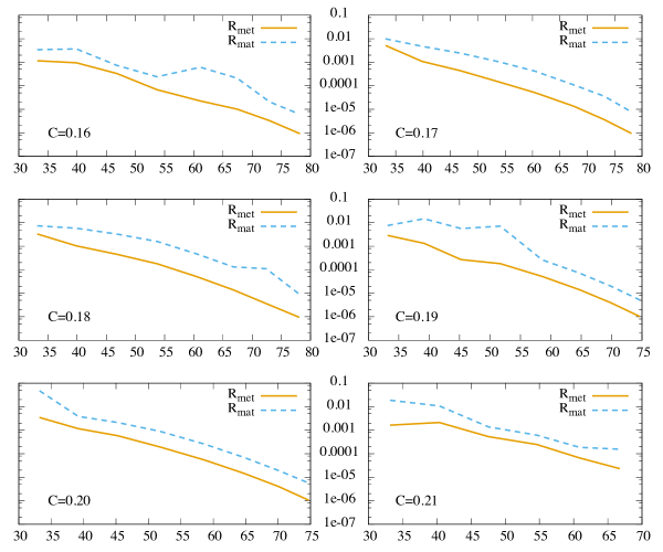
Figure 2: Spectral convergence for a family of BHNS binary configurations. For each configuration, the equation of state is a $\Gamma=2$ polytrope chosen to yield $M_{\mathrm{NS}}=$1.4\text{\,}\text{M_\odot}$$. Each panel shows the final residual in the metric solution ($R_{\mathrm{met}}$) and in the velocity potential solution ($R_{\mathrm{mat}}$) as a function of the cube root of the number of grid points in the domain. The vertical scale is logarithmic, and the exponential convergence with resolution is apparent.

III.2 SLy $\mathbf{\Gamma\boldsymbol{=}2}$ EOS

Using the methods of this paper, we can obtain solutions for an SLy equation of state with compactness up to $\mathcal{C}=0.25$, which corresponds to a star with a mass of $1.86\text{\,}\text{$M_{\odot}$}$. For comparison, the maximum stable compactness for this equation of state is about $\mathcal{C}=0.31$, corresponding to a mass of $2.04\text{\,}\text{$M_{\odot}$}$. Solutions were found for a variety of different distances, although as the compactness becomes greater, it becomes more difficult to obtain solutions for very close binaries. At the highest compactness, the closest binaries we attempted did not have a convergent solution, and so an evolution of such a system would need to simulate more than 20 orbits before a merger.

These results are shown in Table 2. The mass ratio $q$ is close to 6, with slight variations between solutions. The residuals obtained in the solve are shown in Fig. 3, plotted against $N^{1/3}$, the cube root of the number of points in the domain. Note that for the $\mathcal{C}=0.23$ and $\mathcal{C}=0.25$ cases, we have only plotted the convergence in the case of $d=14M_{0}$. Even more so than in the polytropic case, there are some jumps in the residuals, particularly in the velocity potential. Furthermore, jumps are present at all compactnesses instead of just low ones. However, once again, the convergence does appear smoothly exponential at high resolution. The same value for the relaxation parameter is used for all of the various quantities that are updated via a relaxation scheme.

$\mathcal{C}$	$M_{\mathrm{NS}}$	$q$	$\lambda$	$d/M_{0}$	$\Omega M_{0}$	$E_{b}/M_{0}$	$J/{M_{0}}^{2}$	$S_{20}/S_{00}$
0.16	1.27	6.64	0.2	6.95	0.04560	-6.15	0.393	4.928
0.17	1.34	6.26	0.2	6.90	0.04611	-6.46	0.409	4.696
0.18	1.41	5.94	0.2	6.85	0.04659	-6.77	0.424	4.460
0.19	1.49	5.65	0.2	6.80	0.04707	-7.05	0.438	4.231
0.21	1.62	6.0	0.15	13.71	0.01791	-3.91	0.522	1.533
0.23	1.75	6.0	0.15	8.0	0.03785	-6.05	0.438	2.878
0.23	1.75	6.0	0.15	10.0	0.02785	-5.09	0.468	2.066
0.23	1.75	6.0	0.15	12.0	0.02160	-4.39	0.497	1.611
0.23	1.75	6.0	0.15	14.0	0.01739	-3.82	0.526	1.324
0.23	1.75	6.0	0.15	16.0	0.01439	-3.22	0.552	1.124
0.25	1.86	6.0	0.1	14.0	0.01738	-3.88	0.525	1.144
0.25	1.86	6.0	0.1	16.0	0.01438	-2.38	0.552	0.971
						$\times 10^{-3}$		$\times 10^{-3}$

Table 2: Solved quantities for a family of BHNS binary configurations. For each configuration, the equation of state is SLy. The multiplier below applies to the column above it. The quantities shown are all as for Table 1, with $\kappa$ replaced by the neutron star ADM mass $M_{\mathrm{NS}}$ in units of $M_{\odot}$. We also show the mass ratio $q$ for each configuration.

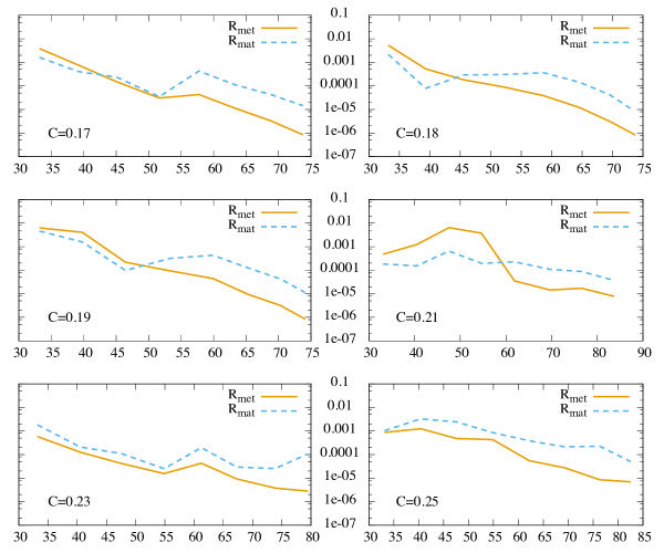
Figure 3: Spectral convergence for a family of BHNS binary configurations. For each configuration, the equation of state is SLy. Each panel shows the final residual in the metric solution ($R_{\mathrm{met}}$) and in the velocity potential solution ($R_{\mathrm{mat}}$) as a function of the cube root of the number of grid points in the domain. The vertical scale is logarithmic, and the exponential convergence with resolution is apparent.

III.3 LS220 EOS

We obtain solutions for an LS220 tabulated equation of state with compactness up to $\mathcal{C}=0.26$, which corresponds to a star with a mass of $1.98\text{\,}\text{$M_{\odot}$}$. For comparison, the largest known reliable neutron star masses are $1.97\pm 0.04\text{\,}\text{$M_{\odot}$}$ Demorest et al. (2010) and $2.01\pm 0.04\text{\,}\text{$M_{\odot}$}$ Antoniadis et al. (2013). The LS220 equation of state is the most realistic of the ones considered here, and so this is a very relevant result. The largest compactness for which this equation of state yields a stable solution is $\mathcal{C}=0.29$, corresponding to a mass of $2.04\text{\,}\text{$M_{\odot}$}$.

These results are shown in Table 3. In all cases, the mass ratio is 6:1. The residuals obtained in the solve are shown in Fig. 4, plotted against $N^{1/3}$, the cube root of the number of points in the domain. As before, we find exponential convergence, and obtain a final residual of ${10}^{-6}$ or nearly so.

$\mathcal{C}$	$M_{\mathrm{NS}}$	$\lambda$	$d/M_{0}$	$\Omega M_{0}$	$E_{b}/M_{0}$	$J/{M_{0}}^{2}$	$S_{20}/S_{00}$
0.17	1.40	0.2	14.0	0.01739	-3.84	0.526	1.885
0.23	1.83	0.1	14.0	0.01739	-3.83	0.526	1.347
0.25	1.94	0.08	16.0	0.01439	-3.18	0.552	0.985
0.26	1.98	0.07	14.0	0.01739	-3.73	0.525	1.075
					$\times 10^{-3}$		$\times 10^{-3}$

Table 3: Solved quantities for a family of BHNS binary configurations. For each configuration, the equation of state is the LS220 tabulated equation of state. The multiplier below applies to the column above it. The quantities shown are all as for Table 1, with $\kappa$ replaced by the neutron star ADM mass $M_{\mathrm{NS}}$ in units of $M_{\odot}$.

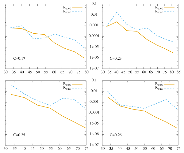
Figure 4: Spectral convergence for a family of BHNS binary configurations. For each configuration, the equation of state is LS220. Each panel shows the final residual in the metric solution ($R_{\mathrm{met}}$) and in the velocity potential solution ($R_{\mathrm{mat}}$) as a function of the cube root of the number of grid points in the domain. The vertical scale is logarithmic, and the exponential convergence with resolution is apparent.

IV Conclusions

The problem of solving for initial data for a black hole–neutron star system is a complex one involving many interacting solution steps. In addition to the elliptic equations governing the system, multiple nonlinear constraints must be imposed simultaneously. In this paper, we focused on two of these in particular: aligning the surface with a subdomain boundary and enforcing zero linear momentum on the binary system. The close interaction between the equations and all of the constraints requires care in solving the system, and for some choices of system parameters the convergence of the system can be very sensitive to deficiencies in the solution method. In fact, it seems to be generally true that high compactness stars cause difficulty with the various solvers that exist.

We have found that by applying additional relaxation steps to the method of Paper I Foucart et al. (2008) we could obtain solutions for a wide variety of systems with quite high compactness stars, including stars with polytropic, SLy, and LS220 equations of state. This includes a solution for a binary with a physically realistic LS220 equation of state star having a mass of $M=$1.98\text{\,}\text{M_\odot}$$. We have found it effective to employ a relaxation scheme in updating the metric and velocity potential quantities from the elliptic solver procedure, as well as the neutron star surface location, in addition to a boost parameter in a control scheme adjusting for undesired linear ADM momentum in the system. The choice of different relaxation parameters allows one to tune the solver for the convergence properties of the particular solution being examined. These improvements allow solutions to the black hole–neutron star initial data problem to be found for physically important cases.