Phase transition for large dimensional contact process with random recovery rates on open clusters

Abstract: In this paper we are concerned with contact process with random recovery rates on open clusters of bond percolation on $\mathbb{Z}^{d}$. Let $\xi$ be a positive random variable, then we assigned i. i. d. copies of $\xi$ on the vertices as the random recovery rates. Assuming that each edge is open with probability $p$ and $\log d$ vertices are occupied at $t=0$, we prove that the following phase transition occurs. When the infection rate $\lambda<\lambda_{c}=1/({p{\rm E}\frac{1}{\xi}})$, then the process dies out at time $O(\log d)$ with high probability as $d\rightarrow+\infty$, while when $\lambda>\lambda_{c}$, the process survives with high probability.

Keywords: contact process, random recovery rates, percolation, phase transition.

1 Introduction

In this paper, we are concerned with contact process with random recover rates on open clusters of bond percolation in lattice. First we introduce some notations. For each $d\geq 1$, we denote by $\mathbb{Z}^{d}$ the $d$-dimensional lattice and denote by $\mathbb{E}^{d}$ the set of edges on $\mathbb{Z}^{d}$. For any $x,y\in\mathbb{Z}^{d}$, we denote by $x\sim y$ when there exits $e\in\mathbb{E}^{d}$ connecting $x$ and $y$. Let $\{X(e)\}_{e\in\mathbb{E}^{d}}$ be i. i. d. random variables such that

$$P(X(e)=1)=p=1-P(X(e)=0)$$ (1.1)

for each $e\in\mathbb{E}^{d}$, where $p\in(0,1)$, then we denote by $x\leftrightarrow y$ when and only when $x\sim y$ and the edge $e$ connecting $x$ and $y$ satisfies that $X(e)=1$. For each $x\in\mathbb{Z}^{d}$, we define

$$\mathcal{N}(x)=\{y:y\leftrightarrow x\}$$ (1.2)

as the set of neighbors of $x$. Please note that $\mathcal{N}(x)$ is a random set depending on $\{X(e)\}_{e\in\mathbb{E}^{d}}$. Let $\xi$ be a random variable such that $P(\xi\geq 1)=1$ and $\{\xi(x)\}_{x\in\mathbb{Z}^{d}}$ be i. i. d. random variables such that $\xi(x)$ and $\xi$ have identical probability distributions. We assume that $\{\xi(x)\}_{x\in\mathbb{Z}^{d}}$ and $\{X(e)\}_{e\in\mathbb{E}^{d}}$ are independent.

The contact process is a Markov process with state space

$$\mathcal{P}(\mathbb{Z}^{d})=\{A:A\subseteq\mathbb{Z}^{d}\}.$$

For any $t\geq 0$, we denote by $C_{t}$ the state of the process at the moment $t$. After $\{X(e)\}_{e\in\mathbb{E}^{d}}$ and $\{\xi(x)\}_{x\in\mathbb{Z}^{d}}$ are given, $\{C_{t}\}_{t\geq 0}$ evolves as follows.

$$C_{t}\rightarrow\begin{cases}C_{t}\setminus\{x\}\text{~{}at rate~{}}\xi(x)&\text{\quad if~{}}x\in C_{t},\\ C_{t}\cup\{x\}\text{~{}at rate~{}}\frac{\lambda}{2d}|\mathcal{N}(x)\cap C_{t}|&\text{\quad if~{}}x\not\in C_{t},\end{cases}$$ (1.3)

where $\lambda$ is a positive parameter called the infection rate.

The contact process describes the spread of an infection disease on $\mathbb{Z}^{d}$. Vertices in $C_{t}$ are infected while vertices out of $C_{t}$ are healthy. An infected vertex $x$ waits for an exponential time with rate $\xi(x)$ to become healthy. An healthy vertex $y$ is infected at rate proportional to the number of infected neighbors.

When $p=1$ and $P(\xi=1)=1$, the model turns into the classic contact process introduced by Harris in [4]. The two books [9] and [11] authored by Liggett give a detailed survey of the study of contact process.

In recent years, the contact process on random graph generated from the percolation model is a popular topic. In [1], Bertacchi, Lanchier and Zucca study the contact process on $C_{\infty}\times K_{N}$, where $C_{\infty}$ is the infinite open cluster of the site percolation and $K_{N}$ is the complete graph with $N$ vertices. They give criterions to judge whether the process will die out. In [3], Chen and Yao show that the complete convergence theorem holds for contact process on open clusters of $\mathbb{Z}^{d}\times\mathbb{Z}^{+}$. In [13], Xue shows that the contact process on open clusters of oriented bond percolation in $\mathbb{Z}^{d}$ has critical value approximately $1/(dp)$ as $d$ grows to infinity, where $p$ is the probability that an given edge is open.

The study of contact process with random recovery rates dates back to 1980s. In [2], Bramson, Durrett and Schonmann show that the contact process with random recovery rates on $\mathbb{Z}^{1}$ has an ‘intermediate phase’ in which the process survives but does not grow linearly. In [10], Liggett studies contact process with random recovery rates and random infection rates on $\mathbb{Z}^{1}$ and gives a sufficient condition for the process to survive.

2 Main results

In this section we give main results of this paper. First we introduce some definition and notations. For $d\geq 1$, we assume that $\{X(e)\}_{e\in\mathbb{E}^{d}}$ and $\{\xi(x)\}_{x\in\mathbb{Z}^{d}}$ are defined under a probability space $(\Omega_{d},\mathcal{F}_{d},\mu_{d})$. The expectation operator with respect to $\mu_{d}$ is denoted by ${\rm E}_{\mu_{d}}$. For any $\omega\in\Omega_{d}$ and $\lambda>0$, we denote by $P_{\lambda}^{\omega}$ the probability measure of the contact process $\{C_{t}\}_{t\geq 0}$ with infection rate $\lambda$ and recovery rates $\{\xi(\omega,x)\}_{x\in\mathbb{Z}^{d}}$ on open clusters generated from $\{X(\omega,e)\}_{e\in\mathbb{E}^{d}}$. $P_{\lambda}^{\omega}$ is called the quenched measure. The expectation operator with respect to $P_{\lambda}^{\omega}$ is denoted by ${\rm E}_{\lambda}^{\omega}$. For each $d\geq 1$, we define

$$P_{\lambda,d}(\cdot)=\int P_{\lambda}^{\omega}(\cdot)~{}\mu_{d}(d\omega)={\rm E}_{\mu_{d}}[P_{\lambda}^{\omega}(\cdot)],$$

which is called the annealed measure. The expectation operator with respect to $P_{\lambda,d}$ is denoted by ${\rm E}_{\lambda,d}$. When there is no misunderstanding, we write $P_{\lambda,d}$ and ${\rm E}_{\lambda,d}$ as $P_{\lambda}$ and $E_{\lambda}$. For any $A\subseteq\mathbb{Z}^{d}$, we write $C_{t}$ as $C_{t}^{A}$ when $C_{0}=A$.

Now we can give our main result.

Theorem 2.1.

For each $d\geq 1$, let $A(d)$ be a subset of $\mathbb{Z}^{d}$ such that $|A(d)|=\lceil\log d\rceil$, then for any $\lambda<\lambda_{c}=1/(p{\rm E}\frac{1}{\xi})$, there exists $c(\lambda)>0$ such that

$$\lim_{d\rightarrow+\infty}P_{\lambda,d}(C_{c(\lambda)\log d}^{A(d)}\neq\emptyset)=0,$$ (2.1)

while for any $\lambda>\lambda_{c}$,

$$\lim_{d\rightarrow+\infty}P_{\lambda,d}(\forall~{}t>0,C_{t}^{A(d)}\neq\emptyset)=1.$$ (2.2)

According to Theorem 2.1, phase transition occurs when the infection rate $\lambda$ grows from $\lambda<\lambda_{c}$ to $\lambda>\lambda_{c}$, where

$$\lambda_{c}=1/(p{\rm E}\frac{1}{\xi}).$$

We denote by $O$ the origin of $\mathbb{Z}^{d}$. According to the basic coupling of spin systems (See Section 3.1 of [9]), it is easy to see that for any $\lambda_{1}\geq\lambda_{2}$

$$P_{\lambda_{1}}(\forall~{}t>0,C_{t}^{O}\neq\emptyset)\geq P_{\lambda_{2}}(\forall~{}t>0,C_{t}^{O}\neq\emptyset).$$

Therefore, for each $d\geq 1$, the following definition is reasonable.

$$\lambda_{d}=\sup\{\lambda:P_{\lambda,d}(\forall~{}t>0,C_{t}^{O}\neq\emptyset)=0\}.$$ (2.3)

According to Theorem 2.1, we have the following corollary.

Corollary 2.2.

$\lambda_{d}$ is as that defined in (2.3), then

$$\limsup_{d\rightarrow+\infty}\lambda_{d}\leq\lambda_{c}=1/(p{\rm E}\frac{1}{\xi}).$$

When $p=\xi=1$, Corollary 2.2 shows that $\limsup_{d\rightarrow+\infty}\lambda_{d}\leq 1$. A stronger conclusion such that $\lim_{d\rightarrow+\infty}\lambda_{d}=1$ for the classic contact process is shown by Holley and Liggett in [6]. In [12], Xue shows that the critical value of high dimensional threshold one contact process has similar asymptotic behavior.

The proof of Theorem 2.1 is divided into two sections. In Section 3, we will prove Equation (2.1). The proof is inspired by the approach of graphical representation introduced by Harris in [5]. In Section 4, we will prove Equation (2.2). The proof is inspired by the approach introduced by Kesten in [8] to study the asymptotic behavior of the critical probability of high dimensional percolation model.

3 Subcritical case

In this section we give the proof of (2.1). First we introduce the graphical representation of the process $\{C_{t}\}_{t\geq 0}$. We consider the graph $\mathbb{Z}^{d}\times[0,+\infty)$. In other words, we erect a time arrow on each vertex on $\mathbb{Z}^{d}$. After $\{\xi(x)\}_{x\in\mathbb{Z}^{d}}$ and $\{X(e)\}_{e\in\mathbb{E}^{d}}$ are given, we assume that $\{Y_{x}(t)\}_{t\geq 0}$ is a Poisson process with rate $\xi(x)$ and $\{U_{(x,y)}(t)\}_{t\geq 0}$ is a Poisson process with rate $\lambda/(2d)$ for each $x,y\in\mathbb{Z}^{d},x\sim y$. We assume that all these Poisson processes are independent. Please note that we care about the order of $x$ and $y$, hence $U_{(x,y)}\neq U_{(y,x)}$. For any event time $t$ of $Y_{x}$, we put a ‘$\Delta$’ at $(x,t)$. For any event time $s$ of $U_{(x,y)}$, we put an arrow ‘$\rightarrow$’ from $(x,s)$ to $(y,s)$. For $x,y\in\mathbb{Z}^{d}$ and $t>0$, we say that there is an infection path from $(x,0)$ to $(y,t)$ when there exist $x=x_{0}\sim x_{1}\sim x_{2}\sim\ldots\sim x_{n}=y$ and $0=t_{-1}<t_{0}<t_{1}<\ldots<t_{n}=t$ satisfying all the following three conditions.

(1) For $0\leq i\leq n-1$, there is an arrow from $(x_{i},t_{i})$ to $(x_{i+1},t_{i})$.

(2) For $0\leq i\leq n$, there is no ‘$\Delta$’ on $\{x_{i}\}\times(t_{i-1},t_{i}]$.

(3) For $0\leq i\leq n-1$, $X(x_{i},x_{i+1})=1$.

Please note that we write $X(e)$ as $X(x,y)$ when $e$ connecting $x$ and $y$. The following figure gives an example of infection path.

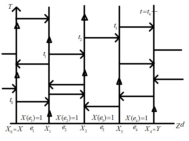
Figure 1: Infection path

In Figure 1, there is an infection path from $(x_{0},0)$ to $(x_{4},t)$. According to the transition rates function of $\{C_{t}\}_{t\geq 0}$ given by (1.3), it is easy to see that

$$C_{t}^{A}=\{y:\text{~{}for some~{}}x\in A,\text{~{}there is an infection path from~{}}(x,0)\text{~{}to~{}}(y,t)\}$$ (3.1)

for any $A\subseteq\mathbb{Z}^{d}$ in the sense of coupling. By Equation (3.1),

$$C_{t}^{A}=\cup_{x\in A}C_{t}^{x}$$

in the sense of coupling. Therefore, for any finite $A$,

$$P_{\lambda}^{\omega}(C_{t}^{A}\neq\emptyset)\leq\sum_{x\in A}P_{\lambda}^{\omega}(C_{t}^{x}\neq\emptyset)$$ (3.2)

and

$$P_{\lambda,d}(C_{t}^{A}\neq\emptyset)\leq|A|P_{\lambda,d}(C_{t}^{O}\neq\emptyset).$$ (3.3)

For later use, we divided the infection paths into several types. For each $n\geq 0$, we define

$$B_{n}=\{(x_{0},x_{1},x_{2},\ldots,x_{n}):O=x_{0}\sim x_{1}\sim x_{2}\sim\ldots\sim x_{n}\}$$

as the set of path starting at $O$ with length $n$. For $\vec{x}=(O,x_{1},x_{2},\ldots,x_{n})\in B_{n}$ and $n$ positive integers $j_{0},j_{1},\ldots,j_{n-1}$, we say that $\vec{x}$ is an infection path with type $(j_{0},j_{1},\ldots,j_{n-1})$ at the moment $t$ when there exists $0=t_{-1}<t_{0}<t_{1}<\ldots<t_{n}=t$ such that

(1) For $0\leq i\leq n-1$, there is an arrow from $(x_{i},t_{i})$ to $(x_{i+1},t_{i})$.

(2) For $0\leq i\leq n$, there is no ‘$\Delta$’ on $\{x_{i}\}\times(t_{i-1},t_{i}]$.

(3) For $0\leq i\leq n-1$, $X(x_{i},x_{i+1})=1$.

(4) For $0\leq i\leq n-1$, $t_{i}$ is the $j_{i}$th event time of $U_{(x_{i},x_{i+1})}$ after the moment $t_{i-1}$.

The following figure gives an example.

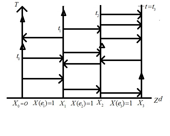
Figure 2: Infection path type

In Figure 2, $(O,x_{1},x_{2},x_{3})$ is an infection path with type $(2,2,2)$ at the moment $t$. Please note that an infection path may be with more than one type. In Figure 2, $(O,x_{1},x_{2},x_{3})$ is also with the type $(2,2,1)$. We use $A(\vec{x},j_{0},j_{1},\ldots,j_{n-1},t)$ to denote the event that $\vec{x}$ is an infection path with type $(j_{0},j_{1},\ldots,j_{n-1})$ at the moment $t$. We define

$$A(\vec{x},t)=\bigcup_{j_{0},j_{1},\ldots,j_{n-1}}A(\vec{x},j_{0},j_{1},\ldots,j_{n-1},t)$$

as the vent that $\vec{x}$ is an infection path at the moment $t$. For later use, we define

$$D_{n}=\{\vec{x}=(x_{0},x_{1},\ldots,x_{n})\in B_{n}:x_{i}\neq x_{j}\text{~{}for any~{}}0\leq i<j\leq n\}.$$

After all the above prepared work, we give the proof of Equation (2.1).

Proof of Equation 2.1.

We let $c(\lambda)=\frac{1}{2\lambda}$ and $t=c(\lambda)\log d$. By Equation (3.1),

$$P_{\lambda,d}(C_{t}^{O}\neq\emptyset)\leq \sum_{n=0}^{+\infty}\sum_{\vec{x}\in D_{n}}\sum_{j_{0},j_{1},\ldots,j_{n-1}\geq 1}P_{\lambda,d}\big{(}A(\vec{x},j_{0},\ldots,j_{n-1},t)\big{)}$$ (3.4)

$$+\sum_{n=0}^{+\infty}\sum_{\vec{x}\in B_{n}\setminus D_{n}}P_{\lambda,d}\big{(}A(\vec{x},t)\big{)}.$$

First we deal with $\sum_{n=0}^{+\infty}\sum_{\vec{x}\in B_{n}\setminus D_{n}}P_{\lambda,d}\big{(}A(\vec{x},t)\big{)}$ .It is easy to see that $B_{n}=D_{n}$ for $n=0,1$, hence

$$\sum_{n=0}^{+\infty}\sum_{\vec{x}\in B_{n}\setminus D_{n}}P_{\lambda,d}\big{(}A(\vec{x},t)\big{)}=\sum_{n=2}^{+\infty}\sum_{\vec{x}\in B_{n}\setminus D_{n}}P_{\lambda,d}\big{(}A(\vec{x},t)\big{)}.$$ (3.5)

For each $n\geq 2$, it is easy to see that

$$|B_{n}\setminus D_{n}|\leq{n+1\choose 2}(2d)^{n-1}.$$ (3.6)

This is because for any $\vec{x}\in B_{n}\setminus D_{n}$, there exists $i\neq j$ such that $x_{i}=x_{j}$ and for each $l\neq 0,i,j$, $x_{l}$ has at most $2d$ choices. Let $\{N(s)\}_{s\geq 0}$ be a Poison process with rate $\frac{\lambda}{2d}$, then we claim that

$$P_{\lambda,d}(A(\vec{x},t))\leq P(N(t)\geq n)$$ (3.7)

for each $\vec{x}\in B_{n}\setminus D_{n}$. To explain (3.7), we denote $T_{0}$ the first event time of $U_{(x_{0},x_{1})}$ and $T_{l}$ the first event time of $U_{(x_{l},x_{l+1})}$ after the moment $T_{l-1}$ for $1\leq l\leq n-1$. Therefore, $\{T_{j}-T_{j-1}\}_{0\leq j\leq n-1}$ are i. i. d. exponential times with rate $\frac{\lambda}{2d}$, where $T_{-1}=0$. As a result,

$$P(T_{n-1}<t)=P(N(t)\geq n).$$ (3.8)

If $\vec{x}$ is an infection path at the moment $t$, then there exists $t_{0}<t_{1}<\ldots<t_{n-1}<t_{n}=t$ such that $t_{i}$ is an event time of $U_{(x_{i},x_{i+1})}$ at which $x_{i}$ infects $x_{i+1}$. According to the definition of $\{T_{j}\}_{0\leq j\leq n-1}$,

$$T_{j}\leq t_{j}$$

for each $1\leq j\leq n-1$. As a result,

$$P_{\lambda,d}(A(\vec{x},t))\leq P_{\lambda,d}(T_{n-1}<t).$$ (3.9)

Equation (3.7) follows from (3.8) and (3.9).

For $\theta>0$,

$$P(N(t)\geq n)\leq e^{-\theta n}{\rm E}e^{\theta N(t)}=e^{\frac{\lambda t}{2d}(e^{\theta}-1)-\theta n}.$$

For sufficiently large $d$, $n\geq 2$ and $t=\frac{1}{2\lambda}\log d$, we choose $\theta=\log\frac{2dn}{\lambda t}$, then according to the Stirling’s Formula,

$$P(N(t)\geq n)\leq\frac{e^{n}e^{-\frac{\lambda t}{2d}}(\lambda t)^{n}}{(2dn)^{n}}\leq\frac{M\sqrt{n}}{n!}\big{(}\frac{\lambda t}{2d}\big{)}^{n},$$ (3.10)

where $M$ is a constant which does not depend on $\lambda,t,d$ and $n$.

By Equation (3.5), (3.6), (3.7) and (3.10), when $t=\frac{1}{2\lambda}\log d$,

$$\sum_{n=0}^{+\infty}\sum_{\vec{x}\in B_{n}\setminus D_{n}}P_{\lambda,d}\big{(}A(\vec{x},t)\big{)} \leq M\sum_{n=2}^{+\infty}\frac{(n+1)n(2d)^{n-1}\sqrt{n}}{2n!}\big{(}\frac{\lambda t}{2d}\big{)}^{n}$$

$$\leq\frac{M_{1}}{2d}\sum_{n=2}^{+\infty}\frac{n^{3}(\lambda t)^{n}}{n!}$$

$$\leq\frac{M_{2}(\lambda t)^{2}+M_{3}(\lambda t)^{3}e^{\lambda t}}{2d}$$

$$=\frac{M_{4}\log^{2}d}{d}+\frac{M_{5}\log^{3}d}{\sqrt{d}}$$ (3.11)

where $M_{1},M_{2},M_{3},M_{4},M_{5}$ are constant does not depend on $\lambda,t,n$ and $d$.

Now we deal with $P_{\lambda,d}(A(\vec{x},j_{0},j_{1},\ldots,j_{n-1},t))$ for $\vec{x}\in D_{n}$. For given $\omega\in\Omega_{d}$, we let $S_{0},S_{1},\ldots,S_{n-1}$ be independent exponential times with rates $\xi(x_{0},\omega),\xi(x_{1},\omega),\ldots,\xi(x_{n},\omega)$ respectively. We let $\{W_{i}\}_{1\leq i\leq+\infty}$ be i. i. d. exponential times with rate $\frac{\lambda}{2d}$ and $\{V_{m}\}_{0\leq m\leq n-1}$ be independent random variables such that $V_{m}$ and $\sum_{l=1}^{j_{m}}W_{l}$ have identical probability distributions for $0\leq m\leq n-1$. Then, according to the definition of $A(\vec{x},j_{0},j_{1},\ldots,j_{n-1},t)$,

$$P_{\lambda}^{\omega}(A(\vec{x},j_{0},j_{1},\ldots,j_{n-1},t))$$

$$=p^{n}P(\sum_{m=0}^{n-1}V_{m}\leq t,S_{m}\geq V_{m},0\leq m\leq n-1,S_{n}\geq t-\sum_{m=0}^{n-1}V_{m}).$$ (3.12)

Please note that the factor $p^{n}$ in Equation (3) is the probability that $X(x_{i},x_{i+1})=1$ for $0\leq i\leq n-1$, since $\{X(x_{i},x_{i+1})\}_{0\leq i\leq n-1}$ are i. i. d. for $\vec{x}=(x_{0},x_{1},\ldots,x_{n})\in D_{n}\texttt{{}}$.

Since

$$P(S_{m}\geq V_{m}|V_{0},\ldots,V_{n-1})=e^{-\xi(x_{m})V_{m}}$$

and $V_{m}$ has probability density

$$p(t_{m},j_{m})=\frac{t_{m}^{j_{m}-1}e^{-\frac{\lambda}{2d}t_{m}}}{(j_{m}-1)!}(\frac{\lambda}{2d})^{j_{m}}$$

for $0\leq m\leq n-1$,

$$P_{\lambda}^{\omega}(A(\vec{x},j_{0},j_{1},\ldots,j_{n-1},t))$$

$$=p^{n}\int\limits_{\sum_{m=0}^{n-1}t_{m}\leq t}\prod_{m=0}^{n-1}p(t_{m},j_{m})e^{-\sum\limits_{m=0}^{n-1}\xi(x_{m})t_{m}}e^{-\xi(x_{n})(t-\sum\limits_{m=0}^{n-1}t_{m})}~{}dt_{0}~{}dt_{1}...~{}dt_{m}.$$ (3.13)

By Equation (3) and direct calculation, it is not difficult to check that

$$\sum\limits_{j_{0},\ldots,j_{n-1}\geq 1}P_{\lambda}^{\omega}(A(\vec{x},j_{0},j_{1},\ldots,j_{n-1},t))$$

$$=(\frac{\lambda p}{2d})^{n}\int\limits_{\sum\limits_{m=0}^{n-1}t_{m}\leq t}e^{-\sum\limits_{m=0}^{n-1}\xi(x_{m})t_{m}}e^{-\xi(x_{n})(t-\sum\limits_{m=0}^{n-1}t_{m})}~{}dt_{0}~{}dt_{1}\ldots~{}dt_{n-1}$$

$$=(\frac{\lambda p}{2d})^{n}\frac{1}{\prod\limits_{m=0}^{n-1}\xi(x_{m})}P(\sum\limits_{m=0}^{n-1}S_{m}\leq t,S_{n}\geq t-\sum_{m=0}^{n-1}t_{m}).$$ (3.14)

The calculation is a little tedious, we omit the details. Let $\{\alpha(t)\}_{t\geq 0}$ be a Poison process with rate $1$, then

$$P(\sum\limits_{m=0}^{n-1}S_{m}\leq t,S_{n}\geq t-\sum_{m=0}^{n-1}S_{m})\leq P(\sum\limits_{m=0}^{n}S_{m}\geq t)\leq P(\alpha(t)\leq n+1),$$ (3.15)

since $\xi(x)\geq 1$ for each $x\in\mathbb{Z}^{d}$. By Equation (3) and (3.15),

$$\sum_{n=0}^{+\infty}\sum_{\vec{x}\in D_{n}}\sum_{j_{0},j_{1},\ldots,j_{n-1}\geq 1}P_{\lambda,d}\big{(}A(\vec{x},j_{0},\ldots,j_{n-1},t)\big{)}$$

$$\leq\sum_{n=0}^{+\infty}\sum_{\vec{x}\in D_{n}}(\frac{\lambda p}{2d})^{n}{\rm E}_{\mu_{d}}\Big{[}\frac{1}{\prod\limits_{m=0}^{n-1}\xi(x_{m})}\Big{]}P(\alpha(t)\leq n+1).$$ (3.16)

For $\vec{x}\in D_{n}$, $\{x_{i}\}_{0\leq i\leq n}$ are different with each other, therefore

$${\rm E}_{\mu_{d}}\Big{[}\frac{1}{\prod\limits_{m=0}^{n-1}\xi(x_{m})}\Big{]}=({\rm E\frac{1}{\xi}})^{n}.$$ (3.17)

Since each vertex on $\mathbb{Z}^{d}$ has $2d$ neighbors,

$$|D_{n}|\leq(2d)^{n}.$$ (3.18)

By Equation (3), (3.17) and (3.18),

$$\sum_{n=0}^{+\infty}\sum_{\vec{x}\in D_{n}}\sum_{j_{0},j_{1},\ldots,j_{n-1}\geq 1}P_{\lambda,d}\big{(}A(\vec{x},j_{0},\ldots,j_{n-1},t)\big{)}\leq\sum_{n=0}^{+\infty}(\lambda p{\rm E}\frac{1}{\xi})^{n}P(\alpha(t)\leq n+1).$$ (3.19)

For $n\leq\lfloor\frac{1}{4\lambda}\log d\rfloor-1$,

$$P(\alpha(t)\leq n+1)\leq P(\alpha(t)\leq t/2)\leq 2^{\frac{t}{2}}{\rm E}(\frac{1}{2})^{\alpha(t)}=(\sqrt{\frac{2}{e}})^{t}.$$ (3.20)

By Equation (3.19) and (3.20), when $\lambda<\lambda_{c}$,

$$\sum_{n=0}^{+\infty}\sum_{\vec{x}\in D_{n}}\sum_{j_{0},j_{1},\ldots,j_{n-1}\geq 1}P_{\lambda,d}\big{(}A(\vec{x},j_{0},\ldots,j_{n-1},t)\big{)}$$

$$\leq\lfloor\frac{1}{4\lambda}\log d\rfloor(\sqrt{\frac{2}{e}})^{t}+\sum\limits_{n=\lfloor\frac{1}{4\lambda}\log d\rfloor}^{+\infty}(\lambda p{\rm E}\frac{1}{\xi})^{n}$$

$$=\lfloor\frac{1}{4\lambda}\log d\rfloor\big{[}(\frac{2}{e})^{\frac{1}{4\lambda}}\big{]}^{\log d}+\frac{(\lambda p{\rm E}\frac{1}{\xi})^{\lfloor\frac{1}{4\lambda}\log d\rfloor}}{1-\lambda p{\rm E}\frac{1}{\xi}}.$$ (3.21)

By Equation (3.4), (3) and (3), when $\lambda<\lambda_{c}$,

$$\lim_{d\rightarrow+\infty}(\log d)P_{\lambda,d}(C_{\frac{1}{2\lambda}\log d}^{O}\neq\emptyset)=0.$$ (3.22)

Equation (2.1) follows from Equation (3.3) and (3.22) with $c(\lambda)=\frac{1}{2\lambda}$.

∎

4 Supcritical case

In this section we give the proof of Equation (2.2). Our proof is inspired by a technique introduced in [8], where $\lim_{d\rightarrow+\infty}2dp_{c}(d)=1$ is shown for the critical probability $p_{c}(d)$ of $d$-dimensional site percolation. First we introduce some notations. For each $d\geq 1$, we define

$$N(d)=\lfloor\frac{\log d}{2\log\log d}\rfloor.$$

We write $N(d)$ as $N$ when there is no misunderstanding. For $1\leq i\leq d$, we define

$$e_{i}=(0,~{}\ldots,~{}0,\mathop{1}\limits_{i\text{th}},0,~{}\ldots,~{}0).$$

For $x\in\mathbb{Z}^{d}$ and integer $k\geq 1$, we define

$$F_{k}(x)= \Big{\{}\vec{x}=(x_{0},x_{1},\ldots,x_{kN-1}):x=x_{0}\sim x_{1}\sim\ldots\sim x_{kN-1},\text{~{}for~{}}N|(j+1),$$

$$x_{j+1}-x_{j}\in\{e_{k}:k>d-\lfloor\frac{d}{N}\rfloor\},\text{~{}for~{}}N\not|(j+1),$$ (4.1)

$$x_{j+1}-x_{j}\in\{\pm e_{k}:k\leq d-\lfloor\frac{d}{N}\rfloor\}\Big{\}}.$$

For each $\vec{x}\in F_{k}(x)$, we denote by $I_{k}(\vec{x})$ the event that there exists $t>0$ such that $\vec{x}$ is an infection path with type $(1,1,\ldots,1)$ at the moment $t$. On the event $\bigcap\limits_{k=1}^{+\infty}\bigcup\limits_{x\in A}\bigcup\limits_{\vec{x}\in F_{k}(x)}I_{k}(\vec{x})$, there exists infection path starting at some vertex in $A$ and ending at vertex with arbitrary large norm, hence the process will not die out. Therefore,

$$P_{\lambda,d}(C_{t}^{A}\neq\emptyset,\forall~{}t>0) \geq P_{\lambda,d}\Big{(}\bigcap\limits_{k=1}^{+\infty}\bigcup\limits_{x\in A}\bigcup\limits_{\vec{x}\in F_{k}(x)}I_{k}(\vec{x})\Big{)}$$

$$=\lim\limits_{k\rightarrow+\infty}P_{\lambda,d}\Big{(}\bigcup\limits_{x\in A}\bigcup\limits_{\vec{x}\in F_{k}(x)}I_{k}(\vec{x})\Big{)}.$$ (4.2)

To deal with $P_{\lambda,d}\Big{(}\bigcup\limits_{x\in A}\bigcup\limits_{\vec{x}\in F_{k}(x)}I_{k}(\vec{x})\Big{)}$ later, we need the following lemma.

Lemma 4.1.

Suppose that $A_{1},A_{2},\ldots,A_{n}$ are some random events under an identical probability space such that $P(A_{i})>0$ for $1\leq i\leq n$, then

$$P\big{(}\bigcup\limits_{i=1}^{n}A_{i}\big{)}\geq\frac{1}{\frac{1}{n^{2}}\sum\limits_{i=1}^{n}\sum\limits_{j=1}^{n}\frac{P(A_{i}\bigcap A_{j})}{P(A_{i})P(A_{j})}}.$$

Proof.

For $1\leq i\leq n$, we define $Y_{i}=\frac{1_{A_{i}}}{P(A_{i})}$, then

$$\{\sum\limits_{i=1}^{n}Y_{i}>0\}=\bigcup\limits_{i=1}^{n}A_{i}.$$

As a result, according to Hölder’s inequality,

$$P(\bigcup\limits_{i=1}^{n}A_{i}) =P(\sum\limits_{i=1}^{n}Y_{i}>0)\geq\frac{[{\rm E}\sum\limits_{i=1}^{n}Y_{i}]^{2}}{{\rm E}(\sum\limits_{i=1}^{n}Y_{i})^{2}}$$

$$=\frac{n^{2}}{\sum\limits_{i=1}^{n}\sum\limits_{j=1}^{n}{\rm E}(Y_{i}Y_{j})}=\frac{n^{2}}{\sum\limits_{i=1}^{n}\sum\limits_{j=1}^{n}\frac{P(A_{i}\bigcap A_{j})}{P(A_{i})P(A_{j})}}.$$ (4.3)

∎

To give a crucial lemma for the proof of Equation (2.2), we introduce following definitions about a random walk on $\mathbb{Z}^{d}$. We define $\{S_{n}\}_{n\geq 0}$ as a random walk on $\mathbb{Z}^{d}$ such that

$$P(S_{j+1}-S_{j}=e_{k})=\frac{1}{\lfloor\frac{d}{N}\rfloor}$$

for $d-\lfloor\frac{d}{N}\rfloor+1\leq k\leq d$ and $j$ satisfying that $N|(j+1)$ while

$$P(S_{j+1}-S_{j}=e_{l})=P(S_{j+1}-S_{j}=-e_{l})=\frac{1}{2(d-\lfloor\frac{d}{N}\rfloor)}$$

for $1\leq l\leq d-\lfloor\frac{d}{N}\rfloor$ and $j$ satisfying that $N\not|(j+1)$. This random walk is first introduced in [8] by Kesten. We denote by $\{\widehat{S}_{n}\}_{n\geq 0}$ an independent copy of $\{S_{n}\}_{n\geq 0}$. For any $x,y\in\mathbb{Z}^{d}$, we denote by $\widetilde{P}_{x,y}$ the probability measure of $\{S_{n},\widehat{S}_{n}\}_{n\geq 0}$ with $S_{0}=x,\widehat{S}_{0}=y$. We denote by $\widetilde{\rm E}_{x,y}$ the expectation operator with respect to $\widetilde{P}_{x,y}$. For each $x\in\mathbb{Z}^{d}$, we define

$$K(x,S)=|\{i\geq 0:S_{i}=x\}|$$

as the times that $S$ visits $x$. Similarly, we define

$$K(x,\widehat{S})=|\{i\geq 0:\widehat{S}_{i}=x\}|.$$

Let $L(x,S,\widehat{S})=\min\{K(x,S),K(x,\widehat{S})\}$ and

$$L(S,\widehat{S})=\sum_{x\in\mathbb{Z}^{d}}L(x,S,\widehat{S}),$$

then the following lemma is crucial for us to prove Equation (2.2).

Lemma 4.2.

$$P_{\lambda,d}(C_{t}^{A}\neq\emptyset,\forall~{}t>0)\geq\frac{1}{\frac{1}{|A|^{2}}\sum\limits_{x\in A}\sum\limits_{y\in A}\widetilde{\rm E}_{x,y}\big{(}\frac{1}{q}\big{)}^{L(S,\widehat{S})}},$$ (4.4)

where

$$q=\frac{\lambda p}{2d}{\rm E}\big{(}\frac{1}{\xi+\frac{\lambda}{2d}}\big{)}.$$

We will give the proof of Lemma 4.2 later. First we show that how to utilize Lemma 4.2 to prove Equation (2.2).

Proof of Equation (2.2).

For $\lambda=\gamma\lambda_{c}$ with $\gamma>1$,

$$2dq\geq\widetilde{\gamma}=\frac{\gamma+1}{2}$$ (4.5)

for sufficiently large $d$. Let $H$ be the event that there exists $x\in\mathbb{Z}^{d}$ such that $L(x,S,\widehat{S})\geq 1$, then

$$\widetilde{\rm E}_{x,y}\big{(}\frac{1}{q}\big{)}^{L(S,\widehat{S})}=\widetilde{P}_{x,y}(H^{c})+\widetilde{\rm E}_{x,y}1_{H}\Big{(}{\rm E}\big{(}(\frac{1}{q})^{L(S,\widehat{S})}|H\big{)}\Big{)}.$$ (4.6)

In [8], Kesten gives a detailed calculation of the upper bound of generating function of $L(S,\widehat{S})$ (which is denoted by $J(r,r^{\prime})$ in that paper). Due to the analysis in [8] which leads to Equation (2.44) and Lemma 7 of that paper,

$${\rm E}\big{(}(\frac{1}{q})^{L(S,\widehat{S})}|H\big{)}\leq M_{6}\sum_{n=0}^{+\infty}\beta(d)^{n},$$ (4.7)

where

$$\beta(d)=\frac{N^{\frac{3}{N-1}}}{2q(d-\lfloor\frac{d}{N}\rfloor)}+\frac{12}{qdN^{2}}+3M_{7}\frac{N^{5}}{qd^{2}}+3M_{7}q^{-N}(\frac{N}{2(d-\lfloor\frac{d}{N}\rfloor)})^{N+1}N^{3}$$

and $M_{6},M_{7}$ are constants which do not depend on $d$.

According the definition of $\beta(d)$ and Equation (4.5),

$$\limsup_{d\rightarrow+\infty}\beta(d)\leq\frac{1}{\widetilde{\gamma}}<1.$$ (4.8)

By Equation (4.7) and (4.8), for sufficiently large $d$,

$${\rm E}\big{(}(\frac{1}{q})^{L(S,\widehat{S})}|H\big{)}<M_{8}<+\infty,$$ (4.9)

where $M_{8}$ is a constant which does not depend on $d$.

By Equation (4.6) and (4.9), for $\lambda>\lambda_{c}$ and sufficiently large $d$,

$$\widetilde{\rm E}_{x,y}\big{(}\frac{1}{q}\big{)}^{L(S,\widehat{S})}\leq 1-\widetilde{P}_{x,y}(H)+\widetilde{P}_{x,y}(H)M_{8}\leq 1+\widetilde{P}_{x,y}(H)M_{8}.$$ (4.10)

When $x=y$, $\widetilde{P}_{x,y}(H)=1$ since $\{S_{0}=\widehat{S}_{0}\}$. When $x\neq y$, we claim that

$$\widetilde{P}_{x,y}(H)\leq\frac{M_{9}N}{d},$$ (4.11)

where $M_{9}$ is a constant which does not depend on $d,x,y$. If Equation (4.11) holds, then by Lemma 4.2, Equation (4.10) and (4.11),

$$P_{\lambda,d}(C_{t}^{A(d)}\neq\emptyset,\forall~{}t>0) \geq\frac{1}{\frac{1}{\log^{2}d}[(\log d)M_{8}+(\log^{2}d-\log d)(1+\frac{M_{8}M_{9}N}{d})]}$$

$$=\frac{1}{\frac{M_{8}}{\log d}+(1-\frac{1}{\log d})(1+\frac{M_{8}M_{9}N}{d})}.$$ (4.12)

Equation (2.2) follows from (4) directly.

To finish the proof, we only need to show that Equation (4.11) holds. For $x\neq y$,

$$H=\{\exists~{}i,j\geq 0,i+j>0,S_{i}=\widehat{S}_{j}\}.$$ (4.13)

Therefore,

$$\widetilde{P}_{x,y}(H)\leq\sum_{i=1}^{+\infty}\widetilde{P}_{x,y}(\exists~{}j\geq 0,S_{i}=\widehat{S}_{j})+\sum_{j=1}^{+\infty}\widetilde{P}_{x,y}(\exists~{}i\geq 0,\widehat{S}_{j}=S_{i}).$$ (4.14)

For any $x=(x_{1},x_{2},\ldots,x_{d})\in\mathbb{Z}^{d}$, we define

$$\sigma(x)=\sum_{j=d-\lfloor\frac{d}{N}\rfloor+1}^{d}x_{j},$$

then according to the definition of $S$ and $\widehat{S}$,

$$\sigma(S_{n})=\sigma(S_{0})+\lfloor\frac{n}{N}\rfloor,\text{\quad}\sigma(\widehat{S}_{n})=\sigma(\widehat{S}_{0})+\lfloor\frac{n}{N}\rfloor$$

for any $n\geq 1$. As a result, for each $i\geq 1$, if there exists $j$ such that $S_{i}=\widehat{S}_{j}$, then

$$N\Big{(}\sigma(S_{0})-\sigma(\widehat{S}_{0})+\lfloor\frac{i}{N}\rfloor\Big{)}\leq j\leq N\Big{(}\sigma(S_{0})-\sigma(\widehat{S}_{0})+\lfloor\frac{i}{N}\rfloor\Big{)}+N-1.$$ (4.15)

As a result,

$$\widetilde{P}_{x,y}(\exists~{}j\geq 0,S_{i}=\widehat{S}_{j})\leq\sum_{j=N\Big{(}x-y+\lfloor\frac{i}{N}\rfloor\Big{)}}^{N\Big{(}x-y+\lfloor\frac{i}{N}\rfloor\Big{)}+N-1}\widetilde{P}_{x,y}(S_{i}=\widehat{S}_{j})\leq N\sup_{u\in\mathbb{Z}^{d}}\widetilde{P}_{x}(S_{i}=u).$$ (4.16)

By Equation (4.16),

$$\sum_{i=1}^{+\infty}\widetilde{P}_{x,y}(\exists~{}j\geq 0,S_{i}=\widehat{S}_{j}) \leq N\sum_{i=1}^{+\infty}\sup_{u\in\mathbb{Z}^{d}}\widetilde{P}_{x}(S_{i}=u)$$

$$=N\sup_{u\in\mathbb{Z}^{d}}\widetilde{P}_{x}(S_{1}=u)+N\sum_{i=2}^{+\infty}\sup_{u\in\mathbb{Z}^{d}}\widetilde{P}_{x}(S_{i}=u)$$

$$=\frac{N}{2(d-\lfloor\frac{d}{N}\rfloor+1)}+N\sum_{i=2}^{+\infty}\sup_{u\in\mathbb{Z}^{d}}\widetilde{P}_{x}(S_{i}=u).$$ (4.17)

For $x=(x_{1},x_{2},\ldots,x_{d})\in\mathbb{Z}^{d}$, we define

$$\beta(x)=(x_{1},x_{2},\ldots,x_{d-\lfloor\frac{d}{N}\rfloor+1})\in\mathbb{Z}^{d-\lfloor\frac{d}{N}\rfloor+1}.$$

We define $\{\phi_{n}\}_{n\geq 0}$ as the simple random walk on $\mathbb{Z}^{d-\lfloor\frac{d}{N}\rfloor+1}$. According to the definition of $S$, $\beta(S_{n})$ and $\phi_{n-\lfloor\frac{n}{N}\rfloor}$ have identical probability distribution when $\beta(S_{0})=\phi_{0}$. As a result,

$$\sum_{i=2}^{+\infty}\sup_{u\in\mathbb{Z}^{d}}\widetilde{P}_{x}(S_{i}=u) \leq\sum_{i=2}^{+\infty}\sup_{u\in\mathbb{Z}^{d-\lfloor\frac{d}{N}\rfloor+1}}\widetilde{P}_{\beta(x)}(\phi_{i-\lfloor\frac{i}{N}\rfloor}=u)$$

$$\leq 2\sum_{i=2}^{+\infty}\sup_{u\in\mathbb{Z}^{d-\lfloor\frac{d}{N}\rfloor+1}}\widetilde{P}_{\beta(x)}(\phi_{i}=u).$$ (4.18)

For simple random walk $\{X_{n}\}_{n\geq 0}$ on $\mathbb{Z}^{d}$, it is shown in [7] that

$$\sum_{i=2}^{+\infty}\sup_{u\in\mathbb{Z}^{d}}P_{x}(X_{i}=u)\leq 2\sum_{i=1}^{+\infty}P_{x}(X_{2i}=x)\leq\frac{M_{10}}{d},$$ (4.19)

where $M_{10}$ is a constant which does not depend on $d$. By Equation (4.19),

$$\sum_{i=2}^{+\infty}\sup_{u\in\mathbb{Z}^{d-\lfloor\frac{d}{N}\rfloor+1}}\widetilde{P}_{\beta(x)}(\phi_{i}=u)\leq\frac{M_{10}}{d-\lfloor\frac{d}{N}\rfloor+1}.$$ (4.20)

By Equation (4), (4) and (4.20),

$$\sum_{i=1}^{+\infty}\widetilde{P}_{x,y}(\exists~{}j\geq 0,S_{i}=\widehat{S}_{j})\leq\frac{NM_{11}}{d}$$ (4.21)

for sufficiently large $d$ and $x\neq y$, where $M_{11}$ is a constant which does not depend on $d,x,y$.

Equation (4.11) follows from (4.14) and (4.21) directly and the proof of Equation (2.2) is complete.

∎

Now we give the proof of Lemma 4.2.

Proof of Lemma 4.2.

For each $k\geq 1$ and $x\in A$,

$$|F_{k}(x)|=g_{k}=2^{(N-1)k}(d-\lfloor\frac{d}{N}\rfloor)^{(N-1)k}{\lfloor\frac{d}{N}\rfloor}^{k-1}.$$

Then, by Lemma 4.1,

$$P_{\lambda,d}\Big{(}\bigcup\limits_{x\in A}\bigcup\limits_{\vec{x}\in F_{k}(x)}I_{k}(\vec{x})\Big{)}\geq\frac{1}{\frac{1}{g_{k}^{2}|A|^{2}}\sum\limits_{x,y\in A}\sum\limits_{\vec{x}\in F_{k}(x),\atop\vec{y}\in F_{k}(y)}\frac{P_{\lambda,d}(I_{k}(\vec{x})\cap I_{k}(\vec{y}))}{P_{\lambda,d}(I_{k}(\vec{x}))P_{\lambda,d}(I_{k}(\vec{y}))}}.$$ (4.22)

According to the definition of $I_{k}(\vec{x})$,

$$P_{\lambda,d}(I_{k}(\vec{x})) ={\rm E}_{\lambda,d}[P_{\lambda}^{\omega}(W_{i}\leq s_{i},0\leq i\leq kN-2)\prod\limits_{i=0}^{kN-2}X(x_{i},x_{i+1})]$$

$$={\rm E}_{\lambda,d}\Big{(}\prod\limits_{i=0}^{kN-2}X(x_{i},x_{i+1}){\rm E}_{\lambda}^{\omega}(\frac{\frac{\lambda}{2d}}{\frac{\lambda}{2d}+\xi(x_{i})})\Big{)},$$ (4.23)

where

$$\vec{x}=(x_{0},x_{1},\ldots,x_{kN-1})$$

while $\{W_{i}\}_{0\leq i\leq kN-1}$ are i. i. d. exponential times with rate $\frac{\lambda}{2d}$ and $\{s_{i}\}_{0\leq i\leq kN-1}$ are random exponential times with rate $\xi(x_{0}),\xi(x_{1}),\ldots,\xi(x_{kN-2})$ respectively. Please note that the factor $\prod\limits_{i=0}^{kN-2}X(x_{i},x_{i+1})$ in Equation (4) is the index of the event that all the edges on the path $\vec{x}$ are open.

By Equation (4),

$$P_{\lambda,d}(I_{k}(\vec{x}))P_{\lambda,d}(I_{k}(\vec{y}))= {\rm E}_{\lambda,d}\Big{(}\prod\limits_{i=0}^{kN-2}X(x_{i},x_{i+1})\Big{)}{\rm E}_{\lambda,d}\Big{(}\prod\limits_{i=0}^{kN-2}X(y_{i},y_{i+1})\Big{)}$$ (4.24)

$$\times{\rm E}_{\lambda,d}\Big{(}\prod\limits_{i=0}^{kN-2}{\rm E}_{\lambda}^{\omega}(\frac{\frac{\lambda}{2d}}{\frac{\lambda}{2d}+\xi(x_{i})})\Big{)}{\rm E}_{\lambda,d}\Big{(}\prod\limits_{i=0}^{kN-2}{\rm E}_{\lambda}^{\omega}(\frac{\frac{\lambda}{2d}}{\frac{\lambda}{2d}+\xi(y_{i})})\Big{)},$$

since $\{\xi(x)\}_{x\in\mathbb{Z}^{d}}$ and $\{X(e)\}_{e\in\mathbb{E}^{d}}$ are independent as we assumed.

For any $u\in\mathbb{Z}^{d},\vec{x}\in F_{k}(x)$ and $\vec{y}\in F_{k}(y)$, we define

$$l_{k}(u,\vec{x})=\{0\leq i\leq kN-2:x_{i}=u\}.$$ (4.25)

and

$$G(u,\vec{x},\vec{y})=\begin{cases}\Big{[}{\rm E}_{\lambda}^{\omega}(\frac{\frac{\lambda}{2d}}{\frac{\lambda}{2d}+\xi(u)})\Big{]}^{l_{k}(u,\vec{x})}&\text{\quad if~{}}|l_{k}(u,\vec{x})|\geq|l_{k}(u,\vec{y})|,\\ \Big{[}{\rm E}_{\lambda}^{\omega}(\frac{\frac{\lambda}{2d}}{\frac{\lambda}{2d}+\xi(u)})\Big{]}^{l_{k}(u,\vec{y})}&\text{\quad if~{}}|l_{k}(u,\vec{x})|<|l_{k}(u,\vec{y})|.\end{cases}$$ (4.26)

Then, it is not difficult to see that

$$P_{\lambda}^{\omega}(I_{k}(\vec{x})\cap I_{k}(\vec{y}))\leq\Big{[}\prod\limits_{i=0}^{kN-2}X(x_{i},x_{i+1})X(y_{i},y_{i+1})\Big{]}\prod_{u\in\mathbb{Z}^{d}}G(u,\vec{x},\vec{y}).$$ (4.27)

The explanation of Equation (4.27) is that when the times $\vec{x}$ visits $u$ is bigger than that of $\vec{y}$, then we do not care the probability that $y_{j}$ infects $y_{j+1}$ for each $j$ such that $y_{j}=u$, then we will obtain an upper bound of $P_{\lambda}^{\omega}(I_{k}(\vec{x})\cap I_{k}(\vec{y}))$.

We define

$$m(\vec{x},\vec{y})=\{u\in\mathbb{Z}^{d}:|l_{k}(u,\vec{x})|\geq|l_{k}(u,\vec{y})|\}$$

and

$$n(\vec{x},\vec{y})=\{u\in\mathbb{Z}^{d}:|l_{k}(u,\vec{x})|<|l_{k}(u,\vec{y})|\},$$

then by Equation (4.27),

$$P_{\lambda,d}(I_{k}(\vec{x})\cap I_{k}(\vec{y}))$$

$$\leq{\rm E}_{\lambda,d}\big{[}\prod\limits_{i=0}^{kN-2}X(x_{i},x_{i+1})X(y_{i},y_{i+1})\big{]}$$

$$\times{\rm E}_{\lambda,d}\Big{(}\prod\limits_{u\in m(\vec{x},\vec{y})}\prod\limits_{j\in l_{k}(u,\vec{x})}{\rm E}_{\lambda}^{\omega}(\frac{\frac{\lambda}{2d}}{\frac{\lambda}{2d}+\xi(u)})\Big{)}{\rm E}_{\lambda,d}\Big{(}\prod\limits_{u\in n(\vec{x},\vec{y})}\prod\limits_{j\in l_{k}(u,\vec{y})}{\rm E}_{\lambda}^{\omega}(\frac{\frac{\lambda}{2d}}{\frac{\lambda}{2d}+\xi(u)})\Big{)},$$ (4.28)

since $\{\xi(u):u\in m(\vec{x},\vec{y})\}$ and $\{\xi(v):v\in n(\vec{x},\vec{y})\}$ are independent.

According to Equation (4.24) and (4),

$$\frac{P_{\lambda,d}(I_{k}(\vec{x})\cap I_{k}(\vec{y}))}{P_{\lambda,d}(I_{k}(\vec{x}))P_{\lambda,d}(I_{k}(\vec{y}))}\leq\Gamma_{1}\Gamma_{2},$$ (4.29)

where

$$\Gamma_{1}=\frac{{\rm E}_{\lambda,d}\big{(}\prod\limits_{i=0}^{kN-2}X(x_{i},x_{i+1})X(y_{i},y_{i+1})\big{)}}{{\rm E}_{\lambda,d}\Big{(}\prod\limits_{i=0}^{kN-2}X(x_{i},x_{i+1})\Big{)}{\rm E}_{\lambda,d}\Big{(}\prod\limits_{i=0}^{kN-2}X(y_{i},y_{i+1})\Big{)}}$$

and

$$\Gamma_{2}=\frac{1}{{\rm E}_{\lambda,d}\Big{(}\prod\limits_{u\in n(\vec{x},\vec{y})}\prod\limits_{j\in l_{k}(u,\vec{x})}{\rm E}_{\lambda}^{\omega}(\frac{\frac{\lambda}{2d}}{\frac{\lambda}{2d}+\xi(u)})\Big{)}{\rm E}_{\lambda,d}\Big{(}\prod\limits_{u\in m(\vec{x},\vec{y})}\prod\limits_{j\in l_{k}(u,\vec{y})}{\rm E}_{\lambda}^{\omega}(\frac{\frac{\lambda}{2d}}{\frac{\lambda}{2d}+\xi(u)})\Big{)}}$$

since $m(\vec{x},\vec{y})\cup n(\vec{x},\vec{y})=\mathbb{Z}^{d}$, $\{\xi(u):u\in m(\vec{x},\vec{y})\}$ and $\{\xi(v):v\in n(\vec{x},\vec{y})\}$ are independent and

$${\rm E}_{\lambda,d}\Big{(}\prod\limits_{i=0}^{kN-2}{\rm E}_{\lambda}^{\omega}(\frac{\frac{\lambda}{2d}}{\frac{\lambda}{2d}+\xi(x_{i})})\Big{)}={\rm E}_{\lambda,d}\Big{(}\prod\limits_{u\in\mathbb{Z}^{d}}\prod\limits_{j\in l_{k}(u,\vec{x})}{\rm E}_{\lambda}^{\omega}(\frac{\frac{\lambda}{2d}}{\frac{\lambda}{2d}+\xi(u)})\Big{)}$$

Since $\{\xi(x)\}_{x\in\mathbb{Z}^{d}}$ are i. i. d., $\{{\rm E}_{\lambda}^{\omega}(\frac{\frac{\lambda}{2d}}{\frac{\lambda}{2d}+\xi(x_{j})})\}_{u\in n(\vec{x},\vec{y}),j\in l_{k}(u,\vec{x})}$ are positive correlated. As a result,

$${\rm E}_{\lambda,d}\Big{(}\prod\limits_{u\in n(\vec{x},\vec{y})}\prod\limits_{j\in l_{k}(u,\vec{x})}{\rm E}_{\lambda}^{\omega}(\frac{\frac{\lambda}{2d}}{\frac{\lambda}{2d}+\xi(u)})\Big{)} \geq\Big{(}{\rm E}_{\lambda,d}(\frac{\frac{\lambda}{2d}}{\frac{\lambda}{2d}+\xi(u)})\Big{)}^{\sum\limits_{u\in n(\vec{x},\vec{y})}|l_{k}(u,\vec{x})|}$$

$$=\big{(}\frac{q}{p}\big{)}^{\sum\limits_{u\in n(\vec{x},\vec{y})}|l_{k}(u,\vec{x})|}$$

and

$${\rm E}_{\lambda,d}\Big{(}\prod\limits_{u\in m(\vec{x},\vec{y})}\prod\limits_{j\in l_{k}(u,\vec{y})}{\rm E}_{\lambda}^{\omega}(\frac{\frac{\lambda}{2d}}{\frac{\lambda}{2d}+\xi(u)})\Big{)}\geq\big{(}\frac{q}{p}\big{)}^{\sum\limits_{u\in m(\vec{x},\vec{y})}|l_{k}(u,\vec{y})|},$$

where $q$ is defined in (4.4).

Therefore,

$$\Gamma_{2}\leq\big{(}\frac{p}{q}\big{)}^{L_{k}(\vec{x},\vec{y})},$$ (4.30)

where

$$L_{k}(\vec{x},\vec{y})=\sum\limits_{u\in n(\vec{x},\vec{y})}|l_{k}(u,\vec{x})|+\sum\limits_{u\in m(\vec{x},\vec{y})}|l_{k}(u,\vec{y})|=\sum_{u\in\mathbb{Z}^{d}}\min\{|l_{k}(u,\vec{x})|,|l_{k}(u,\vec{y})|\}.$$

We define

$$\Lambda=\{e\in\mathbb{E}^{d}:\text{both $\vec{x}$ and $\vec{y}$ visit $e$}\},$$

then it is easy to see that

$$\Gamma_{1}=\big{(}\frac{1}{p}\big{)}^{|\Lambda|}.$$ (4.31)

For each $x\in\mathbb{Z}^{d}$, we define

$$\Lambda(x)=\{e\in\Lambda:e\text{~{}connects~{}}x\},$$

then

$$2|\Lambda|=\sum_{x\in\mathbb{Z}^{d}}|\Lambda(x)|.$$

Since in a path each vertex connects two edges,

$$\frac{|\Lambda(u)|}{2}\leq\min\{|l_{k}(u,\vec{x})|,|l_{k}(u,\vec{y})|\}$$ (4.32)

for each $u\in\mathbb{Z}^{d}$. Therefore,

$$|\Lambda|=\sum_{u\in\mathbb{Z}^{d}}\frac{|\Lambda(u)|}{2}\leq\sum_{u\in\mathbb{Z}^{d}}\min\{|l_{k}(u,\vec{x})|,|l_{k}(u,\vec{y})|\}=L_{k}(\vec{x},\vec{y}).$$ (4.33)

By Equation (4.31) and (4.33),

$$\Gamma_{1}\leq\big{(}\frac{1}{p}\big{)}^{L_{k}(\vec{x},\vec{y})}.$$ (4.34)

By Equation (4.29), (4.30) and (4.34),

$$\frac{P_{\lambda,d}(I_{k}(\vec{x})\cap I_{k}(\vec{y}))}{P_{\lambda,d}(I_{k}(\vec{x}))P_{\lambda,d}(I_{k}(\vec{y}))}\leq\big{(}\frac{1}{q}\big{)}^{|L_{k}(\vec{x},\vec{y})|}.$$ (4.35)

By Equation (4.22) and (4.35),

$$P_{\lambda,d}\Big{(}\bigcup\limits_{x\in A}\bigcup\limits_{\vec{x}\in F_{k}(x)}I_{k}(\vec{x})\Big{)} \geq\frac{1}{\frac{1}{g_{k}^{2}|A|^{2}}\sum\limits_{x,y\in A}\sum\limits_{\vec{x}\in F_{k}(x),\atop\vec{y}\in F_{k}(y)}\big{(}\frac{1}{q}\big{)}^{|L_{k}(\vec{x},\vec{y})|}}$$ (4.36)

$$=\frac{1}{\frac{1}{|A|^{2}}\sum\limits_{x,y\in A}\widetilde{\rm E}_{x,y}\big{(}\frac{1}{q}\big{)}^{|L_{k}(S,\widehat{S})|}},$$

where

$$L_{k}(S,\widehat{S})=L_{k}(\{S_{i}\}_{i\leq kN-1},\{\widehat{S}_{i}\}_{i\leq kN-1}).$$

According to the definition of $L(S,\widehat{S})$ before Lemma (4.2),

$$\lim_{k\rightarrow+\infty}L_{k}(S,\widehat{S})=L(S,\widehat{S}).$$ (4.37)

Lemma 4.2 follows from Equation (4) ,(4.36) and (4.37) directly.

∎

At last we give the proof of Corollary 2.2.

Proof of Corollary 2.2.

By Equation (2.2), for any $\lambda>\lambda_{c}$,

$$P_{\lambda,d}(C_{t}^{A(d)}\neq\emptyset,\forall~{}t>0)>0$$ (4.38)

for sufficiently large $d$. By Equation (3.3),

$$P_{\lambda,d}(C_{t}^{O}\neq\emptyset,\forall~{}t>0) =\lim\limits_{t\rightarrow+\infty}P_{\lambda,d}(C_{t}^{O}\neq\emptyset)$$

$$\geq\frac{1}{|A(d)|}\lim\limits_{t\rightarrow+\infty}P_{\lambda,d}(C_{t}^{A(d)}\neq\emptyset)=\frac{P_{\lambda,d}(C_{t}^{A(d)}\neq\emptyset,\forall~{}t>0)}{|A(d)|}.$$ (4.39)

By Equation (4.38) and (4),

$$P_{\lambda,d}(C_{t}^{O}\neq\emptyset,\forall~{}t>0)>0$$ (4.40)

for sufficiently large $d$. By the definition of $\lambda_{d}$ in Equation (2.3),

$$\lambda_{d}\leq\lambda$$

for sufficiently large $d$ and hence

$$\limsup_{d\rightarrow+\infty}\lambda_{d}\leq\lambda.$$

Let $\lambda\rightarrow\lambda_{c}$, then the proof is complete.

∎

Acknowledgments. The author is grateful to the financial support from the National Natural Science Foundation of China with grant number 11501542 and China Postdoctoral Science Foundation (No. 2015M571095).

References

- [1] Bertacchi, D., Lanchier, N. and Zucca, F. (2011). Contact and voter processes on the infinite percolation cluster as models of host-symbiont interactions. The Annals of Applied Probability 21, 1215-1252.
- [2] Bramson M., Durrett, R. and Schonmann, R. H. (1991). The contact process in a random environment. The Annals of Probability 19, 960-983.
- [3] Chen, XX. and Yao, Q. (2009). The complete convergence theorem holds for contact processes on open clusters of . Journal of Statistical Physics 135, 651-680.
- [4] Harris, T. E. (1974). Contact interactions on a lattice. The Annals of Probability 2, 969-988.
- [5] Harris, T. E. (1978). Additive set-valued Markov processes and graphical methods. The Annals of Probability 6, 355-378.
- [6] Holley, R. and Liggett, T. M. (1981). Generalized potlatch and smoothing processes. Zeitschrift für Wahrscheinlichkeitstheorie und Verwandte Gebiete 55, 165-195.
- [7] Kesten, H. (1964). On the number of self-avoiding walks II. Journal of Mathematical Physics 5, 1128-1137.
- [8] Kesten, H. (1990). Asymptotics in High Dimensions for Percolation. In Disorder in physical systems, a volume in honor of John Hammersley on the occasion of his 70th birthday, 219-240. Oxford.
- [9] Liggett, T. M. (1985). Interacting Particle Systems. Springer, New York.
- [10] Liggett, T. M. (1992). The survival of one-dimensional contact processes in random environments. The Annals of Probability 20, 696-723.
- [11] Liggett, T. M. (1999). Stochastic interacting systems: contact, voter and exclusion processes. Springer, New York.
- [12] Xue, XF. (2014). Asymptotic behavior of critical infection rates for threshold-one contact processes on lattices and regular trees. Journal of Theoretical Probability 28, 1447-1467.
- [13] Xue, XF. (2016). Critical value for contact processes on clusters of oriented bond percolation. Physica A: Statistical Mechanics and its Application, 448, 205-215.