Scaling properties of field-induced superdiffusion
in Continous Time Random Walks

Abstract

Abstract: We consider a broad class of Continuous Time Random Walks with large fluctuations effects in space and time distributions: a random walk with trapping, describing subdiffusion in disordered and glassy materials, and a Lévy walk process, often used to model superdiffusive effects in inhomogeneous materials. We derive the scaling form of the probability distributions and the asymptotic properties of all its moments in the presence of a field by two powerful techniques, based on matching conditions and on the estimate of the contribution of rare events to power-law tails in a field.

I Introduction

Physical processes occurring in a wide class of phenomena are strongly affected by large fluctuations and rare events. These are often crucial to determine the behavior of a system and their contribution and their statistics strongly influence the observed physical properties. Large fluctuation effects have been observed in laser cooling bardou , in liposome diffusion wang , in heteropolymers dynamics tang , in systems with chaos sanchez and in non-equilibrium relaxation bouchaud ; ribiere . In these systems, the typical heterogeneity of spatial structures or temporal patterns can lead to anomalous transport: the mean square displacement (MSD) of a particle is not linear in time, so that $\langle x^{2}(t)\rangle\sim t^{2/\gamma}$, with $\gamma\neq 2$, and one observes subdiffusion, $\gamma>2$, or superdiffusion, $\gamma<2$. However, if the fluctuations in the microscopic dynamics are sufficiently small, standard diffusion can survive also in the presence of heterogeneity.

In these subtle situations, one can still be able to detect the heterogeneous nature of the underlying microscopic dynamic by means of an applied field. Indeed, recently, we have analyzed a broad class of Continuous Time Random Walks (CTRW) with large fluctuations effects in space and time distributions: a random walk with trapping, typical of subdiffusion in disordered and glassy materials, and a Lévy walk process, often used to model superdiffusion in inhomogeneous media noi . It has been shown that in presence of an external field an anomalous growth of fluctuations can be observed even when the unperturbed behavior is Gaussian beni1 ; beni3 and the Einstein relation barkai ; jespersen ; villamaina ; bettolo ; beni2 holds. Recent results of numerical simulations of complex liquids winter ; heuer , have shown that superdiffusion can be induced by an external field in trap-like disordered systems. However, as explained in benill , such a behavior is more general, and can be observed in driven crowded systems, far from the glass transition, due to confinement effects.

In our previous work, we have solved the master equations of the two processes and we have determined the probability distribution $P_{\epsilon}(x,t)$ for the particle to be at point $x$ at time $t$ in the presence of an external field $\epsilon$. Our results shows that when transport is anomalous, the drift has a strong influence on distributions, as expected. More surprisingly, in the regimes where the form of the unperturbed distribution is Gaussian, the field can induce a non-Gaussian shape of $P_{\epsilon}(x,t)$. In particular, in the CTRW with trapping, in a region of the parameters of the highly fluctuating waiting times distribution, the drift induces a superdiffusive spreading of the perturbed non-Gaussian $P_{\epsilon}(x,t)$. Even in this subtle case, the measure of the response to a field is therefore able to detect the anomalous dynamics present in the waiting times and step lengths distribution. Moreover, a small field can induce a transition from standard Gaussian diffusion to a strong anomalous one, i.e the scaling of moments of different order is not described by a unique exponent: $\langle|x(t)|^{q}\rangle\sim t^{\nu(q)}$ with $\nu(q)\neq const\times q$ castiglione .

The key ingredient to obtain our previous results relies on the scaling properties of the probability distribution $P_{\epsilon}(x,t)$, and on the subtle effects of the different length scales present in the process in the presence of a field. Recently, different heuristic yet powerful techniques have been developed and applied to estimate the scaling form of probability distribution functions: a matching condition arising from cut off effects  ACMV00 , and the ”single long jump hypothesis”, that is able to extracts the largest contribution of rare events to the tails of the probability distribution  Levyrandom . In this paper, we apply these two interesting techniques to reproduce the scaling regimes observed in the two CTRW in their normal, anomalous and strong anomalous regimes.

Our models contain a scale invariant distribution of trapping times and a scale invariant distributions of displacements. We consider a CTRW where a Brownian particle is trapped for a time interval distributed according to the distribution  bouchaud :

$$p_{\alpha}(\tau)\sim\tau^{-(\alpha+1)},$$ (1)

where $\alpha>0$ is the exponent characterizing the slow decay  angelani .

Then, we consider the case of fat tails in displacements distribution, that typically arises in Lévy-like motion in heterogeneous materials levitz ; havlin ; Levy2d ; Levy2drandom ; beenakker2d ; benichou , or in turbulent flow shles1985 and granular materials  lechenault . Here, transport is realized through increments of size $l$ with distribution $p_{\alpha}(l)\sim l^{-(1+\alpha)}$ barthelemy ; klages that can give rise to superdiffusive dynamics.

II Continuous Time Random Walks and the scaling hypotheses

Let us now discuss in details the two models and the scaling forms of the probability distributions. The CTRW with trapping describes a particle moving with probability $1/2$ from $x$ to $x\pm\delta_{0}$, with $\delta_{0}$ constant, or extracted from a symmetric distribution with finite variance. Between successive steps, the particle is trapped for a time $\tau$ extracted from the distribution (1). In the Lévy walk model, during the time interval $\tau$, always extracted from the same distribution (1), the particle moves at constant velocity $v$. The velocity is here chosen from a symmetric distribution with finite variance $p(v)$, so that the particle performs displacements $\delta=\tau v$. We consider a Gaussian distribution $p(v)$ for the velocity. In both models, we introduce a lower cutoff $\tau_{0}=1$ in the distribution (1) so that, taking into account the normalization, we have

$$p_{\alpha}(\tau)=\alpha\Theta(\tau-1)\tau^{-(1+\alpha)},$$ (2)

where $\Theta(x)$ is the Heaviside step function. The value of $\tau_{0}$ does not change the behavior of the models apart from a suitable rescaling of the constants.

In the CTRW with trapping, the external field unbalances the jump probabilities, i.e. setting to $(1\pm\epsilon)/2$ the probability of jumping to the right or to the left, respectively. For the Lévy walk, the system is driven out of equilibrium by applying an external field accelerating the particle during the walk, so that the distance travelled in the time interval $\tau$ is $\delta=\pm v_{0}\tau+\epsilon\tau^{2}$. In the following, we will consider a positive bias $\epsilon>0$ sokolov ; gradenigo .

When diffusion is normal and the probability distribution is Gaussian, the simplest scaling form of the probability density function $P_{\epsilon}(x,t)$, for $\epsilon\neq 0$ can be written as

$$P_{\epsilon}(x,t)\sim t^{-1/z}F[(x-v_{\epsilon}t)/t^{1/z}].$$ (3)

When $\epsilon=0$, the left-right symmetry implies that $v_{\epsilon}=0$ and $F(y)$ is an even function.

Our results shows that the scaling form of the distribution  (3) becomes more complex in the two models we describe here, because of rare events. For the Lévy walks, these rare events are large displacements in the direction of the field, while in the CTRW with trapping, they correspond to large trapping times of particles trapped at small values of $x$ noi . Due to these effects, the scaling form of Eq. (3) has to be modified, as we must take into account the cut-off in the largest distance from the peak of the distribution that the particle can reach. In the Lévy walk at time $t$, there can be no displacement exceeding $v_{0}t+\epsilon t^{2}$, so that for large times we have:

$$P_{\epsilon}(x,t)\sim t^{-1/z}F[(x-v_{\epsilon}t)/t^{1/z}]~{}\Theta\left(\epsilon t^{2}-x\right).$$ (4)

In the CTRW with trapping, the factor $\Theta(\epsilon t^{2}-x)$ in Eq. (4) has to be replaced by $\Theta(x)$, which cuts off the power-law tail due to particles with large persistence time at the origin. In Eq. (4) we can define three characteristic lengths: the length-scale of the peak displacement, $l_{T}(t)\sim t$; the length-scale for the collapse of the central part of the probability distribution function, $l(t)\sim t^{1/z}$; the length-scale of the largest displacement from the peak of the distribution, $l_{e}(t)\sim t^{2}$. The presence of these additional length scales strongly modifies the behavior of the mean square displacement and of all the higher moments. Hereafter, we will call $x_{p}(t)\sim\ell_{T}(t)$ the position of the peak of the distribution and $\xi=x-x_{p}(t)$ the distance from this peak.

Let us now see how the scaling form of the distribution and the asymptotic behavior of its moments can be obtained by two powerful techniques: a matching condition in presence of cut offs and the ”single long jump hypothesis”.

III Rare events and scaling in CTRW with trapping

III.1 Scaling of moments from the matching argument

Let us first consider the CTRW with trapping. A simple scaling argument ACMV00 with a matching condition can be used to predict the asymptotic behavior of the second moments of the displacements and to recover the regimes of anomalous and strong anomalous diffusion noi .

Assuming $x=0$ as the initial condition for each trajectory, the mean position at time $t$, after $N(t)$ jumps have occurred, is:

$$\langle x\rangle_{\epsilon}=\left\langle\left[\sum_{i=1}^{N(t)}x_{i}\right]\right\rangle_{\epsilon}$$ (5)

while the mean square displacement is given by:

$$\langle x^{2}(t)\rangle_{\epsilon}=\left\langle\left[\sum_{i=1}^{N(t)}x_{i}\right]^{2}\right\rangle_{\epsilon}$$ (6)

Here, $x_{i}$ denotes the displacement of the particle at jump $i$. At zero field, the displacement takes values $\pm 1$ with probability $1/2$, so that $\langle x_{i}\rangle_{0}=0$. When the field $\epsilon$ is turned on, the jumping probabilities are unbalanced so that $\langle x_{i}\rangle_{\epsilon}=\epsilon$. Analogously, the fluctuations are $\Delta(x)^{2}=\langle x^{2}\rangle_{\epsilon}-\langle x\rangle^{2}_{\epsilon}=1+\epsilon^{2}$

In order to evaluate the sum in Eqs. (5,6) we must take into account the fluctuations of the step lengths and also the fluctuations of the number of steps, and therefore we write:

$$\langle x(t)\rangle_{\epsilon}=\left\langle\sum_{i=1}^{N(t)}x_{i}\right\rangle_{\epsilon}=\overline{N(t)}\langle x_{i}\rangle_{\epsilon},$$ (7)

$$\langle x^{2}(t)\rangle_{\epsilon}=\left\langle\sum_{i=1}^{N(t)}x_{i}\sum_{j=1}^{N(t)}x_{j}\right\rangle_{\epsilon}=\overline{N(t)}\left(\langle x_{i}^{2}\rangle_{\epsilon}-\langle x_{i}\rangle_{\epsilon}^{2}\right)+\overline{N(t)^{2}}\langle x_{i}\rangle^{2}_{\epsilon}$$ (8)

and

$$\langle x^{2}(t)\rangle_{\epsilon}-\langle x(t)\rangle_{\epsilon}^{2}=\overline{N(t)}\left(\langle x_{i}^{2}\rangle_{\epsilon}-\langle x_{i}\rangle_{\epsilon}^{2}\right)+\left(\overline{N(t)^{2}}-\overline{N(t)}^{2}\right)\langle x_{i}\rangle^{2}_{\epsilon}=\overline{N(t)}\Delta_{\epsilon}(x_{i})^{2}+\Delta(N)^{2}\langle x_{i}\rangle^{2}_{\epsilon}$$ (9)

where $\overline{N(t)}$ is the average number of steps in a time $t$ and $\Delta(N)$ represents its fluctuations.

Let us first focus on the case $\alpha>2$, when the waiting time distribution $p_{\alpha}(\tau)$ displays a finite average $\langle\tau\rangle$ and a finite fluctuation $\Delta(\tau)^{2}=\langle\tau^{2}\rangle-\langle\tau\rangle^{2}$. In this case, $N(t)$ is distributed according to an (inverse)-Gaussian with mean $\overline{N(t)}=t/\langle\tau\rangle$ and variance $\Delta(N)^{2}=t\Delta(\tau)^{2}/\langle\tau\rangle^{3}$. Plugging the above results in the formulas (8,9), we obtain the classical result of diffusion with drift: $\langle x(t)\rangle=t\epsilon/\langle\tau\rangle$ and $\langle x^{2}(t)\rangle_{\epsilon}-\langle x(t)\rangle_{\epsilon}^{2}\sim t$, where the proportionality constant depends both on the mean and on the variance of the step length and of the waiting time distributions.

In the case of $\alpha<2$, the behaviour of $\overline{N(t)}$ and $\Delta(N)$ can be recovered in a simple way introducing a cutoff $t_{c}$ for $p_{\alpha}(\tau)$  ACMV00 :

$$p_{\alpha}(\tau)\sim\left\{\begin{array}[]{ll}p_{\alpha}(\tau)&\textrm{if $\tau<t_{c}$}\\ 0&\textrm{if $\tau>t_{c}$.}\\ \end{array}\right.$$ (10)

so that the variance and the fluctuations remain finite. Again, we have $\overline{N(t)}=t/\langle\tau\rangle_{c}$ and $\Delta(N)=t\Delta_{c}(\tau)^{2}/\langle\tau\rangle_{c}^{3}$ where, with the index $c$, we denoted quantities evaluated taking into account of the cutoff at $t_{c}$. Then, the correct asymptotic behavior can be obtained by letting the cutoff $t_{c}\rightarrow t$, i.e. the maximum waiting time allowed in a process of duration $t$  ACMV00 .

With this procedure, for $1<\alpha<2$ we obtain $\langle\tau\rangle_{c}=\langle\tau\rangle=const$ and $\Delta_{c}(\tau)^{2}\sim t^{2-\alpha}$. Using this results in Eq. (8,9) we have, for $\epsilon=0$, $\langle x(t)\rangle=0$ and $\langle x(t)^{2}\rangle\sim t$, that is the typical behavior of normal diffusion. However, for $\epsilon\not=0$ a strong anomalous behavior arises, as already discussed in noi :

$$\langle x(t)\rangle_{\epsilon} = \epsilon t/\langle\tau\rangle$$

$$\langle x^{2}(t)\rangle_{\epsilon} \sim t^{3-\alpha}\langle x_{i}\rangle_{\epsilon}^{2}.$$ (11)

Finally, we focus on the case $\alpha<1$. Now for $t_{c}\rightarrow t$ we get $\langle\tau\rangle_{c}\sim t^{1-\alpha}$ and $\Delta_{c}(\tau)\sim t^{2-\alpha}$. From Eq. (8,9), we obtain for $\epsilon=0$:

$$\langle x(t)\rangle_{0} = 0$$

$$\langle x^{2}(t)\rangle_{0} \sim t^{\alpha}\Delta_{0}(x_{i})^{2}.$$ (12)

while when $\epsilon\not=0$ we have:

$$\langle x(t)\rangle_{\epsilon} \sim t^{\alpha}$$

$$\langle x^{2}(t)\rangle_{\epsilon}-\langle x(t)\rangle_{\epsilon}^{2} \sim t^{2\alpha}.$$ (13)

These equations implies that in this case diffusion is anomalous but not strongly anomalous noi . Indeed we have $\langle[\delta x(t)]^{2}\rangle_{\epsilon}\sim\langle x(t)\rangle_{\epsilon}^{2}\sim\ell(t)^{2}$. Moreover we recover the results of bouchaud , which predicts a superdiffusive field-induced dynamics in the case $1/2<\alpha<1$.

III.2 Numerical results for the probability distribution: $\alpha<1/2$

We now check our scaling picture for the probability distribution $P_{\epsilon}(x,t)$ in the different regimes of the CTRW with trapping. As already shown, in the regime $\alpha<1/2$, the scaling length of the process is $t^{\alpha}$ and the effect of the external field is not sufficient to induce a “superdiffusive” spreading of the probability distribution of displacements: as we can see from Eq. (13) both the drift and the mean square displacement around the drift for $\alpha<1/2$ are subdiffusive. As reported in villamaina , for the case $\alpha=1/2$ this corresponds to a distribution $P_{\epsilon}(x,t)$ which, despite the positive field, is not shifting to the right. In this case $P_{\epsilon}(x,t)$ develops a long positive tail, which slowly increases with time, as $\langle x(t)\rangle_{\epsilon}\sim t^{\alpha}$ (see Fig.1). From Fig. (1), one sees that the peak of the distribution is centered in $x_{p}(t)=0$ and the curves show a very good scaling.

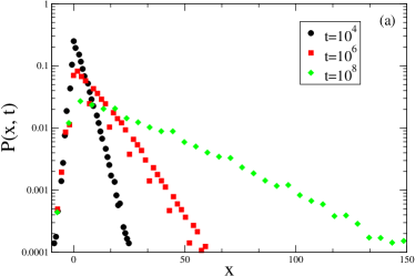
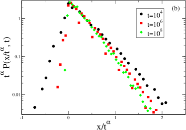
Figure 1: Probability distribution of displacements $P_{\epsilon}(x,t)$ for an asymmetric CTRW (at each step the probability to move left or right is respectively $p_{l}=(1-\epsilon)/2$ and $p_{r}=(1+\epsilon)/2$, with $\epsilon=0.3$) with exponent $\alpha=1/4$ of waiting time distribution $p(\tau)=\tau^{-(1+\alpha)}$. Left: $P_{\epsilon}(x,t)$ at $t=10^{4},10^{6},10^{8}$ in semilog scale; Right: $P_{\epsilon}(x,t)$ at $t=10^{4},10^{6},10^{8}$ in semilog scale with data collapsed according to the scaling form $P_{\epsilon}(x,t)=t^{-\alpha}F_{\epsilon}(x/t^{\alpha})$.

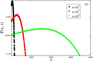
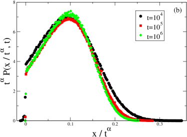
Figure 2: Probability distribution of displacements $P_{\epsilon}(x,t)$ for an asymmetric CTRW (at each step the probability to move left or right is respectively $p_{l}=(1-\epsilon)/2$ and $p_{r}=(1+\epsilon)/2$, with $\epsilon=0.3$) with exponent $\alpha=3/4$ of waiting time distribution $p(\tau)=\tau^{-(1+\alpha)}$. Left: $P_{\epsilon}(x,t)$ at $t=10^{4},10^{5},10^{6}$ in semilog scale; Right: $P_{\epsilon}(x,t)$ at $t=10^{4},10^{5},10^{6}$ in linear scale with data collapsed according to the scaling form $P_{\epsilon}(x,t)=t^{-\alpha}F_{\epsilon}(x/t^{\alpha})$.

III.3 Numerical results for the probability distribution: $1/2<\alpha<1$

The scaling picture for $1/2<\alpha<1$ is analogous to the case with $\alpha<1/2$, and the scaling length of the process is $\ell(t)\sim t^{\alpha}$. In this situation we observe the onset of a field-induced superdiffusive spreading of $P_{\epsilon}(x,t)$ in a regime where in absence of an external field the behavior is still subdiffusive, $\langle x(t)^{2}\rangle_{0}\sim t^{\alpha}$. The main difference with respect to the previous case is that now the peak of the distribution moves as $x_{p}(t)\sim t^{\alpha}\sim\ell(t)$ and the scaling form reads:

$$P(x,t)\sim\frac{1}{t^{\alpha}}F\left(\frac{\xi}{t^{\alpha}}\right)\sim\frac{1}{t^{\alpha}}F\left(\frac{|x-v_{sub}t^{\alpha}|}{t^{\alpha}}\right)\sim\frac{1}{t^{\alpha}}G\left(\frac{x}{t^{\alpha}}\right)$$ (14)

where $\alpha>1/2$. Fig. 2 shows that the scaling assumption in Eq. (14) is well verified. Interestingly, as clearly seen from Fig.s 1 and 2, while before the rescaling the behavior of the probability distribution at $1/2<\alpha<1$ looks very different from that observed in the case $\alpha<1/2$, after rescaling the two curves display the same behavior and the only difference is the position of the peak at $x=0$ and at $x>0$. Also in this regime, we observe a weak anomalous diffusion, because there is a single scaling length in the problem, $\ell(t)=t^{\alpha}$, and all the higher order cumulants can be written as functions of this scaling length: $\langle\left[\delta x(t)\right]^{n}\rangle_{\epsilon}\sim\ell^{n}(t)$.

III.4 Numerical results for the probability distribution: $1<\alpha<2$

For $1<\alpha<2$ the drift of the distribution $P_{\epsilon}(x,t)$ becomes linear, $x_{p}(t)\sim\langle x(t)\rangle_{\epsilon}\sim t$, and now the probability of finding a particle at a distance $\xi=x-x_{p}(t)$ from the peak of the distribution at time $t$ can be evaluated with a simple scaling argument. In particular the probability of remaining at a distance $\xi$ from $x_{p}(t)$ is due to the probability for a walker to experience a stop of duration $\tau\sim\xi$. For each scattering event the probability of waiting a time $\tau\sim\xi$ is then

$$p_{\alpha}(\tau)d\tau=p_{\alpha}(\tau(\xi))\frac{d\tau}{d\xi}d\xi\sim\frac{1}{\xi^{1+\alpha}}d\xi,$$ (15)

Since the number of steps $N(t)$ in a time $t$ is also proportional to $t$, the tail of the distribution at large $\xi$ can be estimated as:

$$P_{\epsilon}(\xi,t)\sim\frac{N(t)}{\xi^{1+\alpha}}\sim\frac{t}{\xi^{1+\alpha}},$$ (16)

which corresponds to a scaling form:

$$P_{\epsilon}(\xi,t)=\frac{1}{t^{1/\alpha}}F\left(\frac{\xi}{t^{1/\alpha}}\right)=\frac{1}{t^{1/\alpha}}F\left(\frac{|x-vt|}{t^{1/\alpha}}\right).$$ (17)

Introducing the cut-off in zero to calculate the higher order cumulants of the $P_{\epsilon}(x,t)$, we obtain

$$\langle\left[\delta x(t)\right]^{n}\rangle_{\epsilon}=\frac{1}{t^{1/\alpha}}\int_{0}^{t}d\xi~{}\xi^{n}~{}F\left(\frac{\xi}{t^{1/\alpha}}\right)\sim t\int_{0}^{t}d\xi~{}\xi^{n-1-\alpha}\sim t^{n+1-\alpha}.$$ (18)

In the case of $1<\alpha<2$ the effect of a fat tail connecting the center of the distribution to the origin is to produce a strong anomalous diffusion, because the scaling length of the distribution is $\ell(t)\sim t^{\alpha/2}$ and from Eq. (18) we see that $\langle\left[\delta x(t)\right]^{n}\rangle_{\epsilon}\neq\ell^{n}(t)$.

Detailed analytical computations are reported in noi and are in very good agreement with the results of numerical simulations, as shown in Fig. 3 for $\alpha=1.5$.

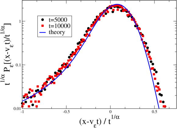
Figure 3: Probability distributions $P_{\epsilon}(x,t)$ of the Continuous Time Random Walk with trapping, calculated at different times in numerical simulations, are collapsed here according to the scaling form in Eq. (17), with exponent $\alpha=3/2$ and $v_{\epsilon}=0.1$. Symbols correspond to different times, as shown in the legend. The continuous line represents the analytical result reported in noi .

IV Rare events and scaling in the Lévy Walk

IV.1 Scaling from the matching argument

In the Lévy walk model the probe particle performs free flights with velocities $v_{i}$ extracted from a Gaussian distribution, and of duration $\tau_{i}$, with a total displacement which is, in absence of the field, $x(t)=\sum_{i}^{N(t)}\tau_{i}v_{i}$, where $N(t)$ is the number of steps up to the elapsed time $t$. In this model the external field $\epsilon$ acts as a constant acceleration, so that the total displacement in a trajectory becomes $x(t)=\sum_{i}^{N(t)}\tau_{i}v_{i}+\epsilon\tau_{i}^{2}$. The mean value and the second moment of $x(t)$ can be evaluated analogously to the CTRW with trapping as:

$$\langle x(t)\rangle_{\epsilon}=\left\langle\sum_{i=1}^{N(t)}x_{i}\right\rangle_{\epsilon}=\overline{N(t)}\langle\tau_{i}^{2}\rangle_{\epsilon},$$ (19)

and

$$\langle x^{2}(t)\rangle_{\epsilon}-\langle x(t)\rangle_{\epsilon}^{2}=\overline{N(t)}\left(\langle v_{i}^{2}\rangle+\epsilon^{2}(\langle\tau_{i}^{4}\rangle_{c}-\langle\tau_{i}^{2}\rangle_{c}^{2})\right)+\left(\overline{N(t)^{2}}+\Delta(N)^{2}\right)\epsilon^{2}\langle\tau_{i}\rangle^{2}_{c},$$ (20)

where we used the fact that $\langle v_{i}\rangle=0$. Moreover, in order to avoid divergences, we introduce the same cutoff $t_{c}$ in the evaluation of the average of the flights time and of its moments, using for this purpose again the modified distribution (10). Also in this case the average number of steps in a time $t$ and its variance can be evaluated as $N(t)=t/\langle\tau\rangle_{c}$ and $\Delta(N)^{2}=t\Delta_{c}(\tau)^{2}/\langle\tau\rangle_{c}^{3}$. Finally, the divergences can be taken safely into account letting the cutoff $t_{c}\rightarrow t$ i.e. the maximum time of flight allowed in a time $t$  ACMV00 .

In the case $\alpha>4$ all the expectation values in Eqs. (19,20) are finite and one recovers the standard formulas for diffusion with drift i.e. $\langle x(t)\rangle_{\epsilon}\sim t$ and $\langle x^{2}(t)\rangle_{\epsilon}-\langle x(t)\rangle_{\epsilon}^{2}\sim t$. For $2<\alpha<4$ we get a standard behavior for the drift $\langle x(t)\rangle_{\epsilon}\sim t\epsilon$. However, in the evaluation of the variance we have to take into account that $\langle\tau_{i}^{4}\rangle$ is diverging and, setting the cut of at $t_{c}=t$, we have $\langle x^{2}(t)\rangle_{\epsilon}-\langle x(t)\rangle_{\epsilon}^{2}\sim t^{5-\alpha}\epsilon^{2}$. Therefore, the system features a strong anomalous behavior in a regime where in absence of forcing a normal diffusion is observed. In the regime $1<\alpha<2$, the variance has the same behavior but an anomalous drift $\langle x(t)\rangle_{\epsilon}\sim t^{3-\alpha}$ is present, since $\langle\tau_{i}\rangle$ diverges as $t^{2-\alpha}$. Finally for $\alpha<1$ the motion is accelerated $\langle x(t)\rangle_{\epsilon}\sim t^{2}$ and $\langle x^{2}(t)\rangle_{\epsilon}-\langle x(t)\rangle_{\epsilon}^{2}\sim t^{4}$.

IV.2 Scaling from the single long jump hypothesis

The matching argument allows us to evaluate the behavior of the first and second moment of the distribution $P_{\epsilon}(x,t)$; we now introduce another simple argument for estimating the scaling properties of $P_{\epsilon}(x,t)$ assuming that the behaviour of higher order moments/cumulants is due to a fat (right) tail and that the behaviour of the tail is generated by isolated rare events  Levyrandom . This means that the probability of finding a particle at a very large distance $\xi$ from $x_{p}(t)$, the peak of the distribution, is given by the probability that this particle has reached $\xi$ thanks to a single long jump Levyrandom . Therefore, due to the constant acceleration of the particle, the large distribution of displacements in single jumps is related to the large distribution of flight times through the change of variables $\xi=v\tau+\epsilon/2\tau^{2}$, which for large time can be approximated as $\xi\sim\tau^{2}$. From this we can obtain the distribution of displacements in a single jump in presence of the field:

$$p(\tau)d\tau=p(\tau(\xi))\frac{d\tau}{d\xi}d\xi\sim\frac{1}{\xi^{1+\alpha/2}}d\xi.$$ (21)

From this relation, we can predict that the general scaling form of the fat tail of $P_{\epsilon}(x,t)$ will be related to trajectories dominated by a single long jump $\xi$, performed in one of the steps $N(t)$. We have:

$$P_{\epsilon}(x,t)\sim\frac{N(t)}{(x-x_{p}(t))^{1+\alpha/2}}.$$ (22)

Let us now consider separately the different regimes for the scaling form of the probability distribution.

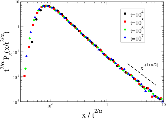
Figure 4: Probability distribution of displacements $P_{\epsilon}(x,t)$ for the Levy walk with exponent $\alpha=1/2$ of free fights time distribution $p(\tau)=\tau^{-(1+\alpha)}$. The three curves (log-log scale) represent data at times $t=10^{4},10^{5},10^{6}$, collapsed according to the scaling form $P_{\epsilon}(x,t)=t^{-2}F_{\epsilon}(x/t^{2})$.

IV.3 Numerical results for the probability distribution: $\alpha<1$

In this regime, strong anomalous diffusion is not present and an accelerated growth of the scaling length $\ell(t)\sim t^{2}$ determines the whole dynamics. In particular also the peak of the distribution grows as $x_{p}(t)\sim t^{2}$ and the scaling form in Eq. (22) becomes

$$P_{\epsilon}(x,t)=\frac{1}{t^{2}}F\left(\frac{x-x_{p}(t)}{t^{2}}\right)=\frac{1}{t^{2}}G\left(\frac{x}{t^{2}}\right),$$ (23)

This can be clearly seen in Fig.4 at $\alpha=1/2$. The scaling form predicted is in excellent agreement with the simulations. We remark that since the scaling length is of order $t^{2}$, it is not possible that a single long jump of order $t^{2}$ dominates the transport process.

IV.4 Numerical results for the probability distribution: $1<\alpha<2$

Numerical simulations show that the peak of the distribution moves as $x_{p}(t)=t^{2/\alpha}$ In this case the asymptotic behavior at large $\xi$ described in Eq. (22) is satisfied by the probability distribution and can be used to infer its scaling properties:

$$P_{\epsilon}(x,t)=\frac{t}{\xi^{1+\alpha/2}}=\frac{1}{t^{2/\alpha}}F\left(\frac{x-x_{p}(t)}{t^{2/\alpha}}\right)=\frac{1}{t^{2/\alpha}}G\left(\frac{x}{t^{2/\alpha}}\right),$$ (24)

with $F(y)=y^{-(1+\alpha/2)}$. Here we used the fact that in this regime $N(t)\sim t$ and that $x_{p}(t)$ grows as $t^{2/\alpha}$ in order to define the new scaling function $G(\cdot)$.

The distribution computed in numerical simulations is shown in Fig. 5 for $\alpha=1.5$ featuring a nice data collapse.

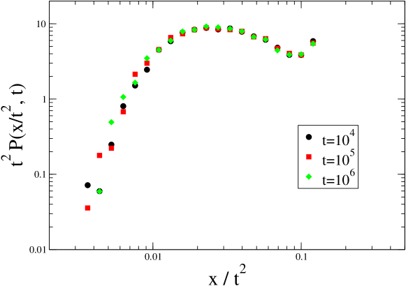
Figure 5: Probability distribution of displacements $P_{\epsilon}(x,t)$ for the Levy walk model with bias (log-log scale).times is obtained with the scaling form in Eq.(24), with exponent $\alpha=3/2$. Symbols correspond to different times, as shown in the legend. In figure is highlighted the power law behaviour $F(y)\sim y^{-(1+\alpha/2)}$ (dashed line) of the scaling function $F(y)$ (see text).

IV.5 Numerical results for the probability distribution: $2<\alpha<4$

In this case the peak of the distribution moves linearly $x_{p}(t)\sim t$ and the scaling form in Eq. (22) becomes

$$P_{\epsilon}(\xi,t)=\frac{t}{\xi^{1+\alpha/2}}=\frac{1}{t^{2/\alpha}}F\left(\frac{\xi}{t^{2/\alpha}}\right)=\frac{1}{t^{2/\alpha}}F\left(\frac{x-vt}{t^{2/\alpha}}\right),$$ (25)

with $F(y)=y^{-(1+\alpha/2)}$.

In the case of the Lévy walk the superdiffusion is strong anomalous for all values of the exponent $\alpha$ as we always have $\langle\left[\delta x(t)\right]^{n}\rangle_{\epsilon}\neq\ell^{n}(t)$.

Detailed analytical computations are reported in noi and are in very good agreement with the results of numerical simulations, as shown in Fig. 6 for $\alpha=2.5$.

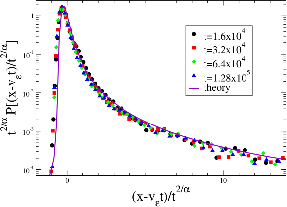
Figure 6: Probability distribution of displacements $P_{\epsilon}(x,t)$ for the Levy walk model with bias (semi-log scale).The collapse of curves at different times is obtained with the scaling form in Eq.(25), with exponent $\alpha=5/2$. Symbols correspond to different times, as shown in the legend. The line represents the analytical results for the distribution reported in noi .

V Conclusion

We have studied the scaling properties of the displacement probability distribution functions for a CTRW with trapping and for the Lévy walk in an arbitrary small field and we have shown that the presence of the field introduces new length-scales related to rare events. Beyond the principal scaling length of the distribution $\ell(t)$ and that related to the rigid shift, $\ell_{T}(t)$, one must also consider the typical length introduced by the cut-off of the power-law tail, $\ell_{e}(t)$, necessary for the calculation of higher order moments. This is how rare events induce the strong anomalous behavior.

The scaling properties of probability distribution function and of all its moments can be obtained by estimating the effect of the additional length scales on the process. This has been done by two heuristic yet powerful techniques, the matching condition and the single long jump hypothesis, with excellent agreement with the analytical results obtained from the master equations, and also in excellent agreement with extensive numerical simulations. These heuristic approaches are flexible and could be useful to analyze models where one is not able to solve the master equations for the process in the asymptotic region.

The change in transport properties in the presence of an external field represents an interesting probe to investigate the microscopic dynamical features of the system. Field-induced anomalous behavior highlights the importance of rare and large fluctuations in regimes where the diffusion properties are apparently standard.

References

References

- (1) F. Bardou, J.-P. Bouchaud, A. Aspect, and C. Cohen-Tannoudji, 2001 Lévy Statistics and Laser Cooling: How Rare Events Bring Atoms to Rest (Cambridge University Press, Cambridge).
- (2) B. Wang, J. Kuo, S. C. Bae, and S. Granick, 2012 Nature Materials 485 11 .
- (3) L. H. Tang and H. Chaté, 2001 Phys. Rev. Lett. 86 830.
- (4) A. D. Sánchez, J. M. López, M. A. Rodríguez, and M. A. Matías, 2004 Phys. Rev. Lett. 92 204101.
- (5) J.-P. Bouchaud and A. Georges, 1990 Phys. Rep. 195 127.
- (6) P. Ribière, P. Richard, R. Delannay, D. Bideau, M. Toiya, and W. Losert, 2005 Phys. Rev. Lett. 95 268001.
- (7) R. Burioni, G. Gradenigo, A. Sarracino, A. Vezzani, and A. Vulpiani, 2013 J. Mech. Stat. P09022.
- (8) O. Bénichou, C. Mejía-Monasterio, and G. Oshanin, 2013 Phys. Rev. E 87 020103(R).
- (9) O. Bénichou, P. Illien, C. Mejía-Monasterio, and G. Oshanin, 2013 J. Stat. Mech. P05008.
- (10) E. Barkai and V. Fleurov, 1998 Phys. Rev. E 58 1296.
- (11) S. Jespersen, R. Metzler, and H. C. Fogedby, 1999 Phys. Rev. E 59 2736.
- (12) D. Villamaina, A. Sarracino, G. Gradenigo, A. Puglisi and A. Vulpiani, 2011 J. Stat. Mech. L01002.
- (13) U. Marini Bettolo Marconi, A. Puglisi, L. Rondoni, and A. Vulpiani, 2008 Phys. Rep. 461 111.
- (14) O. Bénichou, P. Illien, G. Oshanin, and R. Voituriez, 2013 Phys. Rev. E 87 032164.
- (15) D. Winter, J. Horbach, P. Virnau and K. Binder, 2012 Phys. Rev. Lett.108 028303.
- (16) C. F. E. Schroer and A. Heuer, 2013 Phys. Rev. Lett. 110 067801.
- (17) O. Bénichou, A. Bodrova, D. Chakraborty, P. Illien, A. Law, C. Mejía-Monasterio, G. Oshanin, and R. Voituriez, 2013 Phys. Rev. Lett. 111 260601.
- (18) P. Castiglione, A. Mazzino, P. Muratore-Ginanneschi, and A. Vulpiani, 1999 Physica D 134 75.
- (19) K. H. Andersen, P. Castiglione, A. Mazzino, and A. Vulpiani, 2000 Eur. Phys. J. B 18 447.
- (20) R. Burioni, L. Caniparoli, and A. Vezzani, 2010 Phys. Rev. E 81 060101.
- (21) L. Angelani, R. Di Leonardo, G. Parisi, and G. Ruocco, 2001 Phys. Rev. Lett. 87 055502.
- (22) P. Levitz, 1997 Europhys. Lett. 39 593.
- (23) D. ben-Avraham and S. Havlin, 2004 Diffusion and Reactions in Fractals and Disordered Systems (Cambridge University Press (Cambridge University Press).
- (24) P. Buonsante, R. Burioni and A. Vezzani, 2011 Phys. Rev. E 84 021105.
- (25) R. Burioni, E. Ubaldi, A. Vezzani, 2014 Phys. Rev. E 89 022135.
- (26) C. W. Groth, A. R. Akhmerov, and C. W. J. Beenakker, 2012 Phys. Rev. E 85 021138.
- (27) O. Bénichou, C. Loverdo, M. Moreau, and R. Voituriez, 2011 Rev. Mod. Phys. 83 81.
- (28) M. F. Shlesinger and J. Klafter, 1985 Phys. Rev. Lett. 54 2551.
- (29) F. Lechenault, R. Candelier, O. Dauchot, J.-P. Bouchaud and G. Biroli, 2012 Soft Matter 6 3059.
- (30) P. Barthelemy, J. Bertolotti and D. S. Wiersma, 2008 Nature 453 495.
- (31) R. Klages, G. Radons and I. M. Sokolov (Eds.), 2008 Anomalous Transport: Foundations and Applications (Wiley, VCH Berlin).
- (32) I. M. Sokolov and R. Metzler, 2003 Phys. Rev. E 67 010101(R).
- (33) G. Gradenigo, A. Sarracino, D. Villamaina, and A. Vulpiani, 2012 J. Stat. Mech. L06001.