Detection of weak forces based on noise-activated switching in bistable optomechanical systems

Abstract

We propose to use cavity optomechanical systems in the regime of optical bistability for the detection of weak harmonic forces. Due to the optomechanical coupling an external force on the mechanical oscillator modulates the resonance frequency of the cavity and consequently the switching rates between the two bistable branches. A large difference in the cavity output fields then leads to a strongly amplified homodyne signal. We determine the switching rates as a function of the cavity detuning from extensive numerical simulations of the stochastic master equation as appropriate for continuous homodyne detection. We develop a two-state rate equation model that quantitatively describes the slow switching dynamics. This model is solved analytically in the presence of a weak harmonic force to obtain approximate expressions for the power gain and signal-to-noise ratio that we then compare to force detection with an optomechanical system in the linear regime.

I Introduction

The field of cavity optomechanics is historically closely related to the problem of force sensing in the context of gravitational wave detection Braginsky (1968); Braginsky and Vorontsov (1975); Caves (1980); Caves et al. (1980), and the fundamental limit of force sensitivity can be traced back to the quantum-mechanical nature of the detector, the so-called standard quantum limit Braginsky and Khalili (1992).

Most optomechanical devices to date operate in the regime where the radiation pressure is sufficiently weak on the single-photon level so the coupling between phonons and photons can be linearized. Examples for exciting progress in this area include the observation of ground-state cooling Teufel et al. (2011); Rivière et al. (2011); Chan et al. (2011), ponderomotive squeezing Brooks et al. (2012); Safavi-Naeini et al. (2013); Purdy et al. (2013a), radiation-pressure shot-noise Murch et al. (2008); Purdy et al. (2013b), and mechanical zero-point motion via sideband thermometry Safavi-Naeini et al. (2012); Brahms et al. (2012); Lee et al. (2014); Purdy et al. (2014) as well as the demonstration of displacement detection close to the standard quantum limit Anetsberger et al. (2009); Schliesser et al. (2009); Teufel et al. (2009); Schreppler et al. (2014).

Advances in fabricating optomechanical devices promise increasingly large coupling strengths Chan et al. (2012) making nonlinear quantum effects Nunnenkamp et al. (2011); Rabl (2011) a possible reality in the near future. It is thus of great interest to study how the intrinsically nonlinear radiation pressure can be exploited in novel devices.

In this paper we propose sensitive force detection exploiting optical bistability in an optomechanical system Dorsel et al. (1983); Meystre et al. (1985); Aldana et al. (2013). The optomechanical system we consider consists of a laser-driven optical cavity whose resonance frequency is modulated by the displacement of a mechanical oscillator Kippenberg and Vahala (2008); Marquardt and Girvin (2009); Aspelmeyer et al. (2013). Under certain conditions the system exhibits an optical bistability, i.e. it has two classically stable states with potentially largely different cavity fields. Shot-noise fluctuations in the coherent drive of the cavity will cause transitions between the two branches whose switching rates can depend strongly on cavity detuning. A weak periodic forcing of the mechanical resonator will modulate the cavity detuning and thus the switching rates allowing the detection of weak forces in the cavity spectrum.

Note that exploiting periodic modulation of switching rates in bistable systems to detect small coherent signals has also been discussed in the context of stochastic resonance Gammaitoni et al. (1998); Wellens et al. (2004); Venstra et al. (2013) and Josephson bifurcation amplifiers Manucharyan et al. (2007); Mallet et al. (2009); Vijay et al. (2009).

In the following we calculate numerically the switching dynamics in the single-photon strong-coupling regime and zero temperature limit using a stochastic quantum master equation. We obtain the switching rates and their dependence on the detuning from the residence time distribution. We then develop a two-state rate equation model allowing us to write the output spectral density of the amplitude quadrature as the sum of a low-frequency noise background and a signal peak caused by the weak harmonic force. The homodyne signal amplitude depends linearly on the force amplitude and on the difference between the cavity output fields. Bistable optomechanical systems can thus be used as linear amplifiers whose bandwidth is the switching rate and which have a potentially large gain for low-frequency signals.

The remainder of the present paper is organized as follows. In Sec. II we introduce the model for an optomechanical system (OMS) with an additional external force driving the mechanical oscillator and present the stochastic master equation describing the system state conditioned on continuous homodyne detection. In Sec. III we investigate numerically noise-induced switching in a bistable OMS. We obtain time traces of the homodyne photocurrent, the residence time distributions, and the switching rates as a function of cavity detuning. In Sec. IV we describe the slow switching dynamics and the influence of a harmonic force within a two-state rate equation model with periodically modulated switching rates. In Sec. V we find expressions for the noise spectral density and the signal amplitude of the homodyne photocurrent, based on the two-state rate equation model, and compare them to quantum trajectory results. Finally, we compare the power gain and signal-to-noise ratio of force detection with a bistable OMS to those achievable with an OMS in the linear regime.

II Model

We consider an optomechanical system (OMS) in which the position of a mechanical oscillator modulates the resonance frequency of an optical cavity. The system consists of a mechanical mode with resonance frequency $\omega_{m}$ and an optical mode with frequency $\omega_{c}$ which are coupled by the radiation-pressure interaction. The optical mode is driven by a laser with strength $\epsilon$ and frequency $\omega_{d}$. In a frame rotating at the drive frequency $\omega_{d}$ the Hamiltonian reads $(\hbar=1)$

$$\hat{H}=-\Delta_{0}\hat{a}^{\dagger}\hat{a}-i\epsilon\left(\hat{a}-\hat{a}^{\dagger}\right)+\omega_{m}\hat{b}^{\dagger}\hat{b}-g_{0}\hat{a}^{\dagger}\hat{a}\left(\hat{b}+\hat{b}^{\dagger}\right)\>,$$ (1)

where $\hat{a}$ and $\hat{b}$ are bosonic annihilation operators for the optical and mechanical mode, $\Delta_{0}=\omega_{d}-\omega_{c}$ is the detuning between driving and cavity frequency, and $g_{0}$ is the optomechanical coupling. We also add an external periodic force on the mechanical resonator with amplitude $g_{1}$ and frequency $\Omega$

$$\hat{H}_{F}=-g_{1}\sin(\Omega t)\left(\hat{b}+\hat{b}^{\dagger}\right)\>.$$ (2)

A complete description of the system additionally requires the optical damping rate $\kappa$, the mechanical energy dissipation rate $\gamma_{m}$, and the mean phonon number in thermal equilibrium $n_{\text{th}}=0$ corresponding to a zero-temperature reservoir.

The dissipative dynamics of the OMS undergoing continuous homodyne measurement of the cavity output can be described with the Itô stochastic master equation (SME) Wiseman and Milburn (1993, 2009)

$$d\hat{\rho}_{c}=\mathcal{L}[\hat{\rho}_{c}]dt+\mathcal{H}[\hat{\rho}_{c}]dW\>,$$ (3)

$$\mathcal{L}[\hat{\rho}_{c}]=-i\left[\hat{H}+\hat{H}_{F},\hat{\rho}_{c}\right]+\kappa\mathcal{D}_{\hat{a}}[\hat{\rho}_{c}]$$

$$\qquad\qquad+\left(n_{\text{th}}+1\right)\gamma_{m}\mathcal{D}_{\hat{b}}[\hat{\rho}_{c}]+n_{\text{th}}\gamma_{m}\mathcal{D}_{\hat{b}^{\dagger}}[\hat{\rho}_{c}]\>,$$ (4)

$$\mathcal{H}[\hat{\rho}_{c}]=\sqrt{\kappa}\left(\hat{a}\hat{\rho}_{c}+\hat{\rho}_{c}\hat{a}^{\dagger}-\left\langle\hat{a}+\hat{a}^{\dagger}\right\rangle_{c}\hat{\rho}_{c}\right)\>,$$ (5)

where $d\rho_{c}=\hat{\rho}_{c}(t+dt)-\hat{\rho}_{c}(t)$, $\langle\hat{a}+\hat{a}^{\dagger}\rangle_{c}=\text{Tr}[(\hat{a}+\hat{a}^{\dagger})\hat{\rho}_{c}]$, and $dW$ is a Wiener increment with $\text{E}[dW]=0$ and $\text{E}[dW^{2}]=dt$. $\text{E}[-]$ is the ensemble average and the Lindblad terms have the usual form, $\mathcal{D}_{\hat{o}}[\hat{\rho}]=\hat{o}\hat{\rho}\hat{o}^{\dagger}-(\hat{o}^{\dagger}\hat{o}\hat{\rho}+\hat{\rho}\hat{o}^{\dagger}\hat{o})/2$. The first term in Eq. (3) is the Liouvillian describing the coherent evolution due to the Hamiltonian and the decoherence originating from the coupling to the environment. The second term called innovation describes the effect of a measurement of the amplitude quadrature, $\hat{X}=\hat{a}+\hat{a}^{\dagger}$, with homodyne detection of the cavity output field. The innovation term conditions the evolution of the quantum state $\hat{\rho}_{c}(t)$ on the homodyne photocurrent

$$I_{c}(t)=\sqrt{\kappa}\big{\langle}\hat{X}(t)\big{\rangle}_{c}+\frac{dW}{dt}\>,$$ (6)

which is the sum of a conditioned expectation value of $\hat{X}$ and a fluctuating term originating from the shot noise of the local oscillator (here we have assumed unit detection efficiency).

We will refer to the result for a particular noise realization of $\hat{\rho}_{c}(t)$ and $I_{c}(t)$ as a quantum trajectory. Taking the ensemble average of Eq. (3) we recover the unconditional quantum state $\hat{\rho}(t)=\text{E}[\hat{\rho}_{c}(t)]$ which is a solution to the quantum master equation

$$\dot{\hat{\rho}}=\mathcal{L}[\hat{\rho}]\>.$$ (7)

In the following we calculate the evolution of the quantum state $\hat{\rho}_{c}(t)$ by numerically integrating Eq. (3) Kloeden and Platen (1992) and use the time traces of the homodyne photocurrent $I_{c}(t)$ to investigate the switching dynamics in the regime of optical bistability.

To quantify the influence of the external mechanical force on the cavity output we use the time-averaged spectral density

$$S_{II}^{\text{out}}(\omega)=\lim_{t\to\infty}\int d\tau\,e^{i\omega\tau}\text{E}\left[I_{c}(t+\tau)I_{c}(t)\right]\>.$$ (8)

For finite, but sufficiently long sampling times $T$ the spectral density can be obtained using the Wiener-Khintschin theorem from a quantum trajectory as $S_{II}^{\text{out}}(\omega)=|I_{T}(\omega)|^{2}$ where

$$I_{T}(\omega)=\frac{1}{\sqrt{T}}\int_{0}^{T}dt\,e^{i\omega t}I_{c}(t)$$ (9)

is the windowed Fourier transform of the homodyne photocurrent $I_{c}(t)$. In this way we replace the ensemble average by a time average. In the following we will numerically simulate a single, sufficiently long quantum trajectory instead of calculating averages over an ensemble of quantum trajectories.

III Noise-activated switching in bistable OMS

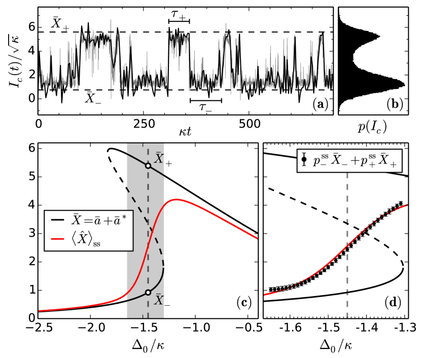
Figure 1: (Color online) Noise-activated switching in a bistable optomechanical system (OMS). (a) Homodyne photocurrent $I_{c}(t)$ for a representative quantum trajectory. The OMS switches between two bistable states that are close to the two stable solutions $\bar{X}_{\pm}$ (dashed lines) of the nonlinear mean-field equations (MFEs) (10). From the time trace $I_{c}(t)$ the residence times $\tau_{\pm}$ can be extracted. We show both the conditioned expectation value of the amplitude quadrature $\langle\hat{X}(t)\rangle_{c}$ (grey solid) and the homodyne photocurrent $I_{c}(t)$ after applying a low-pass filter (black solid). (b) From a sufficiently long trajectory we can obtain the probability distribution $p(I_{c})$ of the filtered homodyne photocurrent whose double-peak structure is a signature of the bistable behavior. (c) Stable $\bar{X}_{\pm}$ (black solid) and unstable (black dashed) solutions to the MFEs (10) as a function of the bare detuning $\Delta_{0}$. We indicate the stable states (circles) between which the system shown in (a) and (b) switches. The figure also shows the steady-state expectation value $\langle\hat{X}\rangle_{\text{ss}}$ (red solid) interpolating between the bistable solutions $\bar{X}_{\pm}$. (d) A blow-up of the region marked grey in panel (c). Additionally, we plot the weighted average of the mean-field solutions $p_{-}^{\text{ss}}\bar{X}_{-}+p_{+}^{\text{ss}}\bar{X}_{+}$ (black dots) where the probabilities $p_{\pm}^{\text{ss}}$ are given by Eq. (11). The parameters are $\omega_{m}/\kappa=5$, $\gamma_{m}/\kappa=1/2$, $g_{0}/\kappa=1/\sqrt{2}$, $\epsilon/\kappa=1.5$, and $\Delta_{0}/\kappa=-1.45$ (a,b).

We investigate the dynamics of an OMS in a regime where the mechanical resonator acts like an effective Kerr nonlinearity for the optical mode Aldana et al. (2013). As a consequence the system can exhibit optical bistability, a phenomenon characterized by the presence of two stable mean-field states. In a semiclassical approximation the steady-state amplitudes of the optical $\bar{a}$ and mechanical modes $\bar{b}$ are obtained by solving the coupled mean-field equations (MFEs)

$$0 =\left(i\Delta_{0}-\frac{\kappa}{2}\right)\bar{a}+ig_{0}\bar{a}\left(\bar{b}+\bar{b}^{*}\right)+\epsilon,$$ (10)

$$0 =-\left(i\omega_{m}+\frac{\gamma_{m}}{2}\right)\bar{b}+ig_{0}|\bar{a}|^{2}\>.$$

An analysis of the nonlinear MFEs (10) shows that the OMS undergoes a bifurcation when the driving amplitude exceeds the threshold value $\epsilon_{\text{bif}}=3^{1/4}(\kappa^{3}\omega_{m}/18)^{1/2}/g_{0}$. As a consequence three solutions for $\bar{a}$ exist in a certain range of negative detuning $\Delta_{0}$. The two solutions $\bar{a}_{\pm}$ with the smallest and largest amplitude $|\bar{a}|$ are stable and referred to as the upper and lower branches of the bistable system.

Shot-noise fluctuations in the cavity drive will cause transitions between the stable branches. This effect dubbed noise-activated switching has been investigated e.g. in the case of a Kerr medium theoretically Rigo et al. (1997); Dykman et al. (2005); Dykman (2007, 2012); Peano and Dykman (2014) and experimentally Kerckhoff et al. (2011).

In Fig. 1(a) we show the homodyne photocurrent $I_{c}(t)$ for a representative quantum trajectory. We observe that the OMS switches between two bistable states characterized by two different values of $I_{c}(t)$ and corresponding approximately to $\sqrt{\kappa}\bar{X}_{\pm}$ where $\bar{X}_{\pm}=\bar{a}_{\pm}+\bar{a}_{\pm}^{*}$. After applying a low-pass filter to the raw quantum trajectory data we can extract the residence times $\tau_{\pm}$ from the time trace $I_{c}(t)$. From a sufficiently long trajectory we obtain the probability distribution $p(I_{c})$ for the homodyne photocurrent, shown in Fig. 1(b). It features a double peak, a signature of the bistable behavior.

In Fig. 1(c) we show the mean-field amplitude quadrature, $\bar{X}=\bar{a}+\bar{a}^{*}$, as function of the detuning $\Delta_{0}$ obtained from the solutions to the nonlinear MFEs (10). We also calculate the steady-state expectation value $\langle\hat{X}\rangle_{\text{ss}}$ from the QME (7) which interpolates between the two bistable solutions $\bar{X}_{\pm}$.

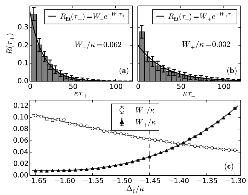
Figure 2: (Color online) Residence time distributions and switching rates. (a) Histogram $R(\tau_{+})$ of residence times in the upper branch extracted from the quantum trajectory in Fig. 1(a) with statistical error bars. The solid line is an exponential fit $R_{\text{fit}}(\tau_{+})=W_{-}e^{-W_{-}\tau_{+}}$ excluding the first bin. (b) Same as (a) but for the residence times in the lower branch. We determine the switching rate $W_{+}$ by fitting the histogram $R(\tau_{-})$ with the distribution $R_{\text{fit}}(\tau_{-})=W_{+}e^{-W_{+}\tau_{-}}$ . (c) Switching rates $W_{\pm}$ as a function of $\Delta_{0}$. Parameters are identical to those in Fig. 1 and with $\Delta_{0}/\kappa=-1.45$ (a,b).

Figures 2(a) and 2(b) show histograms $R(\tau_{\pm})$ of residence times in the upper and lower branches, respectively, which we extracted from the quantum trajectory shown in Fig. 1(a) including statistical error bars. We fit the data with exponential distribution functions $R_{\text{fit}}(\tau_{\pm})=W_{\mp}\exp(-W_{\mp}\tau_{\pm})$ and determine the switching rates $W_{\mp}$ from the upper to the lower branch and vice versa . In Fig. 2(c) we plot the switching rates $W_{\pm}$ as a function of cavity detuning $\Delta_{0}$.

In steady state the probability to find the OMS in the upper or lower branch, $p_{\pm}^{\text{ss}}$, is related to the switching rates via

$$p_{\pm}^{\text{ss}}=\frac{W_{\pm}}{W_{+}+W_{-}}\>.$$ (11)

The probability $p_{\pm}^{\text{ss}}$ is the fraction of time spent by the system in the upper and lower branch, respectively. It can be written as $T_{\pm}/(T_{+}+T_{-})$, where $T_{\pm}$ is the average residence time and is given by $T_{\pm}=\int\tau_{\pm}R(\tau_{\pm})d\tau_{\pm}=W_{\mp}^{-1}$.

If the fluctuations in each branch $\bar{a}_{\pm}$ are small compared to their phase-space separation $|\bar{a}_{+}-\bar{a}_{-}|$, the average homodyne photocurrent $I_{\text{ss}}=\text{E}[I_{c}(t)]$, or equivalently the steady-state expectation value $\langle\hat{X}\rangle_{\text{ss}}=I_{\text{ss}}/\sqrt{\kappa}$, is well approximated by the weighted average of the mean-field solutions

$$I_{\text{ss}}\simeq\sqrt{\kappa}\left(p_{-}^{\text{ss}}\bar{X}_{-}+p_{+}^{\text{ss}}\bar{X}_{+}\right)\>.$$ (12)

In Fig. 1(d) we show a blow up of Fig. 1(c) for detunings in the bistable regime. Additionally, we also plot $p_{-}^{\text{ss}}\bar{X}_{-}+p_{+}^{\text{ss}}\bar{X}_{+}$ where the probabilities $p_{\pm}^{\text{ss}}$ are given by Eq. (11). We see that the switching dynamics of bistable OMS in this regime can be accurately captured by a two-state model.

IV Two-state model with slowly and periodically modulated switching rates

The influence of the periodic force (2) on the switching dynamics can be described with a two-state rate equation model

$$\dot{p}_{\pm}(t) =\pm W_{+}(t)p_{-}(t)\mp W_{-}(t)p_{+}(t)$$

$$=-W(t)p_{\pm}(t)+W_{\pm}(t)$$ (13)

where $p_{\pm}(t)$ is the probability for the system to be in the vicinity of the branch $\bar{a}_{\pm}$ satisfying $p_{+}+p_{-}=1$, $W_{\pm}(t)$ are the time-dependent switching rates, and $W(t)=W_{+}(t)+W_{-}(t)$.

For a mechanical forcing that is slow on the time scale of intra-branch fluctuations, i.e. $\Omega\ll\kappa,\omega_{m}$, the influence of $\hat{H}_{F}$ can be reduced to an adiabatic change of the resonator equilibrium position that is given by $2(g_{1}/\omega_{m})\sin(\Omega t)$ in units of its zero-point amplitude. This leads to a slow variation of the cavity detuning $\Delta_{0}+2(g_{0}g_{1}/\omega_{m})\sin(\Omega t)$ and will only affect the long-time dynamics of the optical mode, i.e. the switching behavior, by modulating the switching rates

$$W_{\pm}(t)=W_{\pm}^{0}+W_{\pm}^{1}\sin(\Omega t)\>.$$ (14)

Here, $W_{\pm}^{0}$ denote the switching rates in absence of the external force $g_{1}=0$ and, assuming that for a weak force the switching rates depend linearly on the detuning, we have

$$W_{\pm}^{1}=\frac{2g_{0}g_{1}}{\omega_{m}}\frac{\partial W_{\pm}^{0}}{\partial\Delta_{0}}\>.$$ (15)

The steady-state solution to the rate equation (13) for periodic switching rates $W_{\pm}(t)$ with period $T_{\Omega}=2\pi/\Omega$ is itself periodic and given by Löfstedt and Coppersmith (1994)

$$p_{\pm}(t)= \frac{1}{1-e^{-\overline{W}T_{\Omega}}}\int_{0}^{T_{\Omega}}dt^{\prime}W_{\pm}(t-t^{\prime})$$ (16)

$$\;\times e^{-\overline{W}t^{\prime}}\exp\left[-\int_{t-t^{\prime}}^{t}\delta W(t^{\prime\prime})dt^{\prime\prime}\right]$$

with $\overline{W}=\int_{0}^{T_{\Omega}}W(t)dt/T_{\Omega}$ and $\delta W(t)=W(t)-\overline{W}$. For the transitions rates $W_{\pm}(t)$ in Eq. (14), $\overline{W}=W_{+}^{0}+W_{-}^{0}$ and $\delta W(t)=(W_{+}^{1}+W_{-}^{1})\sin(\Omega t)$. Expanding the exponential in Eq. (16) and neglecting higher harmonics, we obtain in the limit $|W_{+}^{1}+W_{-}^{1}|\ll\Omega$ the long-time solution

$$p_{\pm}(t)\simeq\frac{W_{\pm}^{0}}{\overline{W}}\pm\frac{W_{+}^{1}W_{-}^{0}-W_{-}^{1}W_{+}^{0}}{\overline{W}\sqrt{\overline{W}^{2}+{\Omega}^{2}}}\sin\left(\Omega t-\phi\right)$$ (17)

where $\phi=\arctan\left(\Omega/\overline{W}\right)$. The first term in Eq. (17) corresponds to $p_{\pm}^{\text{ss}}$, the steady-state probability to find the system in the upper or lower branch in absence of the external force. The second term is a slow periodic modulation of these probabilities and we will use them to characterize the influence of an external force on the homodyne photocurrent $I_{c}(t)$.

V Detection of weak periodic forces with a bistable optomechanical system

We will now analyze our force detection scheme by examining the output spectral density of the homodyne photocurrent $S_{II}^{\text{out}}(\omega)$. In brief, the spectral density is the sum of two contributions, a noise background and a signal contribution,

$$S_{II}^{\text{out}}(\omega)=S_{II}^{\text{noise}}(\omega)+S_{II}^{\text{signal}}(\omega)\>.$$ (18)

The noise background $S_{II}^{\text{noise}}(\omega)$ quantifies the power per unit bandwidth of the noise interfering with detection at frequency $\omega$. As we will show, in our detection scheme, the main contribution to $S_{II}^{\text{noise}}(\omega)$ at low frequencies originates from the incoherent switching of $I_{c}(t)$ between the two stable branches. A weak harmonic force with frequency $\Omega$ produces a coherent modulation of the homodyne photocurrent with amplitude $I(\Omega)$ and thus contributes a delta peak to the spectral density

$$S_{II}^{\text{signal}}(\omega)=\frac{\pi}{2}I(\Omega)^{2}\left[\delta(\omega-\Omega)+\delta(\omega+\Omega)\right]\>.$$ (19)

For a finite sampling time $T$ one expects the signal peak height to be $S_{II}^{\text{signal}}(\Omega)=\pi I(\Omega)^{2}/(2\Delta\omega)$ where $\Delta\omega=2\pi/T$ is the finite frequency resolution of the spectral density.

We will use two quantities to quantify the amplification and the sensitivity of our proposed detector scheme. The first one is the ratio $I(\Omega)/g_{1}$ which relates the modulation amplitude of the homodyne photocurrent $I(\Omega)$ (output signal amplitude) to the forcing amplitude $g_{1}$ (input signal amplitude). This ratio characterizes amplification with a dimensionless power gain

$$\mathcal{G}(\Omega)=\kappa\left(\frac{I(\Omega)}{g_{1}}\right)^{2}$$ (20)

expressing the ratio of the signal output power $\propto I(\Omega)^{2}$ to the signal input power $\propto g_{1}^{2}$. To quantify the sensitivity of our scheme we will use the signal-to-noise ratio (SNR) defined as

$$\text{SNR}=\frac{\displaystyle\frac{1}{\Delta\omega}\int_{\Omega-\Delta\omega/2}^{\Omega+\Delta\omega/2}S_{II}^{\text{out}}(\omega)d\omega}{S_{II}^{\text{noise}}(\Omega)}\>.$$ (21)

For a sufficiently long sampling time $T$, the noise background $S_{II}^{\text{noise}}(\omega)$ is approximately constant over the frequency window $\Delta\omega=2\pi/T$. Thus, $\text{SNR}=S_{II}^{\text{signal}}(\Omega)/S_{II}^{\text{noise}}(\Omega)+1$, i.e. the SNR depends only on the ratio of the output signal and the noise background power at the signal frequency $\Omega$.

Our two-state rate equation model allows us to find approximate expressions for the noise spectral density $S_{II}^{\text{noise}}$ and signal amplitude $I(\Omega)$. We will compare these analytical results to quantum trajectory simulations below. Using the gain $\mathcal{G}(\Omega)$ and SNR to characterize our detection scheme we will be able to compare its performance to force detection with an OMS in the linear regime. We will derive analytical expressions for the modulation amplitude $I_{\text{lin}}(\Omega)$, the power gain $\mathcal{G}_{\text{lin}}$, and the noise background $S_{II,\text{lin}}^{\text{noise}}$. We then express $S_{II,\text{lin}}^{\text{noise}}$ as a function of the power gain $\mathcal{G}_{\text{lin}}$ and the OMS parameters $\omega_{m}$, $\kappa$, and $\gamma_{m}$ so we can compare the sensitivity of the two different schemes, bistable OMS and linear OMS, at fixed power gain.

V.1 Two-state approximation for the output spectral density

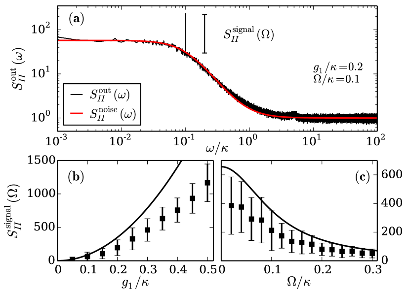
Figure 3: (Color online) Detection of weak force with a bistable OMS. (a) Spectral density for the homodyne photocurrent $S^{\text{out}}_{II}(\omega)$ in presence of a weak external force on the mechanical oscillator (black). The spectral density features a noise background and a signal peak. At small frequencies the noise background $S^{\text{noise}}_{II}(\omega)$ (red) can be approximated by a Lorentzian of width $\overline{W}$ at zero frequency, Eq. (23). (b) and (c) Signal peak height $S^{\text{signal}}_{II}(\Omega)=S_{II}^{\text{out}}(\Omega)-S_{II}^{\text{noise}}(\Omega)$ as a function of forcing amplitude $g_{1}$ (b) and forcing frequency $\Omega$ (c). Black squares are quantum trajectory simulations with statistical error bars. Black lines are analytical results based on the two-state rate equation model, Eq. (27), as discussed in the main text. The parameters are the same as in Fig. 1 but for $\Delta_{0}/\kappa=-1.4$. The weak external mechanical force has a frequency $\Omega/\kappa=0.1$ (a,b) and an amplitude $g_{1}/\kappa=0.2$ (a,c). The spectral density for each pair of parameters $(\Omega,g_{1})$ is obtained from an average over hundred spectra with a frequency resolution $\Delta\omega=10^{-3}\kappa$.

Describing the switching dynamics within the two-state rate equation model allows us to find analytic expressions for the low-frequency part of the output spectral density $S_{II}^{\text{out}}(\omega)$. As stated above, Eq. (18), $S_{II}^{\text{out}}(\omega)$ can be separated into a noise background $S_{II}^{\text{noise}}(\omega)$ and the signal part $S_{II}^{\text{signal}}(\omega)$.

In absence of the external force incoherent switching causes autocorrelations of the homodyne photocurrent to decay exponentially on a time scale $\overline{W}^{-1}$. We find the autocorrelation function (up to an irrelevant constant $I_{\text{ss}}^{2}$) is given by

$$\text{E}\left[I_{c}(t+\tau)I_{c}(t)\right]=e^{-\overline{W}|\tau|}\kappa p_{+}^{\text{ss}}p_{-}^{\text{ss}}(\bar{X}_{+}-\bar{X}_{-})^{2}+\delta(\tau)\>.$$ (22)

The second term stems from the shot noise of the local oscillator. The first term is proportional to the steady-state variance $\text{Var}(\hat{X})_{\text{ss}}=\langle\hat{X}^{2}\rangle_{\text{ss}}-\langle\hat{X}\rangle_{\text{ss}}^{2}\simeq p_{+}^{\text{ss}}p_{-}^{\text{ss}}(\bar{X}_{+}-\bar{X}_{-})^{2}$. Calculating $\text{Var}(\hat{X})_{\text{ss}}$ from the QME (7), we find that this two-state approximation overestimates the variance in the presence of appreciable intra-branch fluctuations around mean-field solutions. In fact, the noise background is smaller and more accurately given by

$$S_{II}^{\text{noise}}(\omega)=2\kappa\text{Var}(\textbf{:}\hat{X}\textbf{:})_{\text{ss}}\frac{\overline{W}}{\overline{W}^{2}+\omega^{2}}+1\>,$$ (23)

where $\text{Var}(\textbf{:}\hat{X}\textbf{:})_{\text{ss}}=\text{Var}(\hat{X})_{\text{ss}}-1$ is the normally-ordered variance of the amplitude quadrature, the colon denoting normal ordering of the optical creation and annihilation operators. Equation (23) satisfies the constraint that the total power of the homodyne photocurrent minus the shot-noise contribution must satisfy Wiseman and Milburn (1993), $\int[S_{II}^{\text{noise}}(\omega)-1]\frac{d\omega}{2\pi}=\kappa\text{Var}(\textbf{:}\hat{X}\textbf{:})_{\text{ss}}$. The noise spectrum consists of a shot noise contribution and a Lorentzian centered at zero frequency with a half width at half maximum given by $\overline{W}$.

Equation (17) allows us to find an approximate expression for the signal part $S_{II}^{\text{signal}}$ to the output spectral density. In the long-time limit a periodic time-dependence of the probability $p_{\pm}(t)$ yields a periodically modulated average homodyne photocurrent

$$\text{E}[I_{c}(t)] =\sqrt{\kappa}\left[p_{+}(t)\bar{X}_{+}+p_{-}(t)\bar{X}_{-}\right]$$ (24)

$$=I_{\text{ss}}+I(\Omega)\sin(\Omega t-\phi)$$

with the modulation amplitude in two-state approximation

$$I(\Omega)=\sqrt{\kappa}\left(\bar{X}_{+}-\bar{X}_{-}\right)\frac{W_{+}^{1}W_{-}^{0}-W_{-}^{1}W_{+}^{0}}{\overline{W}\sqrt{{\overline{W}}^{2}+\Omega^{2}}}\>.$$ (25)

The relationship between the average steady-state homodyne photocurrent $I_{\text{ss}}=\sqrt{\kappa}\langle\hat{X}\rangle_{\text{ss}}$, the probabilities $p_{\pm}^{\text{ss}}$, and the transitions rates $W_{\pm}^{i}$ given by Eqs. (11), (12), and (15) provide a direct interpretation of $I(\Omega)$. The zero-frequency expression $I(0)=(2g_{1}g_{0}/\omega_{m})(\partial I_{\text{ss}}/\partial\Delta_{0})$ is the linear response of $I_{\text{ss}}$ to a change in the detuning $\Delta_{0}$. The prefactor $2g_{1}/\omega_{m}$ is the zero-frequency response of the mechanical oscillator, i.e. the change in the mechanical equilibrium position (in units of its zero-point amplitude) caused by a static force with amplitude $g_{1}$. This displacement leads to a change of the cavity detuning $\Delta_{0}$ by $g_{0}(2g_{1}/\omega_{m})$. Relaxation of a bistable OMS at rate $\overline{W}$ causes an attenuation of this response at finite frequencies $\Omega$,

$$I(\Omega)=\frac{2g_{0}g_{1}}{\omega_{m}}\sqrt{\kappa}\frac{\partial\langle\hat{X}\rangle_{\text{ss}}}{\partial\Delta_{0}}\frac{\overline{W}}{\sqrt{\overline{W}^{2}+\Omega^{2}}}\>.$$ (26)

As stated in Eq. (19), the signal contributes a delta peak to the spectral density since the autocorrelation function of the homodyne photocurrent is dominated by periodic modulation in the limit $\tau\gg\overline{W}^{-1}$, and hence factorizes, $\text{E}[I_{c}(t+\tau)I_{c}(t)]=\text{E}[I_{c}(t+\tau)]\text{E}[I_{c}(t)]$. For a finite frequency resolution $\Delta\omega$,

$$S_{II}^{\text{signal}}(\Omega)=\frac{\pi\kappa}{2\Delta\omega}\left(\frac{2g_{1}g_{0}}{\omega_{m}}\frac{\partial\langle\hat{X}\rangle_{\text{ss}}}{\partial\Delta_{0}}\right)^{2}\frac{\overline{W}^{2}}{\overline{W}^{2}+\Omega^{2}}.$$ (27)

In Fig. 3(a) we plot the spectral density for the homodyne photocurrent $S^{\text{out}}_{II}(\omega)$ in the presence of a weak external force. An average over hundred spectra is shown. The spectral density features a low-frequency Lorentzian noise background whose frequency dependence agrees very well with our two-state approximation $S_{II}^{\text{noise}}(\omega)$, Eq. (23). The height of the signal peak relative to the noise level, $S_{II}^{\text{signal}}(\Omega)=S_{II}^{\text{out}}(\Omega)-S_{II}^{\text{noise}}(\Omega)$, is obtained for a range of forcing amplitudes $g_{1}$ and forcing frequencies $\Omega$. Comparing these quantum trajectory simulations to Eq. (27), we find that $S_{II}^{\text{signal}}(\Omega)$ exhibits the correct quadratic dependence on the forcing amplitude $g_{1}$ and Lorentzian dependence on the forcing frequency $\Omega$. The modulation amplitude $I(\Omega)$ is about 20% smaller than expected. We suspect that this quantitive disagreement is due to the large amplitude of intra-branch fluctuations reaching a considerable fraction of the inter-branch separation and the fact that the linear approximation to the modulation of switching rates (15) is only satisfied for the smaller values of $g_{1}$ in Fig. 3.

The expected power gain of a bistable OMS is

$$\mathcal{G}(\Omega)=\left(\frac{2g_{0}\kappa}{\omega_{m}}\frac{\partial\langle\hat{X}\rangle_{\text{ss}}}{\partial\Delta_{0}}\right)^{2}\frac{\overline{W}^{2}}{\overline{W}^{2}+\Omega^{2}}\>.$$ (28)

We notice that amplification occurs over a bandwidth given by the switching rate $\overline{W}$. As can be seen in Fig. 1(c), the slope $\partial\langle\hat{X}\rangle_{\text{ss}}/\partial\Delta_{0}$ in the center of the bistable region is approximately proportional to the difference between the two mean-field solutions $\bar{X}_{+}-\bar{X}_{-}$. As a consequence, a large difference in the cavity output fields leads to a strongly amplified homodyne signal. If the cavity is driven further away from bifurcation, the slope increases, but the switching rate $\overline{W}$ decreases. Thus, the gain can be made larger at the expense of reducing the bandwidth. For low signal frequency, $\Omega\lesssim\overline{W}$, for which the shot-noise contribution to the noise background $S_{II}^{\text{noise}}$ is negligible, the SNR is independent of $\Omega$,

$$\text{SNR}\simeq\pi\frac{\overline{W}}{\Delta\omega}\left(\frac{g_{1}g_{0}}{\omega_{m}}\right)^{2}\frac{\left(\partial\langle\hat{X}\rangle_{\text{ss}}/\partial\Delta_{0}\right)^{2}}{\text{Var}(\textbf{:}\hat{X}\textbf{:})_{\text{ss}}}+1\>,$$ (29)

with $\text{Var}(\textbf{:}\hat{X}\textbf{:})_{\text{ss}}$ and $(\partial\langle\hat{X}\rangle_{\text{ss}}/\partial\Delta_{0})^{2}$ obtained from Eq. (7). These two quantities have a similar dependence on the detuning $\Delta_{0}$ and reach their maximum at an optimal value of $\Delta_{0}$ in the center of the bistable region. As a consequence, both the SNR and the gain $\mathcal{G}$ are maximal.

Figure 4 shows the dimensionless signal output power $I(\Omega)^{2}/\kappa$ (a,b) and SNR (c,d) as a function of the signal input power $(g_{1}/\kappa)^{2}$ (a,c) and signal frequency $\Omega$ (b,d). We compare results from quantum trajectory simulations and from our two-state rate equation model. In panel (a) we see that the bistable OMS exihibits nearly constant power gain for small forcing amplitudes $g_{1}$. In panel (b) we observe that its detection bandwidth is in good agreement with predictions of the two-state model and given by the switching rate $\overline{W}$. As expected, the SNR is approximately constant over the detection bandwidth as can be seen in panel (c).

V.2 Force detection with an OMS in the linear regime

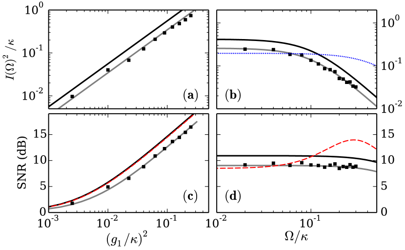
Figure 4: (Color online) Power gain and signal-to-noise ratio (SNR). Signal output power (a,b) and SNR (c,d) as function of the signal input power (a,c) and signal frequency (b,d). The expected values of $I(\Omega)^{2}$ and the SNR according to the two-state model discussed in the main text (black line) are compared to quantum trajectory results shown in Fig. 3 (black squares). Grey lines are a fit to the data indicating that the power gain $\mathcal{G}(\Omega)$ and the SNR have the correct dependence on the signal input power and signal frequency. The observed power gain has a value about 40% smaller than expected. In panel (b), the dotted blue line indicates the result for the largest possible power gain of an OMS operating in the linear regime $\mathcal{G}_{\text{lin}}^{\text{(max)}}$, Eq. (33). In panels (c) and (d), the dashed red line indicates the SNR for an OMS in the linear regime operating at the same power gain (extracted from the quantum trajectory results) and obtained from Eq. (36). The parameters are identical to Fig. 3, with an external forcing frequency $\Omega/\kappa=0.1$ (a,c) and amplitude $g_{1}/\kappa=0.2$ (b,d).

In the linear regime the dissipative dynamics of an OMS, including the noise and signal spectral densities of its output field quadratures, can be obtained exactly from the input-output formalism Gardiner and Collett (1985); Clerk et al. (2010). The linear regime is characterized by a small optomechanical coupling rate, $g_{0}\ll\kappa,\omega_{m}$, and a cavity driven to a coherent state with large amplitude $|\bar{a}|\gg 1$. Under these conditions, the radiation-pressure interaction can be approximated by a bilinear interaction, with an enhanced coupling rate $g=g_{0}|\bar{a}|$, between the resonator position, $\hat{b}+\hat{b}^{\dagger}$, and the amplitude quadrature, $\hat{a}+\hat{a}^{\dagger}$. The static shift of the resonator position results in an effective cavity detuning $\Delta=\Delta_{0}+g_{0}(\bar{b}+\bar{b}^{*})$. A displacement of the mechanical resonator imprints a phase shift on the output light field, which is best probed by driving the cavity on resonance, $\Delta=0$, and by measuring the phase quadrature at the output Aspelmeyer et al. (2013).

Analogous to Eq. (26) we find an expression for the amplitude modulation $I_{\text{lin}}$ and the spectral density $S_{II,\text{lin}}^{\text{signal}}$ of the phase quadrature in homodyne detection due to the force

$$\begin{gathered}I_{\text{lin}}(\Omega)=\sqrt{\mathcal{G}_{\text{lin}}(\Omega)}\frac{g_{1}}{\sqrt{\kappa}},\\ S_{II,\text{lin}}^{\text{signal}}(\omega)=\frac{\pi}{2}I_{\text{lin}}^{2}(\Omega)\left[\delta(\omega-\Omega)+\delta(\omega+\Omega)\right]\>.\end{gathered}$$ (30)

Here, the equivalent power gain at frequency $\omega$ for an OMS in the linear regime reads

$$\mathcal{G}_{\text{lin}}(\omega)=\left|2g\kappa\chi_{c}(\omega)\left[\chi_{m}(\omega)-\chi_{m}^{*}(\omega)\right]\right|^{2}\>,$$ (31)

with $\chi_{c}(\omega)=(\kappa/2-i\omega)^{-1}$ the cavity susceptibility and $\chi_{m}(\omega)=[\gamma_{m}/2+i(\omega_{m}-\omega)]^{-1}$ the mechanical susceptibility. The zero-frequency response can be written as $I_{\text{lin}}(0)=(2g_{0}g_{1}/\omega_{m})[\partial_{\Delta}(\sqrt{\kappa}\bar{I})]_{\Delta=0}$, i.e. the product of a shift of the cavity detuning caused by a static force with amplitude $g_{1}$ and the derivative with respect to $\Delta$ of the average homodyne photocurrent, $\sqrt{\kappa}\bar{I}$, where $\bar{I}=-i(\bar{a}-\bar{a}^{*})$ is the mean-field value of the optical phase quadrature and $\bar{a}=\epsilon/(\kappa/2-i\Delta)$. At low frequency, $\omega\ll\kappa,\omega_{m}$, the power gain is approximately constant,

$$\mathcal{G}_{\text{lin}}(\omega)=\left(\frac{2g_{0}\kappa}{\omega_{m}}\left[\frac{\partial\bar{I}}{\partial\Delta}\right]_{\Delta=0}\right)^{2}\>,$$ (32)

which is analogous to Eq. (28).

The low-frequency power gain, Eq. (32), can as well be expressed as $\mathcal{G}_{\text{lin}}(\omega)=(8g_{0}/\omega_{m})^{2}\bar{n}$, and is proportional to the average cavity occupation on resonance, $\bar{n}=|\bar{a}|^{2}=4(\epsilon/\kappa)^{2}$. An OMS can only operate in the linear regime below bifurcation, $\epsilon<\epsilon_{\text{bif}}$, that is for a cavity occupation below the critical value $n_{\text{bif}}=2\kappa\omega_{m}/(3\sqrt{3}g_{0}^{2})$. As a consequence, the power gain cannot be made arbitrarily large and the maximal gain has the universal value

$$\mathcal{G}_{\text{lin}}^{\text{(max)}}(\omega)\simeq\frac{128}{3\sqrt{3}}\frac{\kappa}{\omega_{m}}\>.$$ (33)

The spectral density of the noise interfering with the detection of a force signal far from the mechanical resonance, $|\omega-\omega_{m}|\gg\gamma_{m}$, referred back to the input signal is Clerk et al. (2010); Aspelmeyer et al. (2013)

$$\frac{S_{II,\text{lin}}^{\text{noise}}(\omega)}{\mathcal{G}_{\text{lin}}(\omega)}= \frac{1}{\mathcal{G}_{\text{lin}}(\omega)}+\mathcal{G}_{\text{lin}}(\omega)\frac{\left(\omega_{m}^{2}-\omega^{2}\right)^{2}}{16\kappa^{2}\omega_{m}^{2}}$$ (34)

$$+\left(n_{\text{th}}+\frac{1}{2}\right)\frac{\gamma_{m}}{\kappa}\frac{\omega^{2}+\omega_{m}^{2}}{2\omega_{m}^{2}}\>.$$

Equation (34) expresses the total measurement noise as fluctuations in the forcing amplitude and has three contributions. The first term is the imprecision noise due to the shot noise of the local oscillator. The second term is the back-action noise or radiation-pressure shot noise. The last term originates from thermal and quantum fluctuations of the resonator position.

At each frequency $\omega$, there is an optimal gain $\mathcal{G}_{\text{lin}}^{\text{(opt)}}(\omega)=2\kappa|\chi_{m}(\omega)-\chi_{m}^{*}(-\omega)|$ for which the measurement noise is minimal and the SNR maximal. In the limit of small frequencies, the optimal gain is then

$$\mathcal{G}_{\text{lin}}^{\text{(opt)}}\simeq\frac{4\kappa}{\omega_{m}}\>.$$ (35)

The low-frequency noise level for the optimal gain and a mechanical resonator coupled to a zero-temperature bath ($n_{\text{th}}=0$), $S_{II,\text{lin}}^{\text{noise}}\simeq 2+\gamma_{m}/\omega_{m}$, is minimal. This is commonly referred to as the standard quantum limit (SQL) of force (or position) detection. At the SQL the back-action noise and the imprecision noise are both equal to the shot-noise term.

V.3 Comparison of bistable and linear detection

An OMS in the regime of optical bistability exhibits a power gain $\mathcal{G}$ much larger than the gain $\mathcal{G}_{\text{lin}}$ of a linear OMS. The low-frequency expressions for the power gain of a bistable or linear OMS, Eqs. (28) and (32), depend on the coefficients $(\partial\langle\hat{X}\rangle_{\text{ss}}/\partial\Delta_{0})^{2}$ and $(\partial\bar{I}/\partial\Delta)^{2}$, respectively. These coefficients characterize the response of the steady-state value of the optical amplitude and phase quadratures, respectively, to a change in the detuning. The second coefficient is proportional to the average cavity occupation, which is limited by $\bar{n}<n_{\text{bif}}$. For a bistable OMS, $\partial\langle\hat{X}\rangle_{\text{ss}}/\partial\Delta_{0}$ is proportional to the difference between the mean-field solutions $\bar{X}_{+}-\bar{X}_{-}$ and can exceed $\partial\bar{I}/\partial\Delta$ far from the bifurcation. For small signal frequency $\Omega<\overline{W}$, the gain $\mathcal{G}(\Omega)$ is much larger than the optimal gain $\mathcal{G}_{\text{lin}}^{\text{(opt)}}(\Omega)$ at which the SQL applies, and can even be larger than $\mathcal{G}_{\text{lin}}^{\text{(max)}}(\Omega)$, i.e. the maximal gain for a linear OMS below bifurcation.

Figure 4(b) shows the dimensionless signal output power $I(\Omega)^{2}/\kappa$ as a function of the signal frequency $\Omega$ obtained from quantum trajectory simulations and from the two-state model. In addition, we indicate the results corresponding to a linear OMS operating at its maximal power gain $\mathcal{G}_{\text{lin}}^{\text{(max)}}$. Note that $\mathcal{G}(\Omega)>\mathcal{G}_{\text{lin}}^{\text{(max)}}(\Omega)$ within the detection bandwidth, i.e. for signal frequencies $\Omega\lesssim\overline{W}$.

As a consequence of the large gain $\mathcal{G}\gg\mathcal{G}_{\text{lin}}^{\text{(opt)}}$, the measurement noise $S_{II}^{\text{noise}}$ unavoidably exceeds the SQL value that applies to an OMS in the linear regime, $S_{II,\text{lin}}^{\text{noise}}\simeq 2+\gamma_{m}/\omega_{m}$. Thus, instead of comparing the sensitivity of our scheme to a linear OMS operating at the SQL, we compare it to the sensitivity of a linear OMS with identical gain. The SNR of a linear OMS can be expressed as a function of its power gain $\mathcal{G}_{\text{lin}}$ to compare it to results of quantum trajectory simulations. From Eqs. (30) and (34), we obtain, for small signal frequencies $\Omega\ll\kappa,\omega_{m}$ and $n_{\text{th}}=0$,

$$\text{SNR}=\frac{\pi g_{1}^{2}}{2\Delta\omega\kappa}\left[\frac{1}{\mathcal{G}_{\text{lin}}(\Omega)}+\mathcal{G}_{\text{lin}}(\Omega)\frac{\omega_{m}^{2}}{16\kappa^{2}}+\frac{\gamma_{m}}{4\kappa}\right]^{-1}.$$ (36)

In Fig. 4, we plot the SNR of a bistable OMS as function of the signal input power $(g_{1}/\kappa)^{2}$ (c) and signal frequency $\Omega$ (d). In addition, we plot the SNR of a linear OMS with identical parameters $\omega_{m}$, $\gamma_{m}$, and $\kappa$ and operating at the same gain $\mathcal{G}_{\text{lin}}(\Omega)=\mathcal{G}(\Omega)$, where $\mathcal{G}(\Omega)$ is extracted from quantum trajectory simulations. An important feature can be observed in panels (b) and (d) at signal frequencies in the detection bandwidth, $\Omega\lesssim\overline{W}$. The power gain of the bistable OMS exceeds $\mathcal{G}_{\text{lin}}^{\text{(max)}}$, while the SNR is still comparable to what is expected for a linear OMS with equal gain. Our results therefore indicate that large-gain force detection with an OMS can be realized beyond bifurcation, while preserving a sensitivity that is comparable to an equivalent linear OMS.

VI Conclusion

We have proposed bistable optomechanical systems as detectors of weak harmonic forces. An external mechanical force modulates the cavity frequency and thus the switching rates between the stable branches. A large difference in the respective optical output fields will thus lead to a strong amplification of the weak signal. The noise-induced switching dynamics in the presence of a harmonic force is described by a two-state rate equation model with periodically modulated switching rates. Using this model, we have calculated the output signal and noise spectral density relevant to homodyne detection of the optical field and compared them to quantum trajectory simulations. Finally, we have also compared the power gain and signal-to-noise ratio of our detection scheme to those of an optomechanical system in the linear regime. We find that a potentially larger gain can be achieved for low-frequency force signals while preserving comparable force detection sensitivity. These results point out a new direction for the use of optomechanical devices exhibiting an appreciable single-photon coupling rate for sensing applications requiring strong amplification.