Hot Jupiters from coplanar high-eccentricity migration.

Abstract

We study the possibility that hot Jupiters are formed through the secular gravitational interactions between two planets in eccentric orbits with relatively low mutual inclinations ($\lesssim 20^{\circ}$) and friction due to tides raised on the planet by the host star. We term this migration mechanism Coplanar High-eccentricity Migration because, like disk migration, it allows for migration to occur on the same plane in which the planets formed. Coplanar High-eccentricity Migration can operate from the following typical initial configurations: (i) inner planet in a circular orbit and the outer planet with an eccentricity $\gtrsim 0.67$ for $m_{\rm in}/m_{\rm out}(a_{\rm in}/a_{\rm out})^{1/2}\lesssim 0.3$; (ii) two eccentric ($\gtrsim 0.5$) orbits for $m_{\rm in}/m_{\rm out}(a_{\rm in}/a_{\rm out})^{1/2}\lesssim 0.16$. A population synthesis study of hierarchical systems of two giant planets using the observed eccentricity distribution of giant planets shows that Coplanar High-eccentricity Migration produces hot Jupiters with low stellar obliquities ($\lesssim 30^{\circ}$), with a semi-major axis distribution that matches the observations, and at a rate that can account for their observed occurrence. A different mechanism is needed to create large obliquity hot Jupiters, either a different migration channel or a mechanism that tilts the star or the proto-planetary disk. Coplanar High-eccentricity Migration predicts that hot Jupiters should have distant ($a\gtrsim 5$ AU) and massive (most likely $\sim 1-3$ more massive than the hot Jupiter) companions with relatively low mutual inclinations ($\lesssim 20^{\circ}$) and moderately high eccentricities ($e\sim 0.2-0.5$).

1. Introduction

At least $\sim 10-15\%$ of Sun-like stars harbor a Jovian-mass planet, while only $\sim 0.5-1\%$ harbor a so-called hot Jupiter (HJ) with semi-major axis $<0.1$ AU (Marcy et al., 2005; Gould et al., 2006; Mayor et al., 2011; Wright et al., 2012; Howard et al., 2012). Both radial velocity (RV) and transit surveys show that the HJs are piled up at a semi-major axis of $\sim 0.04-0.05$ AU (e.g., Hellier et al. 2012), and some of the HJs have significant eccentricities ($\sim 10\%$ have $e>0.2$) and stellar obliquities: $\sim 30\%$ of HJs have projected spin-orbit misalignment angle $\lambda>30^{\circ}$ as determined by Rossiter-MacLaughlin measurements.

Hot Jupiters could not have formed at their current locations because of the high gas temperature and low disk mass at these small radii (Bodenheimer et al., 2000). Instead, they must have formed beyond a few AU and then have migrated inwards, probably by angular momentum exchange with the protoplanetary disk (Goldreich & Tremaine, 1980; Ward, 1997) or by high-eccentricity migration (e.g., Rasio & Ford 1996; Wu & Murray 2003), in which the migrating planet attains very high eccentricities and tidal dissipation circularizes the orbit. Within the latter migration scenario, several different mechanisms to excite the eccentricity to high values have been proposed: the Kozai-Lidov mechanism in stellar binaries (Wu & Murray, 2003; Fabrycky & Tremaine, 2007; Naoz et al., 2012; Petrovich, 2015a), planet-planet scattering (Rasio & Ford, 1996; Nagasawa et al., 2008; Nagasawa & Ida, 2011; Beaugé & Nesvorný, 2012), and secular interactions between planets (Wu & Lithwick, 2011; Naoz et al., 2011). Although all of the migration mechanisms above can form hot Jupiters, which is the dominant channel (if any) remains an open question.

In this paper, we study the possibility that hot Jupiters are formed by the secular interaction of two planets in initially eccentric orbits in a hierarchical configuration ($a_{\rm in}\ll[1-e_{\rm out}]a_{\rm out}$) with relatively low mutual inclinations ($\lesssim 20^{\circ}$). We term this migration mechanism “Coplanar High-eccentricity Migration” (CHEM) to differentiate it from previously proposed high-eccentricity migration channels in which the eccentricity and inclination excitation generally go hand-in-hand (e.g., Nagasawa et al. 2008; Fabrycky & Tremaine 2007; Naoz et al. 2011).

Dynamically unstable multiple-planet systems generally relax into a long-term stable configuration with two planets in eccentric and hierarchical orbits (Weidenschilling & Marzari, 1996; Lin & Ida, 1997; Jurić & Tremaine, 2008; Chatterjee et al., 2008). The eccentricity distribution of these systems can reproduce the wide eccentricity distribution (median of $\simeq 0.23$) observed in the RV sample (Ford & Rasio, 2008; Jurić & Tremaine, 2008; Chatterjee et al., 2008). Planet-planet scattering does not only excite the planetary eccentricities, but it does also excite the planetary inclinations. However, in a significant fraction of the reported scattering experiments the planets end up in orbits with $e\gtrsim 0.5$ and mutual inclinations $\lesssim 20^{\circ}$ ($0.35$ radians), for which CHEM can operate (Timpe et al., 2013; Jurić & Tremaine, 2008; Chatterjee et al., 2008). In particular, Timpe et al. (2013) show that the mutual inclination of two surviving planets after planet-planet scattering in an initial three-planet system follows an exponential distribution with mean $\simeq 3.4^{\circ}-5.7^{\circ}$ ($\simeq 0.06-0.1$).

Various systems of two hierarchical planets on eccentric orbits are known to date. Kane & Raymond (2014) show that four known RV planets in multi-planet systems exhibit large amplitude secular eccentricity oscillations (inner planet reaches a maximum eccentricity $\sim 0.6-0.8$) and a stability analysis suggests that their (unknown) mutual inclinations are not too high so the inner planet avoids plunging into star. Similarly, Dawson et al. (2014) show that Kepler-419 is a hierarchical system ($a_{\rm in}=0.37$ AU, $a_{\rm out}=1.68$ AU) where the inner and outer planets have eccentricities of $\simeq 0.83$ and $\simeq 0.184$, respectively, while their mutual inclination is $9^{+8}_{-6}$ degrees.

The secular interaction between two planets in a hierarchical and coplanar configuration has been previously studied by several authors (e.g., Malhotra 2002; Lee & Peale 2003; Michtchenko & Malhotra 2004; Libert & Henrard 2005; Michtchenko et al. 2006; Migaszewski & Goździewski 2009). In particular, Lee & Peale (2003) and Michtchenko & Malhotra (2004) show that that the planetary orbits can engage in libration of $\varpi\equiv\varpi_{\rm in}-\varpi_{\rm out}$ around either $0^{\circ}$ or $180^{\circ}$, where $\varpi_{\rm in}$ and $\varpi_{\rm out}$ are the longitudes of pericenter of the inner and outer bodies. This libration can cause large amplitude eccentricity oscillations of either planet and, most important for this work, in some cases the inner planet might reach eccentricities large enough for friction due to tides raised on the planet by the host star to become important.

Similar to the previous work by Lee & Peale (2003) and Michtchenko & Malhotra (2004), Li et al. (2014a) recently studied the secular evolution of two hierarchical, nearly coplanar, and eccentric bodies, but in the test particle limit ($m_{\rm in}/m_{\rm out}\ll 1$). These authors confirmed that in this limit, the inner planet can reach unit eccentricity, derived a simple analytical condition for this to happen (see Eq. [5]), and showed that the orbit can flip its angular momentum vector to produce a coplanar retrograde planet.

Here, we extend these works by studying the conditions on the masses and the orbital elements in hierarchical and nearly coplanar planetary systems required to drive the eccentricities close to unity, and also by including the effects from general relativistic precession and tides that can limit the eccentricity growth.

2. Analytic results

In this section we use a time-averaged Hamiltonian of two hierarchical and nearly coplanar orbits expanded in series of the semi-major axis ratio to describe their secular evolution and assess which orbital elements and planetary masses allow for $e_{\rm in}\to 1$.

As discussed by Lee & Peale (2003) the coplanar problem has one degree of freedom: three variables ($e_{\rm in}$, $e_{\rm out}$, and $\varpi\equiv\varpi_{\rm in}-\varpi_{\rm out}$) and two conserved quantities (energy and total orbital angular momentum, Equations [LABEL:eq:potential] and [3]).

Hereafter, we shall use the notation from Petrovich (2015a) in which the variables are the eccentricity vectors ${\bf e}_{\rm in}$ and ${\bf e}_{\rm out}$, and the orbital angular momentum vectors ${\bf h}_{\rm in}$ and ${\bf h}_{\rm out}$ all defined in the Jacobi’s reference frame. We denote the masses of the central star and inner (outer) planets as $m_{1}$ and $m_{\rm in}$ ($m_{\rm out}$), respectively.

The double time averaged interaction potential in the octupole approximation (expansion up to $a_{\rm{in}}^{3}/a_{\rm{out}}^{4}$) is ${\phi}_{\rm oct}=\tilde{\phi}_{\rm{oct}}\phi_{0}$, where in the planetary limit ($m_{\rm in},m_{\rm out}\ll m_{1}$) we have (Petrovich, 2015a):

$$\tilde{\phi}_{\rm{oct}} = \frac{\phi_{\rm oct}}{\phi_{0}}=\frac{e_{\rm{in}}^{2}+2/3}{2(1-e_{\rm{out}}^{2})^{3/2}}-\frac{5\alpha}{16}\frac{3e_{\rm{in}}^{2}+4}{(1-e_{\rm{out}}^{2})^{5/2}}\bf{e}_{\rm{in}}\cdot\bf{e}_{\rm{out}},$$

with

$$\phi_{0}=\frac{3Gm_{\rm in}m_{\rm out}a_{\rm in}^{2}}{4a_{\rm out}^{3}},$$ (2)

$\alpha=a_{\rm in}/a_{\rm out}$, and $\bf{\hat{e}}_{\rm{in}}\cdot\bf{\hat{e}}_{\rm{out}}=\cos\varpi$.

This potential is accurate to first order in the mutual inclination $i_{\rm tot}$ with $\cos i_{\rm tot}=\hat{{\bf h}}_{\rm in}\cdot\hat{{\bf h}}_{\rm out}$ and it has proven to be very accurate for $\alpha\lesssim 0.1$ in the planetary limit (Lee & Peale, 2003). Note that this interaction potential has positive energy—the opposite sign as the standard definition of the interaction Hamiltonian.

Similarly, we define the ratio between the total orbital angular momentum and the total orbital angular momentum that would obtain if the orbits were circular as

$$\mathcal{J}=\frac{\mu\alpha^{1/2}(1-e_{\rm{in}}^{2})^{1/2}+(1-e_{\rm{out}}^{2})^{1/2}}{\mu\alpha^{1/2}+1},$$ (3)

where $\mu$ is the planetary mass ratio $\mu=m_{\rm in}/m_{\rm out}$.

The quantity $\mathcal{J}$ is a constant of motion in the secular approximation and in the absence of extra forces other than the gravitational interactions between the planets and the star. This result immediately implies that for a given $\mathcal{J}$ we have

$$e_{\rm in}\leq\sqrt{1-\left[\frac{(1+\mu\alpha^{1/2})\mathcal{J}-1}{\mu\alpha^{1/2}}\right]^{2}}$$ (4)

if $(1+\mu\alpha^{1/2})\mathcal{J}\geq 1$, while $e_{\rm in}$ can reach unity if $(1+\mu\alpha^{1/2})\mathcal{J}\leq 1$ (set $e_{\rm in}=1$ and $e_{\rm out}\geq 0$ in Eq. [3]).

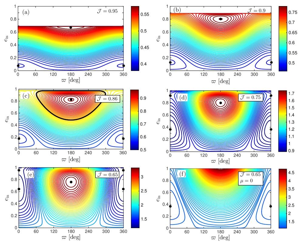
Figure 1.— Level curves of the dimensionless potential $\tilde{\phi}_{\rm oct}$ (Eq. LABEL:eq:potential) for different values of $\mathcal{J}$ (Eq. 3) as indicated in each panel. In panels a-e we fix $\alpha\equiv a_{\rm in}/a_{\rm out}=1/8$ and $\mu\equiv m_{\rm in}/m_{\rm out}=0.606$ as in the example in Figure 5, and in panel c we show the trajectory with $\mathcal{J}=0.86$ and $\tilde{\phi}_{\rm oct}=0.83$ that corresponds to the initial condition of that example (black thick line). In panel f we show the test particle limit $\mu=0$ with $\alpha=1/8$ and $\mathcal{J}=0.65$. The black dots indicate the fixed points of $de_{\rm in}/dt=d\varpi/dt=0$ from Equations (22) and (24).

2.1. Phase-space trajectories

In Figure 1 we show level curves of the dimensionless potential $\tilde{\phi}_{\rm oct}$ in Equation (LABEL:eq:potential) for different values of the dimensionless total orbital angular momentum $\mathcal{J}$ in Equation (3). From panels a to e, we fix the planetary mass ratio to $\mu=0.606$ and the semi-major axis ratio to $\alpha=1/8$, similar to our example in Figure 5. For these parameters $e_{\rm in}$ can reach unity if $\mathcal{J}\leq 0.824$. In panel f we show the test particle limit $\mu=0$ with $\alpha=1/8$ and $\mathcal{J}=0.65$. In all panels, we indicate the fixed points $de_{\rm in}/dt=d\varpi/dt=0$ from Equations (22) and (24) as black circles.

From panel a, we observe that for $\mathcal{J}=0.95$ the phase-space trajectories are restricted to $e_{\rm in}\leq 0.697$ as required from Equation (4). Most trajectories correspond to circulation of the relative apsidal angle $\varpi$ and the minimum eccentricities happen at $\varpi=180^{\circ}$ (anti-parallel eccentricity vectors). The eccentricity variation between $\varpi=180^{\circ}$ and $\varpi=0$ (or $\varpi=360^{\circ}$) is at most $\sim 0.15$. There are two fixed points of the equations of motions (solutions to $de_{\rm in}/dt=d\varpi/dt=0$ in Equations [22] and [24]): one at $\varpi=0$ and $e_{\rm in}=0.0782$ with low energy ($\tilde{\phi}_{\rm oct}=0.405$), and another at $\varpi=180^{\circ}$ and $e_{\rm in}=0.681$ with high energy ($\tilde{\phi}_{\rm oct}=0.591$). Close to these fixed points the trajectories correspond to librations of $\varpi$ and the eccentricity, as previously identified by Lee & Peale (2003).

By decreasing the total orbital angular momentum from $\mathcal{J}=0.95$ to $\mathcal{J}=0.9$ (panel b), the fixed point at $\varpi=180^{\circ}$ moves from $e_{\rm in}=0.681$ to $e_{\rm in}=0.81$, while that at $\varpi=0$ moves from $e_{\rm in}=0.0782$ to $e_{\rm in}=0.128$. The libration region around these two fixed points occupies a larger volume in $e_{\rm in}-\varpi$ space relative to that when $\mathcal{J}=0.95$. The angular momentum constraint in Equation (4) limits the eccentricity to $e_{\rm in}<0.901$.

In panel c, we decrease the angular momentum even further to $\mathcal{J}=0.86$ (panel c), which allows for a maximum eccentricity $e_{\rm in}=0.978$ (Eq. [4]). The parameters in this panel are chosen to coincide with the initial conditions from our example in Figure 5 in which the inner planet undergoes migration. That phase-space trajectory in this example is indicated by the black thick line and it corresponds to large amplitude eccentricity librations in the range $e_{\rm in}\simeq 0.5-0.98$ and $\varpi$ in $\simeq 60^{\circ}-300^{\circ}$. We note that for the energy levels close to our example ($\tilde{\phi}_{\rm oct}\sim 0.8$) there are trajectories that could lead to eccentricities close to unity from either circulation or libration of $\varpi$.

In panel d we set $\mathcal{J}=0.75$ and observe that most trajectories with $\tilde{\phi}_{\rm oct}\lesssim 1.6$ pass through $e_{\rm in}\simeq 1$. Even if one starts from a circular orbit and $\varpi\sim 100^{\circ}-260^{\circ}$ the eccentricity of the inner planet always attains very high values. Also, we observe that there are two fixed points at $\varpi=0$: one at $e_{\rm in}=0.359$ and the other at $e_{\rm in}=0.922$. The former corresponds to a stable fix point around which $\varpi$ librates with possibly large amplitude eccentricity oscillations, while the latter is unstable (a saddle point) and it only appears when $\mathcal{J}<0.845$.

In panel e we set $\mathcal{J}=0.65$. By decreasing $\mathcal{J}$ from 0.75 to 0.65 we observe that the fixed points at $\varpi=0$ move to higher values and that the trajectories starting from circular orbits can reach unity eccentricities for all values of $\varpi$.

In panel f we show the test particle limit $\mu=0$ for $\mathcal{J}=0.65$ (or $e_{\rm out}$=0.76 from Eq. [3]) and observe that there is only one fixed point at $\varpi=0$ and $e_{\rm in}=0.365$. Consistently, from Equation (24) one can easily show that for all values of $\mathcal{J}$ there is no physical solution for $d\varpi/dt=0$ when $\varpi=180^{\circ}$. Similarly, there is only one physical solution when $\varpi=0$, which is given by $e_{\rm in}=\left(1-\sqrt{1-4\beta^{2}}\right)/(3\beta)$ with $\beta=15\alpha\sqrt{1-\mathcal{J}^{2}}/(8\mathcal{J})$. This result implies that in the test particle approximation there can be only libration of $\varpi$ and $e_{\rm in}$ around one fixed point at $\varpi=0$.

In summary, the secular phase-space trajectories of two hierarchical and coplanar orbits include circulation of $\varpi$ and also libration of $\varpi$ around $0$ and $180^{\circ}$. Both the circulating and the librating trajectories around $180^{\circ}$ can lead to very high values of $e_{\rm in}$. In the test particle approximation the libration of $\varpi$ around $180^{\circ}$ is not present.

2.2. Available phase-space for migration

Hereafter, we use the subscripts $i$ and $f$ to denote the initial and final states.

In the test particle approximation, $e_{\rm out}$ is constant and Equation (LABEL:eq:potential) implies that $e_{{\rm in},f}\to 1$ only if

$$\alpha\frac{e_{\rm out}}{1-e_{\rm out}^{2}}=\frac{8}{5}\frac{1-e_{{\rm in},i}^{2}}{7\cos\varpi_{f}-e_{{\rm in},i}(4+3e_{{\rm in},i}^{2})\cos\varpi_{i}},$$ (5)

which translates into the condition of Li et al. (2014a) (Equation 14 therein) since $\cos\varpi_{f}\leq 1$.

In what follows, we do not assume that the inner planet is a test particle.

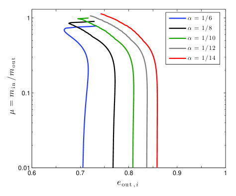
Figure 2.— Solutions to Equation (7) as a function of the initial eccentricity of the outer planet $e_{{\rm out},i}$ and the planetary mass ratio $\mu=m_{\rm in}/m_{\rm out}$ (see text). The color label indicates different values of the semi-major axis ratio $\alpha=\{1/6,1/8,1/10,1/12,1/14\}$. The solutions correspond to the minimum eccentricity of the outer planet that is required for the inner planet to increase its eccentricity from 0 to 1 for a given value of $\mu$.

2.2.1 Initial circular orbit

Let us start by assuming that in the initial state $e_{{\rm in},i}=0$ and it reaches a final state with $e_{{\rm in},f}\to 1$. Thus, the energy conservation in Equation (LABEL:eq:potential) implies

$$\frac{1}{3(1-e_{{\rm out},i}^{2})^{3/2}} = \frac{5}{6(1-e_{{\rm out},f}^{2})^{3/2}}$$ (6)

$$- \frac{35\alpha}{16}\frac{e_{{\rm out},f}}{(1-e_{{\rm out},f}^{2})^{5/2}}\cos\varpi_{f},$$

and by using $\mu\alpha^{1/2}+(1-e_{{\rm out},i}^{2})^{1/2}=(1-e_{{\rm out},f}^{2})^{1/2}$ we get a condition for $e_{{\rm out},i}$, $\mu$, $\varpi_{f}$, and $\alpha$, as:

$$\frac{1}{3(1-e_{{\rm out},i}^{2})^{3/2}}=\frac{5}{6\left[\mu\alpha^{1/2}+(1-e_{{\rm out},i}^{2})^{1/2}\right]^{3}}$$

$$-\frac{35\alpha}{16}\frac{\left\{1-\left[\mu\alpha^{1/2}+(1-e_{{\rm out},i}^{2})^{1/2}\right]^{2}\right\}^{1/2}}{\left[\mu\alpha^{1/2}+(1-e_{{\rm out},i}^{2})^{1/2}\right]^{5}}\cos\varpi_{f},$$ (7)

where we note that the minimum (maximum) value of $e_{{\rm out},i}$ required to solve this equation is given by $\varpi_{f}=0$ ($\varpi_{f}=\pi$). However, it can happen that a phase-space trajectory connecting $e_{{\rm in},i}=0$ with $e_{{\rm in},f}\to 1$ and $\varpi_{f}=0$ might not exist. Thus, in order to find the minimum outer eccentricity to reach $e_{{\rm in},f}\to 1$ we numerically find the minimum value of $\varpi_{f}$ (if any) that connects $e_{\rm in}=0$ with $e_{\rm in}=1$, while satisfying Equation (7). As an example, from panel d in Figure 1 the path that connects $e_{\rm in}=0$ with $e_{\rm in}=1$ has $\varpi_{f}\simeq 50^{\circ}$.

We proceed as follows. For each combination of $\mu$ and $\alpha$ we solve the Equation (7) starting with $\varpi_{f}=0$ and check if the phase-space trajectory is continuous. If the trajectory is continuous, then we have determined the minimum eccentricity of the outer planet to reach $e_{{\rm in},f}\to 1$. If trajectory is not continuous, we increase $\varpi_{f}$ and repeat the procedure until we find a continuous path (if any) with $\varpi_{f}=0-180^{\circ}$.

In Figure 2 we show our results for the minimum initial eccentricity of the outer planet $e_{{\rm out},i,{\rm min}}$ to excite $e_{\rm in}$ from 0 to 1 as a function of the planetary mass ratio $\mu$ and for different values of the semi-major axis ratio $\alpha$. We observe that for a fix value of $\alpha$, $e_{{\rm out},i,{\rm min}}$ reaches its lowest value of $\sim 0.67-0.75$ for $\mu\sim 0.7-1$, while it increases almost monotonically for lower values of $\mu$. Similarly, $e_{{\rm out},i,{\rm min}}$ increases as $\alpha$ decreases. We describe these observations below.

In the test particle approximation the trajectories connecting $e_{{\rm in},i}=0$ with $e_{{\rm in},f}=1$ are all continuous (the fixed point at $\varpi=0$ and high $e_{\rm in}$ disappears), implying that the minimum $\varpi_{f}$ is 0 (see panel f in Figure 1). Thus, by setting $\varpi_{f}=0$ in Equation (6) the minimum eccentricity $e_{{\rm out},i,{\rm min}}$ in the test particle approximation (constant $e_{\rm out}$) is given by

$$e_{{\rm out},i,{\rm min}}=\frac{\sqrt{1+\gamma^{2}}-1}{\gamma},$$ (8)

where $\gamma=16/(35\alpha)$.

When the inner and outer masses are comparable, the the eccentricity of the outer planet can change. We can calculate $e_{{\rm out},i,{\rm min}}$ from the limiting case in which $e_{{\rm out},f}=0$: the inner orbit transfers the maximum angular momentum possible to the outer orbit. Thus, by setting $e_{{\rm out},f}=0$ in Equation (6) we obtain

$$e_{{\rm out},i,{\rm min}}=\sqrt{1-\left(2/5\right)^{2/3}}=0.676,$$ (9)

which roughly coincides with the lowest values of $e_{{\rm out},i,{\rm min}}$ in Figure 2 for $\mu\sim 0.7-1$ and $\alpha\leq 1/10$.

The values of $\mu$ and $\alpha$ at which $e_{{\rm out},i,{\rm min}}$ is lowest can be estimated by setting $e_{{\rm out},i,{\rm min}}=0.676$ and $e_{{\rm out},f}=0$ in the angular momentum conservation condition, which results in $\mu\alpha^{1/2}=1-\left(2/5\right)^{1/3}=0.263$. This value is only an estimate and we numerically find that $0.3$ approximates better than $0.263$ the position of the minimum $e_{{\rm out},i,{\rm min}}$ in Figure 2. Thus, we conclude from this analysis that the parameters required to excite the eccentricity of the inner planet from zero to unity with the lowest eccentricities of the outer planet should satisfy:

$$\mu\alpha^{1/2}\equiv\frac{m_{\rm in}}{m_{\rm out}}\left(\frac{a_{\rm in}}{a_{\rm out}}\right)^{1/2}\simeq 0.3.$$ (10)

For $\mu\alpha^{1/2}\gtrsim 0.3$ there are no solutions to Equation (6), while for $\mu\alpha^{1/2}\lesssim 0.3$ the required eccentricities increase with decreasing $\mu\alpha^{1/2}$ until they reach the test particle limit ($\mu\ll 1$), which is given by Equation (8).

We note that given the high values of $e_{{\rm out},i}$ required to reach $e_{\rm in}\to 1$, starting from a circular orbit might cause the system to become dynamically unstable. According to the stability boundary of hierarchical triple systems from Mardling & Aarseth (2001) (Eq. [26]), a planetary system ($m_{\rm in},m_{\rm out}\ll m_{1}$) with an outer eccentricity of $e_{\rm out}=0.676$ is stable for $\alpha<1/13.3$. Thus, if the systems with $\alpha>1/13.3$ were indeed unstable the available phase-space for migration starting from an inner circular orbit would be strongly limited. However, in a recent work Petrovich (2015b) shows that most systems with $m_{\rm in}\sim m_{\rm out}\sim 1M_{J}$, $e_{\rm in}\sim 0$ and $e_{\rm out}\simeq 0.7$ are long-term stable for $\alpha\lesssim 1/8$. We adopt this less conservative stability limit for our discussion in §4.5.

In summary, the eccentricity excitation of the inner planet from a circular to a radial orbit is possible only if the outer body starts from an eccentric orbit with $e_{\rm out}\gtrsim 0.67$ and the mass and semi-major axis ratios satisfy $\mu\alpha^{1/2}\lesssim 0.3$. As $\mu\alpha^{1/2}$ departs from 0.3 the required eccentricities of the outer planet increase, implying that the eccentricity excitation is most efficient for planets of comparable masses with $\mu=m_{\rm in}/m_{\rm out}\sim 0.7-1$.

2.2.2 Initial eccentric orbit

We now relax the requirement that the inner planet is initially in a circular orbit. Thus, we use the conservation of energy in Equation (LABEL:eq:potential) and only fix $\varpi_{i}=\pi$ as

$$\tilde{\phi}_{\rm{oct}}(e_{{\rm in},i},e_{{\rm out},i},\varpi_{i}=\pi)=\tilde{\phi}_{\rm{oct}}(e_{{\rm in},f}=1,e_{{\rm out},f},\varpi_{f}),$$

(11)

which can be numerically solved along with the angular momentum conservation condition in Equation (3) for different values of of $e_{{\rm in},i}$ and $\varpi_{f}$.

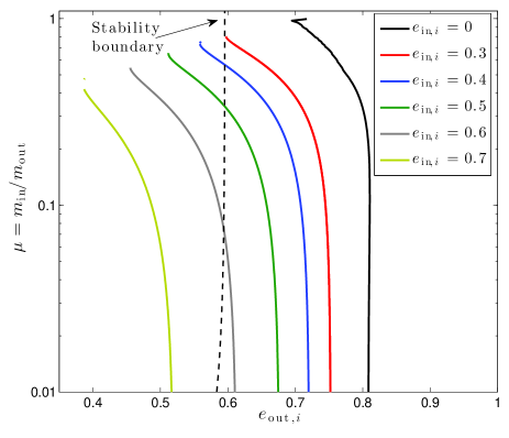
Figure 3.— Solutions to Equation (11) as a function of the initial eccentricity of the outer planet $e_{{\rm out},i}$ and the planetary mass ratio $\mu=m_{\rm in}/m_{\rm out}$, for a fixed semi-major axis ratio $\alpha=1/10$. The color labels indicate different values of the initial eccentricity of the inner planet $e_{{\rm in},i}$. The solutions correspond to the minimum eccentricity of the outer planet that is required for the inner planet to increase its eccentricity from $e_{{\rm in},i}$ to 1 for a given value of $\mu$. The stability boundary for hierarchical triple systems from Equation (26) is indicated as a dashed black line (stable configurations are left to the line).

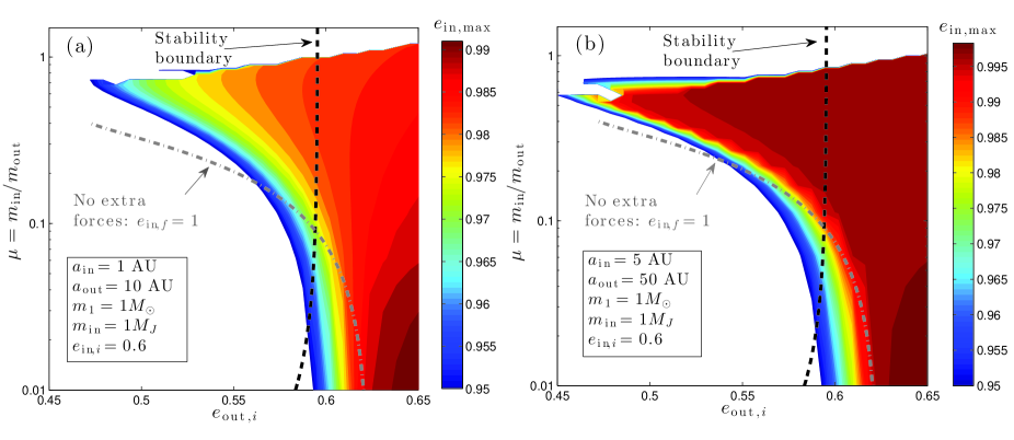
Figure 4.— Contour levels of the maximum eccentricity of the inner planet as a function of $e_{{\rm out},i}$ and the mass ratio $\mu=m_{\rm in}/m_{\rm out}$ obtained from Equations (3) and (19), which include the extra forces from general relativity and the tidal quadrupole. We fix the initial eccentricity of the inner planet to $e_{{\rm in},i}=0.6$ and the masses of the star and the inner planet to $m_{1}=1M_{\odot}$ and $m_{\rm in}=1M_{J}$, respectively. Panel a: the semi-major axes of the inner and outer planets are $a_{\rm in}=1$ AU and $a_{\rm out}=10$ AU. Panel b: the semi-major axes of the inner and outer planets are $a_{\rm in}=5$ AU and $a_{\rm out}=50$ AU. The stability boundary from Equation (26) is shown as the dashed black line. The minimum initial eccentricity of the outer planet required to reach $e_{\rm in}=1$ when no extra forces are included (Eq. [11]) is shown as the dot-dashed gray line.

In Figure 3 we show the roots of Equation (11) numerically minimizing the outer eccentricity $e_{{\rm out},i}$ over $\varpi_{f}$ restricted to continuous phase-space trajectories (see §2.2.1) for different values of the initial eccentricity of the inner planet. For a given mass ratio $\mu$ each curve indicates the minimum eccentricity of the outer planet that is required to excite the eccentricity of the inner planet from $e_{{\rm in},i}$ to $1$.

Not surprisingly, we observe from this figure that by starting from higher initial eccentricities of the inner planet we require smaller eccentricities of the outer planet to reach $e_{{\rm in},f}\simeq 1$, as expected. Also, as we increase $e_{{\rm in},i}$ the maximum mass ratio $\mu$ at which the eccentricity excitation can happen is lower and the minimum values of the outer eccentricity $e_{{\rm out},i}$ are reached when $\mu\sim 0.3-1$.

The analysis can be further simplified by assuming that initially the eccentricities of inner and outer planets are equal: $e_{{\rm in},i}=e_{{\rm out},i}$. This is an arbitrary assumption that we use to derive analytical expressions. Similar to the previous section, we can determine the initial minimum eccentricity (of the inner and outer planets) $e_{{\rm min}}$ required to reach $e_{{\rm in},f}\to 1$ by observing that the maximum angular momentum transfer from the inner to the outer orbit occurs when $e_{{\rm out},f}\to 0$. Replacing these limits in Equation (11), we get

$$\frac{e_{\rm{min}}^{2}+2/3}{2(1-e_{\rm{min}}^{2})^{3/2}}+\frac{5\alpha}{16}\frac{(3e_{\rm{min}}^{2}+4)e_{\rm{min}}^{2}}{(1-e_{\rm{min}}^{2})^{5/2}}=\frac{5}{6};$$ (12)

in the limit $\alpha\to 0$ the zero of this equation is $e_{\rm{min}}=0.55$. Moreover, we can find the largest value $\alpha$ such that the pair $\{\alpha,e_{\rm{min}}\}$ satisfies both Equation (12) and the stability condition in Equation (26). We numerically find that the solution is $\alpha=1/7.8$ and $e_{\rm{min}}=0.51$. In other words, for planetary systems with initial equal inner and outer eccentricities and in dynamically stable configurations, the required eccentricity and semi-major axis ratio to reach $e_{{\rm in},f}\to 1$ are $e_{{\rm in},i}=e_{{\rm out},i}\geq 0.51$ and $\alpha<1/7.8$, respectively.

By replacing $e_{{\rm in},i}=e_{{\rm out},i}=0.51$ in the angular momentum conservation condition (Eq. [3]) we get that the required values of $\mu$ and $\alpha$ to reach $e_{{\rm in},f}\to 1$ with the minimum inner and outer eccentricities are

$$\mu\alpha^{1/2}=\frac{1}{(1-0.51^{2})^{1/2}}-1=0.162,$$ (13)

where $\alpha<1/7.8$ and $\mu>0.45$. In a recent work Petrovich (2015b) shows that the stability condition in Equation (26) is somewhat conservative and many systems with $\alpha<1/7.8$ are likely to be long-term stable. His results indicate that two Jupiter-mass planets with eccentricities of 0.5 are long-term stable for $\alpha\lesssim 1/5$. By using these findings by Petrovich (2015b) the conditions on the semi-major axis ratio and mass ratio change to $\alpha\lesssim 1/5$ and $\mu\gtrsim 0.36$, while the minimum eccentricities change only slightly from 0.51 to 0.49.

Consistent with our example in Figure 5, which has a planetary mass ratio of $\mu=2M_{J}/(3.3M_{J})=0.606$ and initial eccentricities of $e_{{\rm in},i}=e_{{\rm in},f}=0.51$, we observe from Figure 3 that starting from $e_{{\rm in},i}=0.5$ (green line) we can reach very high eccentricities for $\mu\simeq 0.6$ and $e_{{\rm out},i}\simeq 0.5$. Similarly, the condition in Equation (13) for $\alpha=1/8$ results in $\mu=0.458$, roughly consistent with the example in Figure 5.

In summary, the required eccentricity of the outer planet to excite the eccentricity of the inner planet up to unity decreases with the initial inner eccentricity and it reaches a minimum for planetary mass ratios $\mu\sim 0.3-1$ when $\alpha=1/10$. When both planets start with the same eccentricity, the minimum required initial eccentricities are $\simeq 0.5$, while the dynamical stability of the system requires that the semi-major axis ratio is $\alpha\lesssim 1/5$ and the mass ratio is $\mu=m_{\rm in}/m_{\rm out}\gtrsim 0.36$.

2.3. Extra forces and maximum eccentricity growth

We study the effect that extra forces have on the three-body system considered here and how they limit the eccentricity growth. We do this by including extra terms in the orbit-averaged dimensionless potential $\tilde{\phi}_{\rm oct}$ in Equation (LABEL:eq:potential). For consistency with the positive sign in our definition of $\tilde{\phi}_{\rm oct}$, we also define the interaction potentials as positive below.

The first order general relativistic (GR) correction in the planetary approximation ($m_{\rm in},m_{\rm out}\ll m_{1}$) can be written in a dimensionless form as:

$$\tilde{\phi}_{\rm{GR}} = \frac{\phi_{\rm{GR}}}{\phi_{0}}=\frac{4Gm_{1}^{2}}{c^{2}a_{\rm in}m_{\rm in}}\mu\alpha^{-3}\left(1-e_{\rm{in}}^{2}\right)^{-1/2},$$ (14)

where by setting $m_{1}=1M_{\odot}$ and $m_{\rm in}=1M_{J}$, we get

$$\tilde{\phi}_{\rm{GR}} = 0.0396\left(\frac{1~{}{\rm AU}}{a_{\rm in}}\right)\mu\left(\frac{0.1}{\alpha}\right)^{3}\left(1-e_{\rm{in}}^{2}\right)^{-1/2}.$$ (15)

Similarly, the dimensionless potential due to the tidal quadrupole on the planet can be written as (e.g., Fabrycky & Tremaine 2007)

$$\tilde{\phi}_{\rm{tq}}=\frac{\phi_{\rm{tidal}}}{\phi_{0}} = \frac{4k_{p}}{3}\left(\frac{m_{1}}{m_{\rm in}}\right)^{2}\left(\frac{R_{\rm in}}{a_{\rm in}}\right)^{5}\mu\alpha^{-3}$$ (16)

$$\times\frac{1+3e_{\rm{in}}^{2}+3e_{\rm{in}}^{4}/8}{(1-e_{\rm{in}}^{2})^{9/2}},$$

where for $m_{1}=1M_{\odot}$, $m_{\rm in}=1M_{J}$, a tidal Love number of the planet of $k_{p}=0.26$, and radius of the inner planet $R_{\rm in}=R_{J}$, we get

$$\tilde{\phi}_{\rm{tq}}=\frac{\phi_{\rm{tidal}}}{\phi_{0}} = 7.93\times 10^{-9}\left(\frac{1\mbox{ AU}}{a_{\rm in}}\right)^{5}\mu\left(\frac{0.1}{\alpha}\right)^{3}$$ (17)

$$\times\frac{1+3e_{\rm{in}}^{2}+3e_{\rm{in}}^{4}/8}{(1-e_{\rm{in}}^{2})^{9/2}}.$$

We note that with these parameters both GR and tidal quadrupole contributions can become comparable to $\tilde{\phi}_{\rm oct}$ in Equation (LABEL:eq:potential), which is of order unity, only at very high eccentricities or small semi-major axis $a_{\rm in}$. For the parameters in Equations (15) and (17) we get that $\tilde{\phi}_{\rm{GR}}=\tilde{\phi}_{\rm{tq}}$ at eccentricities of $e_{\rm in}\simeq 0.983$. For $e_{\rm in}<0.983$ GR dominates over the tidal bulge, while the opposite happens for $e_{\rm in}>0.983$.

We write the dimensionless potential that includes the extra forces as:

$$\tilde{\phi}_{\rm{extra}}\equiv\tilde{\phi}_{\rm{oct}}+\tilde{\phi}_{\rm{GR}}+\tilde{\phi}_{\rm{tq}}.$$ (18)

In Figure 4 we show the maximum eccentricity of the inner planet as a function of $e_{{\rm out},i}$ and the mass ratio $\mu=m_{\rm in}/m_{\rm out}$ from solving the equation:

$$\tilde{\phi}_{\rm{extra}}(e_{\rm in,i},e_{\rm out,i},\varpi_{i}=\pi)=\tilde{\phi}_{\rm{extra}}(e_{\rm in,f},e_{\rm out,f},\varpi_{f}),$$ (19)

where we fix the initial eccentricity of the inner planet to $e_{{\rm in},i}=0.6$ and the masses of the star and the inner planet to $m_{1}=1M_{\odot}$ and $m_{\rm in}=1M_{J}$, respectively. By using the total angular momentum conservation (Eq. [3]) we can solve for $e_{{\rm in},f}$ (or $e_{{\rm out},f}$) and $\varpi_{f}$. The maximum eccentricity of the inner planet is obtained by numerically maximizing over $\varpi_{f}$.

In panel a, we show our results for $a_{\rm in}=1$ AU and $a_{\rm out}=10$ AU. We observe that the maximum eccentricity is limited (i.e., $e_{{\rm in},f}<1$) by the inclusion of the extra forces. For comparison we show the minimum $e_{{\rm out},i}$ required to reach $e_{{\rm in},f}=1$ (similar to Figure 3) when no extra forces are included (dot-dashed gray line). We observe that the extra forces limit the maximum eccentricity more efficiently for larger values of $\mu=m_{\rm in}/m_{\rm out}$. For instance, for $\mu=0.01$ (0.4) we get that $e_{{\rm in},f}=1$ with no extra forces and a minimum $e_{{\rm out},i}\simeq 0.62$ ($\simeq 0.47$ ), while for the same value of $e_{{\rm out},i}$ the extra forces yield a maximum eccentricity of $\simeq 0.99$ ($<0.95$). This is because for more massive outer perturbers both $\tilde{\phi}_{\rm{GR}}$ and $\tilde{\phi}_{\rm{tq}}$ are smaller: the extra forces do not depend on the mass of the perturber, while the point-like gravitational interactions increase linearly in magnitude with $m_{\rm out}$.

From panel a, we note that the maximum eccentricity the inner orbit can reach is always less than $\simeq 0.985$ for dynamically stable configurations (left of the stability boundary, dashed black line). This result implies that the pericenter distance is $r_{p}\equiv a_{\rm in}(1-e_{\rm in})>0.015$ AU and, therefore, no tidal disruptions are expected for these parameters. Moreover, if the planets undergo migration at roughly constant angular momentum then their final semi-major axis is roughly twice the minimum pericenter distance, which implies that the semi-major axes of the hot Jupiters are constrained to $a>0.03$ AU.

In panel b, we show our results for $a_{\rm in}=5$ AU and $a_{\rm out}=50$ AU. We observe that the maximum eccentricity is higher than that with $a_{\rm in}=1$ AU (panel a), which is expected because both $\tilde{\phi}_{\rm{GR}}$ and $\tilde{\phi}_{\rm{tq}}$ decrease with $a_{\rm in}$, while $\tilde{\phi}_{\rm{oct}}$ remains constant (at fixed $\alpha$). In particular, we observe that a large fraction of the area displayed in the plot reaches a maximum eccentricity of $\simeq 0.995$ (in dark red).

By only considering that GR as an extra force, we can roughly estimate the dependence of the maximum eccentricity on $a_{\rm in}$ from Equation (19) by using that in the initial state $\tilde{\phi}_{\rm{GR}}\ll\tilde{\phi}_{\rm{oct}}$ (initial eccentricity is not too high or $a_{\rm in}$ is not too small) and that in the final state with $1-e_{\rm in,f}\ll 1$, $\tilde{\phi}_{\rm{oct}}$ is approximately independent on the eccentricity. Thus, from Equation (19) and only varying $a_{\rm in}$ ($\mu$) and $e_{\rm in}$, we get that the maximum eccentricity in the final state depends on the semi-major axis (mass ratio $\mu$) as $1-e_{\rm in,max}\propto a_{\rm in}^{-2}$ ($1-e_{\rm in,max}\propto\mu^{2}$) A similar reasoning yields a scaling $1-e_{\rm in,max}\propto a_{\rm in}^{-10/9}$ (and $1-e_{\rm in,max}\propto\mu^{2/9}$) if the dominant extra force is the tidal quadrupole.

Despite the larger eccentricities observed with $a_{\rm in}=5$ AU compared to $a_{\rm in}=1$ AU, the minimum pericenter distances in dynamically stable configurations are similar. For these configurations (left of the black dashed line) we have that $e_{\rm in}<0.9974$ for $a_{\rm in}=5$ AU, which implies that the pericenter distance is $r_{p}=a_{\rm in}(1-e_{\rm in})>0.013$ AU, compared to $r_{p}=a_{\rm in}(1-e_{\rm in})>0.015$ AU for $a_{\rm in}=1$ AU. This is consistent with the dependence of the maximum eccentricity on $a_{\rm in}$ given above, which would translate in a minimum pericenter distance $r_{p,\rm min}=a_{\rm in}(1-e_{\rm in,max})$ that goes like $r_{p,\rm min}=a_{\rm in}^{-1}$ and $r_{p,\rm min}=a_{\rm in}^{-1/9}$ if GR and the tidal quadrupole dominates, respectively. Then, since the tidal quadrupole dominates in this regime of extreme eccentricities ($\tilde{\phi}_{\rm{GR}}<\tilde{\phi}_{\rm{tq}}$ for $e_{\rm in}<0.983$ and $a_{\rm in}=1$ AU from Eqs. [15] and [17]) we expect very little dependence of the minimum pericenter on $a_{\rm in}$.

Finally, we have only studied a limited part of the phase-space and there are additional parameters that could be varied. Probably the most relevant is the semi-major axis ratio $\alpha$. We experimented by repeating panels a and b with $\alpha$ reduced from $1/10$ to $1/20$ and found that the maximum eccentricities are reduced, which is expected since the gravitational secular interactions from $\tilde{\phi}_{\rm{oct}}$ become weaker.

In summary, adding GR and tidal quadrupole terms to the three-body Newtonian point-like gravitational interactions limits the maximum eccentricity (or minimum pericenter distance). This effect has two important consequences: the planets generally avoid being tidally disrupted and the hot Jupiters formed by this mechanism have a minimum semi-major axis of $\sim 0.03$ AU.

2.4. Departure from coplanarity

Our analysis above assumes that the inner and outer orbits are coplanar ($i_{\rm tot}=0$). This limit should be a good approximation for small departures from coplanarity since the dynamics is described by the potential $\tilde{\phi}_{\rm{oct}}$ (Eq. [LABEL:eq:potential]), which is accurate to first order in the mutual inclination $i_{\rm tot}$.

We have empirically found that CHEM operates roughly as described by our analytical analysis when $i_{\rm tot}\lesssim 20^{\circ}$. In particular, we have varied the mutual inclination using the secular evolution equations from Petrovich (2015a) and checked in a few cases that the eccentricity of the inner orbit reaches $e_{\rm in}\simeq 1$ starting from $e_{\rm in}\simeq 0$ and $e_{\rm out}$ from Figure 2 when $i_{\rm tot}\lesssim 20^{\circ}$. For $i_{\rm tot}\sim 20-50^{\circ}$ there are eccentricity oscillations that occur in the quadrupole timescale that tend to limit the eccentricity growth and the description by our analytical theory becomes poor. For large enough mutual inclinations ($i_{\rm tot}\gtrsim 60^{\circ}$) the inner eccentricity tend to reach $\simeq 1$ by the Kozai-Lidov mechanism (see Teyssandier et al. 2013 for a systematic study of this regime).

From our limited exploration of parameters and initial orbital configurations we note that CHEM is not necessarily quenched by considering somewhat large initial mutual inclinations ($i_{\rm tot}\gtrsim 20^{\circ}$), but the description of the eccentricity forcing changes in nature and is dominated by quadrupole timescale (see Li et al. 2014b for an exploration of this regime in the test particle approximation). A systematic parameter survey in the non-coplanar regime is beyond the scope of this paper.

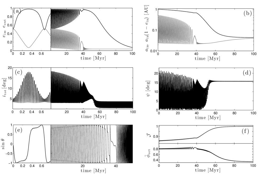
Figure 5.— Evolution of two planets initially in orbits (inner and outer) with $a_{\rm in}=1$ AU, $e_{\rm in}=0.51$, $a_{\rm out}=8$ AU, $e_{\rm out}=0.51$, and mutual inclination $i_{\rm tot}=5^{\circ}$. Initially the arguments of pericenter are $\omega_{\rm in}=\omega_{\rm out}=0$, the ascending nodes are $\Omega_{\rm in}=0$ and $\Omega_{\rm out}=180^{\circ}$, and the stellar obliquity is $\psi=0$ (angle between the stellar spin and angular momentum vector of the inner planet). The planets have masses of $m_{\rm in}=2M_{J}$ and $m_{\rm out}=3.3M_{J}$. We chose planetary and stellar viscous times of $t_{V,p}=0.03$ yr and $t_{V,s}=50$ yr, respectively (see text in §3). Panel (a): eccentricities of the inner ($e_{\rm in}$, black line) and outer ($e_{\rm out}$, gray line) planets. Panel (b): semi-major axis (black line) and pericenter distance $a_{\rm in}(1-e_{\rm in})$ (gray line) of the inner planet. Panel (c): mutual inclination between the two planetary orbits. Panel (d): stellar obliquity (angle between the host star’s spin axis and the orbital angular momentum vector of the inner orbit). Panel (e): $\sin\theta=\left(\bf{\hat{e}}_{\rm out}\times\bf{\hat{e}}_{\rm in}\right)\cdot\bf{\hat{h}}_{\rm in}$ (Eq. [23]). Note that the maximum time shown in this panel is $50$ Myr, as opposed to 100 Myr as in the other panels. Panel (f): dimensionless total orbital angular momentum $\mathcal{J}$ in Equation (3) (upper panel) and dimensionless interaction potential $\tilde{\phi}_{\rm oct}$ in Equation (LABEL:eq:potential) (lower panel).

3. Evolution during Migration

In Figure 5, we show an example of the secular evolution of two planets in initially eccentric ($e_{\rm in}=e_{\rm out}=0.51$) and low mutual inclination ($i_{\rm tot}=5^{\circ}$) orbits .

The equations of motion are fully described in Petrovich (2015a) (see appendix A therein), where the efficiency of tidal dissipation is parametrized by the viscous timescales of the star and the planet $t_{V,s}$ and $t_{V,p}$. For reference, a highly eccentric ($1-e\ll 1$) Jupiter-like planet orbiting a Solar-mass star with $a>1$ AU can be circularized to become a hot Jupiter with final $a=0.05$ AU ($a=0.06$ AU) within 1 Gyr for $t_{V,p}\lesssim 0.35$ yr ($t_{V,p}\lesssim 0.15$ yr) (Socrates et al., 2012). Given our choice of $t_{V,s}$ and $t_{V,p}$, tides in the planet dominate the circularization of the planetary orbit.

From panel a, we observe that the inner and outer planets efficiently exchange angular momentum: the inner orbit oscillates in eccentricity in the range $\simeq 0.48-0.97$, while the outer orbit does so in the range $\simeq 0.05-0.52$. These large-amplitude oscillations allow the inner planet to reach a minimum pericenter distance of $a_{\rm in}(1-e_{\rm in})\simeq 0.024$ AU where tidal dissipation can efficiently extract orbital energy (panel b). Thus, the orbit shrinks steadily during the phases in which the pericenter distances are small. From panel b, we observe that the semi-major axis decays almost linearly during the first $\sim 40$ Myr, after which the eccentricity oscillations are damped and the migration speeds up. The final semi-major axis of the HJ formed in this example is $\simeq 0.044$ AU, which roughly corresponds to the mean and median of $\simeq 0.05$ AU observed population of hot Jupiters detected in RV and transit surveys.

From panel c, we observe that the mutual inclination between the planetary orbits oscillates in the range $i_{\rm tot}\simeq 3-18^{\circ}$. The time at which $i_{\rm tot}$ reaches its maximum value of $\simeq 18^{\circ}$ coincides with the time at which $e_{\rm in}$ also reaches a maximum. However, the inclination shows many oscillations within one oscillation of the eccentricities because the former varies in the quadrupole timescale, while the latter does so in the octupole timescale (Li et al., 2014a). We note that in the coplanar limit ($i_{\rm tot}=0$), the quadrupole potential is axisymmetric (see first term in Equation [LABEL:eq:potential]), implying that it does not drive any angular momentum exchange between the orbits. However, if the orbits have non-zero (but still small) mutual inclinations, the quadrupole potential can still drive small amplitude eccentricity and inclination oscillations. Given the scale of panel c relative to that in panel a, the quadrupole-driven oscillations can only be observed in $i_{\rm tot}$ and their amplitude is modulated by the octupole potential.

Once the eccentricity oscillations are damped at $\sim 40$ Myr the inclination oscillations are no longer modulated by the octupole and vary only in the quadrupole timescale with decreasing amplitude. These oscillations change in character at $\gtrsim 50$ Myr, after which the mutual inclination damps to small values ($i_{\rm tot}\lesssim 3^{\circ}$) and oscillates due to the planetary orbital precession produced by the host star’s bulge. This flattening of the inner orbit has been previously observed by Correia et al. (2013) in a similar context of hierarchical two-planet systems.

From panel d we observe that the stellar obliquity (i.e., the angle between the host star’s spin axis and the orbital angular momentum vector of the inner orbit) starts oscillating in the range $\psi\simeq 0-20^{\circ}$ due to the perturbations of the outer planet. Once the planetary orbit starts flattening at $\gtrsim 50$ Myr, the conservation of angular momentum forces the obliquity to increase and it does so from $\sim 10^{\circ}$ to $\sim 20^{\circ}$. After $\gtrsim 60$ Myr the semi-major axis is $\lesssim 0.2$ AU and the planetary orbital precession is dominated by host star’s bulge rather than the outer planet. Thus, the stellar obliquity stabilizes at $\psi\simeq 16^{\circ}$.

In summary, our example ends with the formation of a hot Jupiter at $a\simeq 0.044$ AU with a stellar obliquity of $\psi\simeq 16^{\circ}$ and planetary perturber at 8 AU, which is in a circular and nearly coplanar orbit relative to the hot Jupiter.

3.1. Secular eccentricity forcing

The equations of motion of the eccentricity and angular momentum vectors can be obtained by taking gradients of the dimensionless potential (e.g., Tremaine et al. 2009; Petrovich 2015a). Evidently, from Equation (LABEL:eq:potential) $\nabla_{h_{\rm{in}}}\tilde{\phi}_{\rm oct}=0$ and the equation of motion of the eccentricity vector of the inner planet becomes

$$\frac{d{\bf e}_{\rm{in}}}{dt}=\frac{1}{\tau_{\rm in}}(1-e_{\rm{in}}^{2})^{1/2}{\bf\hat{h}}_{\rm{in}}\times\nabla_{e_{\rm{in}}}\tilde{\phi}_{\rm oct},$$ (20)

where

$$\tau_{\rm in}=\frac{2}{3\pi}\left(\frac{m_{1}}{m_{\rm out}}\right)\left(\frac{a_{\rm out}}{a_{\rm in}}\right)^{3}P_{\rm in}$$ (21)

and $P_{\rm in}$ is the orbital period of the inner planet. From this equation, we can calculate the eccentricity forcing term (i.e., the term proportional to ${\bf\hat{e}}_{\rm{in}}$ in Eq. [20]) as (see also Lee & Peale 2003; Li et al. 2014a)

$$\frac{de_{\rm in}}{dt}\simeq-\frac{5\alpha}{4\tau_{\rm in}}\frac{e_{\rm out}(1-e_{\rm in}^{2})^{1/2}(1+3e_{\rm in}^{2}/4)}{(1-e_{\rm out}^{2})^{5/2}}\sin\theta,$$ (22)

where we define

$$\sin\theta=\left(\bf{\hat{e}}_{\rm out}\times\bf{\hat{e}}_{\rm in}\right)\cdot\bf{\hat{h}}_{\rm in}.$$ (23)

Note that the angle $\theta$ coincides with $\varpi=\varpi_{\rm in}-\varpi_{\rm out}$ when the orbits are coplanar.

Similarly, one can differentiate ${\bf e}_{\rm in}\cdot{\bf e}_{\rm out}\equiv e_{\rm in}e_{\rm out}\cos\varpi$ to find

$$\frac{d\varpi}{dt} \simeq \frac{1}{\tau_{\rm in}}\bigg{\{}\frac{(1-e_{\rm in}^{2})^{1/2}}{(1-e_{\rm out}^{2})^{3/2}}-\mu\alpha^{1/2}\frac{(1+3e_{\rm in}^{2}/2)}{(1-e_{\rm out}^{2})^{2}}$$ (24)

$$-\frac{5\alpha}{4}\bigg{[}\frac{e_{\rm out}(1-e_{\rm in}^{2})^{1/2}(1+9e_{\rm in}^{2}/4)}{e_{\rm in}(1-e_{\rm out}^{2})^{5/2}}$$

$$-\mu\alpha^{1/2}\frac{e_{\rm in}(1+4e_{\rm out}^{2})(1+3e_{\rm in}^{2}/4)}{e_{\rm out}(1-e_{\rm out}^{2})^{3}}\bigg{]}\cos\varpi\bigg{\}}.$$

We note from Equations (22) and (24) that the planet masses change the timescale of the secular gravitational interactions through $\tau_{\rm in}$ and the evolution of $\varpi$ through $\mu$.

The timescale for the eccentricity growth is roughly $\tau_{\rm in}/\alpha$, which for our example in Figure 5 it corresponds to $\simeq 0.27$ Myr, consistent with the timescale of $\sim 0.3$ Myr that it takes for the eccentricity to grow from $\simeq 0.5$ to $\simeq 1$ (panel a).

In panel e of Figure 5, we show the evolution of $\sin\theta$ for the example. As expected from Equation (22), we observe that the eccentricity of the inner planet (panel a) increases (decreases) when $\sin\theta<0$ ($\sin\theta>0$).

In this simulation $\sin\theta$ starts at $0$ and rapidly decreases to $\simeq-1$ ($\theta\simeq 270^{\circ}$), where it remains oscillating close to this value. At some point, $\sin\theta$ jumps from $\simeq-1$ to $\simeq 1$ ($\theta\simeq 90^{\circ}$) and stays around this angle, while the eccentricity of the inner planet starts decreasing. This behavior is sketched in the energy levels of Figure 1 (black line in panel c), where we observe that the eccentricity growth (or decrease) happens mostly for $\varpi\sim 90^{\circ}$ (or $\sim 270^{\circ}$).

This behavior can be understood from Equation (22) where we observe that the slow variation of $\sin\theta$ around $\pm 1$ allows for a persistent eccentricity growth or decay. Moreover, from Equation (24) the slow variation of $\sin\theta$ around $\pm 1$ (i.e., $\cos\varpi\simeq 0$) happens when $e_{\rm in}$ and $e_{\rm out}$ are such that $\mu\alpha^{1/2}\simeq(1-e_{\rm in}^{2})^{1/2}(1-e_{\rm out}^{2})^{1/2}/(1+3e_{\rm in}^{2}/2)$, so $d\varpi/dt\simeq 0$ (Lee & Peale, 2003). This last condition implies that in the test particle approximation ($\mu\ll 1$), this resonant-like behavior can not happen unless $1-e_{\rm in}\ll 1$.

In summary, in this example we show that the eccentricity forcing can be enhanced by having a slow variation of $\varpi$ around $90^{\circ}$ or $270^{\circ}$, which can achieved for either not too small values of $\mu\alpha^{1/2}$ or high enough eccentricities.

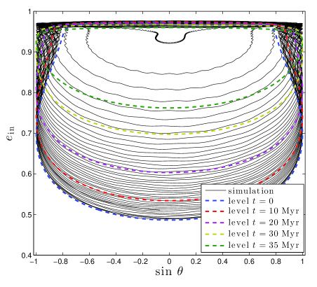
Figure 6.— Evolution of $\sin\theta$ and the inner eccentricity from the example in Figure 5 for the first 42.4 Myr of the simulation, at which time the oscillations are fully quenched. We also plot the contour levels of $\tilde{\phi}_{\rm extra}$ in Equation (19) using the values of $\alpha$, $\mathcal{J}$, and $\tilde{\phi}_{\rm extra}$ that correspond to different times of the example, as labeled.

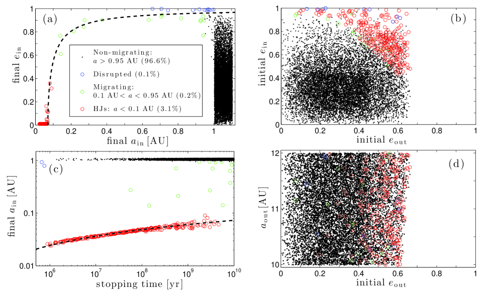
Figure 7.— Outcomes for our population synthesis study, as labeled in panel (a). We chose planetary and stellar viscous times of $t_{V,p}=0.1$ yr and $t_{V,s}=50$ yr, respectively (see text in §3). The inner planet has a mass of $1M_{J}$ and an initial semi-major axis drawn from a uniform distribution in [1,1.1] AU, while the outer planet has a mass uniformly distributed in $[1.3,1.7]M_{J}$ and an initial semi-major axis drawn from a uniform distribution in $[10,12]$ AU. The eccentricities of both the inner and outer planets are drawn from the distribution in Equation (25) with $\sigma_{e}=0.3$. Panel (a): final semi-major axis versus final eccentricity of the planetary orbit. The constant angular momentum track $a_{\rm in}(1-e_{\rm in}^{2})=0.07$ AU is indicated by a dashed line. Panel (b): initial eccentricity of the outer planet $e_{\rm out}$ versus the initial eccentricity of the inner planet $e_{\rm in}$. The boundary at high eccentricity reflects the stability condition for hierarchical triple systems given by Equation (26). Panel (c): time at which the simulation is stopped versus the final semi-major axis of the inner planet $a_{\rm in}$. The dashed line shows the empirical fit $\log\left(t_{\rm mig}/1{\rm Myr}\right)=0.82\times a_{\rm in}/0.01~{}{\rm AU}-2$, where $t_{\rm mig}$ is the timescale for the migration of the HJ with a final semi-major axis $a_{\rm in}$. Panel (d): initial eccentricity $e_{\rm out}$ versus the semi-major axis of the outer planet.

3.2. Quenching of the eccentricity oscillations

We observe from Figure 5 that as the semi-major axis shrinks (panel b), the eccentricity oscillations of the inner planet start to damp: the minimum value of $e_{\rm in}$ in each oscillation increases as a function of time. The oscillations are completely damped at $\simeq 42$ Myr.

We observe from panel e that the oscillatory behavior of $\sin\theta$ discussed in the previous section continues up to $\sim 30$ Myr and then the planet gradually starts spending less time at $\sin\theta\sim 1$, where the eccentricity forcing is maximum. Then, at $\sim 40$ Myr $\sin\theta$ stops librating and circulates in a timescale that is shorter than the octupole timescale.

In panel f we show the evolution of the dimensionless angular momentum $\mathcal{J}$ (Eq. [3]) and potential $\tilde{\phi}_{\rm oct}$ (Eq. [LABEL:eq:potential]).

First, we observe that $\mathcal{J}$ increases nearly monotonically from $\simeq 0.86$ to $1$ (i.e., to two nearly circular orbits). Second, $\tilde{\phi}_{\rm oct}$ stays roughly constant with small oscillations around $\simeq 0.83$ during the first $\sim 40$ Myr and then decreases monotonically to $\simeq 1/3$ (i.e., $e_{\rm in}=e_{\rm in}=0$ in Eq. [LABEL:eq:potential]).

In Figure 6 we show the evolution of $e_{\rm in}$ and $\sin\theta$ from our example. We show the results up to a maximum time of $42.4$ Myr, at which time the eccentricity oscillations are almost fully quenched and $\theta$ starts circulating. We also plot the phase-space trajectories from the energy contours of $\tilde{\phi}_{\rm extra}$ in Equation (19) and fixing $a_{\rm in}$, $\mathcal{J}$, and $\tilde{\phi}_{\rm extra}$ to match the simulation at different times. We observe that the phase-space trajectories roughly match the numerical example and describe well the quenching of the eccentricity oscillations. This result shows that the quenching of the eccentricity oscillations is mainly due to the monotonic increase of $\mathcal{J}$ in time.

Thus, this analysis suggests that in order to have eccentricity oscillations down to smaller $a_{\rm in}$ (or smaller $\alpha$) during migration, one might either need to start from smaller $\mathcal{J}$ or set $\mu$ to be smaller so $\mathcal{J}$ increases more slowly with the decreasing $\alpha$.

4. Population synthesis study

We ran a series of numerical experiments to study the evolution of triple systems consisting a sun-like host star ($m_{1}=1M_{\odot}$ and $R_{1}=R_{\odot}$) and two orbiting planets with masses $m_{\rm in}$ and $m_{\rm out}$. The inner planet has $m_{\rm in}=1M_{J}$ and Jupiter radius, while the outer has a mass that is randomly distributed in $[1.3,1.7]M_{J}$. This choice of masses is motivated by our results in §2.2, where we find that CHEM works best for outer planets slightly more massive than the inner planet. The equations of motion are fully described in Petrovich (2015a).

The initial eccentricity and mutual inclination of the planets follow a Rayleigh distribution:

$$dp=\frac{x\,dx}{\sigma_{x}^{2}}\exp\left(-\frac{1}{2}x^{2}/\sigma_{x}^{2}\right),$$ (25)

where $x=i,e$. We choose $\sigma_{e}=0.3$, which is intended to represent the tail ($e\gtrsim 0.3$) of the observed eccentricity distribution of giant planets ($m\sin i>0.1M_{J}$) with periods longer than 1 year. For the mutual inclinations we choose $\sigma_{i}=0.1$, or a mean of $\approx 7^{\circ}$, which is slightly higher than the upper limit to the mean mutual inclination of $\approx 5^{\circ}$ constrained from Kepler (Tremaine & Dong, 2012; Fabrycky et al., 2014).

The semi-major axis of the inner planet is drawn from a uniform distribution in $[1,1.1]$ AU, while that of the outer planet is drawn from a uniform distribution in $[10,12]$ AU. We discard systems that do not satisfy the stability condition (Mardling & Aarseth, 2001):

$$\frac{a_{\rm{out}}}{a_{\rm{in}}} > 2.8(1+\tilde{\mu})^{2/5}\frac{(1+e_{\rm out})^{2/5}}{(1-e_{\rm out})^{6/5}}\left(1-0.3\frac{i_{\rm tot}}{180^{\circ}}\right)$$ (26)

where $\tilde{\mu}=m_{\rm out}/(m_{1}+m_{\rm in})$.

The longitudes of the arguments of pericenter and longitude of the ascending node are chosen randomly for the inner and outer orbits. The host star and the planet start spinning with periods of 10 days and 10 hours, respectively, both along the ${\bf\hat{h}}_{\rm{in},0}$ axis, implying that the initial obliquities are zero.

Finally, we stop each run when a maximum time chosen uniformly in $[0,10]$ Gyr has passed or when either a hot Jupiter in a circular orbit ($e_{\rm in}<0.01$) is formed or a planet is tidally disrupted, which we define to occur when the pericenter distance is less than 0.0127 AU (Guillochon et al., 2011).

4.1. Results

In Figure 7, we show the results from our population synthesis study, which consists of 9,000 systems.

Most systems ($\simeq 96.6\%$, black dots) do not reach eccentricities that are high enough to allow for migration. In these systems, the mean eccentricity of the inner planet increases only slightly from an initial value of $\simeq 0.34$ to a final value of $\simeq 0.35$. Actually, the steady-state final eccentricity distribution looks essentially identical to the initial distribution, which means that by construction it can reproduce the observed eccentricity distribution of planets at $>1$ AU.

The second most common outcome ($\simeq 3.1\%$) is a system with a hot Jupiter ($a_{\rm in}<0.1$ AU, red circles). From panel b we observe that these systems initially have large eccentricities: the mean eccentricity of the inner and outer planets is 0.71 and 0.52, respectively. Note that the maximum eccentricity of the outer planet is $\simeq 0.66$, which is an artifact of the stability criterion in Equation (26) (see boundary at high $e_{{\rm out},i}$ in panel d of Figure 7). As discussed in §2, in order to form a hot Jupiter from an initial circular orbit we require a perturber with $e_{\rm out}>0.67$, which explains the lack of hot Jupiters that come from initial eccentricities $e_{\rm in}<0.4$. This restriction can be relaxed by using a less restrictive stability boundary for hierarchical triple systems like the ones proposed by Eggleton & Kiseleva (1995) and Petrovich (2015b).

The third most common outcome ($\simeq 0.2\%$) is a system with a migrating planet (0.1 AU $<a_{\rm in}<0.95$ AU, green circles). From panel a we observe that these systems have high eccentricities close to the angular momentum track $a_{\rm in}(1-e_{\rm in}^{2})=0.07$ AU.

Finally, the least common outcome ($\simeq 0.1\%$) is a system in which the inner planet gets tidally disrupted ($a_{\rm in}[1-e_{\rm in}]<0.0127$ AU at some point of the simulation, blue circles). Most of these systems start from very high eccentricities ($e_{\rm in}>0.99$) and crossed the tidal disruption boundary at the start of the simulation.

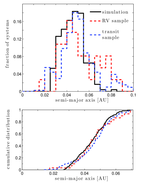
Figure 8.— Semi-major axis distribution of the hot Jupiters formed in our population synthesis study (solid line) and the observed distribution of planets with $m\sin i>0.1M_{J}$ detected in RV (red dashed line) and transit (blue dashed line) surveys. The transit sample is corrected for the geometric selection bias. The cumulative distribution in the lower panel is restricted to hot Jupiters with semi-major axis up to 0.07 AU.

4.2. Semi-major axis distribution of hot Jupiters

In Figure 8 we show the semi-major axis distribution for the hot Jupiters formed in our population synthesis study and the observations of hot Jupiters with $m\sin i>0.1M_{J}$ detected in the transit and RV surveys.

From the upper panel, we observe that the distribution of semi-major axis in the simulation roughly matches the peak of the observed distribution: the mean (median) in the simulation are $\simeq 0.045$ AU ($\simeq 0.045$ AU), while the observations have 0.052 AU (0.048 AU) and 0.050 AU (0.049 AU) in the RV and transit samples, respectively.

We note that the semi-major axis distribution drops for $a\lesssim 0.03$ AU, which is consistent with our analysis in §2.3 where we show that the minimum pericenter distance that this mechanism can achieve (for similar parameters) is $\simeq 0.015$ AU implying a minimum semi-major axis the HJs of $\simeq 0.03$ AU.

From panel a of Figure 4 we observe that for $\mu=m_{\rm in}/m_{\rm out}\in[0.58,0.77]$ (equivalent to $m_{\rm out}=[1.3,1.7]M_{J}$ as in the synthesis study) and $e_{\rm in}=0.6$ the maximum eccentricities in the range $0.95-0.985$ and the exact value increases with the initial eccentricity of the outer planet $e_{\rm out}$. Since the simulation starts with $e_{\rm out}$ taken from a Rayleigh distribution (Eq. [25]), then it is more likely for the inner planet to reach lower maximum eccentricities and larger pericenter distances in this range and, therefore, the HJs would tend to have higher semi-major axes. This result qualitatively explains why the semi-major axis distribution in the simulation does not peak at the smallest allowed values.

From Figure 8 we observe that our numerical study mostly forms HJs with $a_{\rm in}<0.07$ AU, while $\sim 7\%$ and $\sim 19\%$ of the observed HJs have $a_{\rm in}>0.07$ AU in transit and RV surveys, respectively. From the lower panel we observe that by restricting our sample to HJs with $a<0.07$ AU, our population study describes the observed distribution fairly well ($p-$values $\gtrsim 0.1$).

The observed population of HJs with $a>0.07$ AU can be explained by CHEM by increasing the efficiency of tidal dissipation, which might be achieved by either decreasing the planetary viscous time $t_{V,p}$ or considering an initially inflated planet as in Petrovich (2015a).

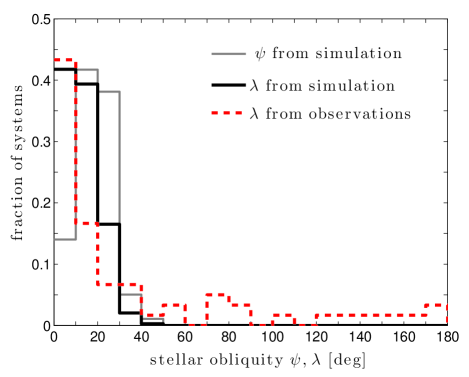
Figure 9.— Distribution of the stellar obliquity $\psi$ (gray solid line) and sky-projected stellar obliquity $\lambda$ (black solid line) of the hot Jupiters formed our population synthesis study. The sample of 60 hot Jupiters with $m\sin i>0.1M_{J}$ and projected obliquity measurements is shown in red dashed line.

4.3. Obliquity distribution of hot Jupiters

As of September 2014, the observed sample of hot Jupiters (planets with $M\sin(i)>0.1M_{J}$ and $a<0.1$ AU) contains 60 planets with projected stellar obliquity measurements $\lambda$ with mean and median of $\simeq 38^{\circ}$ and $\simeq 14^{\circ}$.

In Figure 9 we show the distribution of obliquities $\psi$ and projected obliquities $\lambda$ from our population synthesis study and compare this with the observed data. From our simulations we measure the angle between the spin axis of the host star and the normal of the inner planetary orbit $\psi$ (often called the stellar obliquity angle or misalignment angle). We then calculate $\lambda$, the sky-projected value of $\psi$, by taking $10^{5}$ random orbital configurations relative to a fixed observer for each system (see e.g., Fabrycky & Winn 2009).

We observe that the final distribution of $\psi$ is concentrated towards $10^{\circ}-30^{\circ}$, while the HJ systems initially have zero obliquity and a low mutual inclination $i_{\rm tot}$ (mean and median of $\sim 7^{\circ}$). Similar to our example in Figure 5 the moderate excitation of $\psi$ comes from the excitation of $i_{\rm tot}$ during the high-eccentricity phases of the system’s evolution. Thus, the range of $\psi$ in HJ systems formed by CHEM depends on range of the initial mutual inclination. We checked this conclusion by considering initially flatter systems (lower values of $i_{\rm tot}$), and indeed found that the distribution of $\psi$ shifts to lower values.

In Figure 9 we observe that our population synthesis study of CHEM produces HJs with $\lambda<40^{\circ}$ and typically ($\sim 80\%$) $\lambda<20^{\circ}$. This result compares favorably with the data because most planets ($\sim 60\%$) in the observations have $\lambda<20^{\circ}$. However, CHEM fails to explain the systems with $\lambda>40^{\circ}$, which correspond to $\sim 25\%$ of the observed sample.

These systems with higher obliquities must be produced by another mechanism such as the Kozai-Lidov mechanism in stellar binaries (e.g., Wu & Murray 2003; Fabrycky & Tremaine 2007; Naoz et al. 2012; Petrovich 2015a), planet-planet scattering (e.g., Nagasawa et al. 2008; Nagasawa & Ida 2011; Beaugé & Nesvorný 2012), or other secular interactions between planets (e.g., Naoz et al. 2011; Wu & Lithwick 2011). The higher obliquities can also be due to a primordial misalignment of the proto-planetary disk relative to the host star’s spin axis (e.g., Bate et al. 2010; Lai et al. 2011; Batygin 2012; Crida & Batygin 2014; Spalding & Batygin 2014) or a tilt of the outer layers of the host stars (Rogers et al., 2012; Rogers & Lin, 2013).

We note that any primordial alignment of the stellar spin axis from the proto-planetary disk in which the proto-hot Jupiter is ultimately formed would be nearly preserved for the planetary orbit undergoing CHEM. This property has been previously attributed to the hot Jupiters formed through disk-driven migration since these planets remain in the same plane as a the proto-planetary disk during migration. Our simulations show that high-eccentricity migration can also preserve the alignment between the stellar spin and planetary orbits.

4.4. Migration timescale of hot Jupiters

From panel c in Figure 7 we observe that the migration timescale $t_{\rm mig}$ (or stopping time in the simulation) of hot Jupiters in circular orbits (red circles) increases monotonically with the final semi-major axis $a_{\rm in}$.

We show that the empirical expression $\log\left(t_{\rm mig}/1{\rm Myr}\right)=0.82\times a_{\rm in}/0.01~{}{\rm AU}-2$ (black dashed line) gives a good fit to the to the migration timescale as a function of the final semi-major axis $a_{\rm in}$. This expression is only valid for the parameters used in our population synthesis study: a Jupiter-like planet ($R_{\rm in}=1R_{J}$, $m_{\rm in}=1M_{J}$) with a viscous time of the planet $t_{V,p}=0.1$ yr orbiting a Sun-like star ($R_{\rm 1}=1R_{\odot}$, $m_{\rm 1}=1M_{\odot}$). From Petrovich (2015a) (Equation 10 therein) we have that the migration timescale depends on these parameters as $t_{\rm mig}\propto t_{V,p}\left(m_{\rm in}/m_{1}\right)^{2}R_{\rm in}^{-8}$, implying that the migration timescale can be written as

$$\log\left(t_{\rm mig}/1{\rm Myr}\right) = 0.82\times\frac{a_{\rm in}}{0.01~{}{\rm AU}}+\log\left(\frac{t_{V,p}}{0.1~{}{\rm yr}}\right)$$

$$+ 2\log\left(\frac{m_{\rm in}}{m_{1}}\frac{M_{\odot}}{M_{J}}\right)-8\log\left(\frac{R_{\rm in}}{R_{J}}\right)-2.$$

This timescale can be used to compare this migration scenario with observations: a HJ with a given semi-major axis $a$ should be older than $t_{\rm mig}$ from our fit. For instance, Quinn et al. (2012) recently discovered two HJs in the 600 Myr Beehive cluster, with current semi-major axes 0.032 AU and 0.052 AU. Our empirical formula gives a minimum migration timescale of $\sim 4$ Myr and $\sim 180$ Myr, respectively. Thus, the migration timescales predicted by our population synthesis study of CHEM are both within the age of the cluster.

Finally, we note that we stop the simulation when the HJ reaches an eccentricity $e<0.01$, while the subsequent tidal dissipation in the star can change the semi-major axis of the planet, specially for short-period ($<3$ days) planets. However, most stars hosting HJs have rotation periods longer than $\sim 3$ days and, therefore, tides in the star are expected to shrink the semi-major axis of these short-period planets, making our constraint of the minimum timescale still valid.

4.5. Outer planets in hot Jupiter systems

The outer planets in our simulated hot Jupiter systems initially have moderately high eccentricities (mean and median of 0.53 and 0.54), while at the end of the simulations they have somewhat lower eccentricities (mean and median of 0.32 and 0.33). This reduction in the eccentricity of the outer planet is expected because HJs are only formed when they lose almost all their angular momentum, which is mostly transferred to the orbit of the outer planet.

We expect that the outer planets with larger semi-major axes and larger masses are less affected by this reduction in eccentricity because they have higher initial angular momentum and, therefore, can retain larger final eccentricities. In particular, we observe a strong positive correlation (coefficient of $\simeq 0.54$) between $e_{\rm out}$ and $a_{\rm out}$ in our simulations.

The outer planets in HJ systems have an initial mean mutual inclination of $\simeq 7.7^{\circ}$, which decreases slightly to $\simeq 6^{\circ}$ once the HJ is formed.

We have restricted our population synthesis study to a limited range in semi-major axes and masses of the outer body because the parameter space is large and the initial conditions are fairly uncertain. We can, however, place constraints on these parameters based on our analytical calculations in §§2.2.1 and 2.2.2, where we show in Equations (10) and (13) that CHEM operates with the minimum eccentricity of the outer planet for

$$m_{\rm out}a_{\rm out}^{1/2}=\tilde{C}\times m_{\rm in}a_{\rm in}^{1/2},$$ (28)

where $\tilde{C}\simeq 3.3$ and $\tilde{C}\simeq 6.2$ for an initial inner planet with zero eccentricity and with eccentricity equal to that of the outer planet, respectively. The approximation that CHEM mostly operates with the minimum eccentricity of the outer planet is justified if its distribution decreases rapidly for $e_{\rm out}\gtrsim 0.5$, as is observed in the sample of giant planets at $a>1$ AU.

On the other hand, the dynamical stability of the system requires that $a_{\rm out}/a_{\rm in}\gtrsim 8$ and $a_{\rm out}/a_{\rm in}\gtrsim 5$ for an initial inner planet with zero eccentricity and with eccentricity equal to that of the outer planet, respectively from these initial conditions, respectively. Note that by increasing $a_{\rm out}/a_{\rm in}$ CHEM becomes less efficient since both the GR and the tidal quadrupole strongly limit the eccentricity growth (see Eqs. [15] and [17]) and CHEM requires higher outer eccentricities to operate (see Figure 2). Thus, the most likely initial semi-major axis ratios are probably close to $a_{\rm out}/a_{\rm in}\sim 5-8$.

Roughly speaking, from the arguments above we conclude that if the inner planet commenced CHEM at $a_{\rm in}\sim 1$ AU, the most likely properties of outer planet are $a_{\rm out}\sim 5-8$ AU and $m_{\rm out}/m_{\rm in}\sim 1-3$ (from Eq. [28]).

In summary, the outer planets in HJ systems formed by CHEM have moderate eccentricities ($e_{\rm out}\sim 0.2-0.5$) and low mutual inclinations relative to the HJ’s orbit. Their eccentricities are expected to be larger for outer perturbers at wider separations or with higher masses. Based on the minimum initial eccentricities required for CHEM to operate we determine the most likely semi-major axis and mass ratios to be $a_{\rm out}/a_{\rm in}\sim 5-8$ and $m_{\rm out}/m_{\rm in}\sim 1-3$, respectively.

5. Discussion

5.1. Comparison with previous work

5.1.1 Retrograde vs prograde HJs from CHEM

We have shown that CHEM produces hot Jupiters in prograde and low obliquity orbits (assuming an initially zero misalignment of the planetary orbit relative to host star spin). On the contrary, Li et al. (2014a) concluded that CHEM is a mechanism to produce counter-orbiting hot Jupiters (obliquities of $\sim 180^{\circ}$).

We understand this difference from the necessary condition to flip the orbit from prograde to retrograde, which is that eccentricity forcing mechanism studied here can produce extremely high eccentricities: $1-e_{\rm in}\lesssim 10^{-3}-10^{-4}$ (Li et al., 2014a). In order for this to happen the migrating planet has to be initially placed at large enough semi-major axis to satisfy the following requirements:

• the planet does not get tidally disrupted by reaching pericenter that are too close to the host star. For instance, according to Guillochon et al. (2011) a Jupiter-like planet orbiting a sun-like star gets disrupted if $a_{\rm in}(1-e_{\rm in})\lesssim 0.013$ AU, which implies that that the planet should start at $a_{\rm in}\gtrsim 13$ AU to avoid disruption when $1-e_{\rm in}\lesssim 10^{-3}$.

• extra precession forces (e.g., GR precession) do not efficiently limit the eccentricity growth. As discussed in §2.3, the maximum eccentricity depends on $a_{\rm in}$ as $1-e_{\rm in,max}\propto a_{\rm in}^{-2}$ ($1-e_{\rm in,max}\propto a_{\rm in}^{-10/9}$) if the dominant precession source is GR (the tidal quadrupole). Thus, all other things being equal, the maximum eccentricity can reach higher values for larger semi-major axes.

In this work, we have considered an initial semi-major axes in $a_{\rm in}=1-5$ AU and the effects from GR precession, tides, and tidal disruptions. Therefore, the maximum eccentricity is not high to allow for orbit flipping (see maximum eccentricities in Figure 4), although it does allow for moderate excitation (up to $\sim 20^{\circ}$) of the mutual inclination between the orbits (see panel c in Figure 5).

In the systematic study of coplanar flips by Li et al. (2014a), the authors ignore the effects from tides and tidal disruptions, and consider the test particle limit $\mu\ll 1$ for which the extra precession forces like GR become much less efficient than the planetary regime considered here ($\mu\sim 1$) at limiting the maximum eccentricity growth. Recall from the arguments in §2.3 that $1-e_{\rm in,max}\propto\mu^{2}$ if GR is the dominant precession force. All these approximations allow for the inner eccentricity to reach extremely high values and flip. The authors do consider the effect of tides and tidal disruptions in one example of an orbit flip (Figure 7 therein), but in this example the inner planet is initially placed at large enough distances ($a_{\rm in}\sim 40$ AU) that it can avoid both being tidally disrupted and having the eccentricity growth efficiently limited by extra precession forces.

In summary, CHEM generally produces hot Jupiters with low obliquities. It might, however, produce highly mis-aligned hot Jupiters provided that the migrating planet starts migration from a large ($\gg 1$ AU) semi-major axis.

5.1.2 Other secular high-eccentricity migration scenarios

Various high-eccentricity migration mechanisms have been shown to produce hot Jupiters from gravitational interactions between planets like in CHEM. We briefly comment on the main differences between these mechanisms and CHEM.

First, hot Jupiters can be formed by the chaotic secular interactions between two or more planets in eccentric and/or mutually inclined orbits, proposed and termed secular chaos by Wu & Lithwick (2011). Here, the eccentricity excitation is chaotic and depends on the mutual inclination between planets since coplanar systems become much more regular. On the contrary, the eccentricity excitation from CHEM is regular (non-chaotic) and does not depend on the initial mutual inclination provided that it is not too high ($\gtrsim 20^{\circ}$). Both CHEM and secular chaos predict that hot Jupiters should have distant planetary companions. CHEM requires of only one companion, while secular chaos does favor having two or more planetary companions because the system has more degrees of freedom.

Second, hot Jupiters might be formed by the Kozai-Lidov (KL) mechanism (Naoz et al., 2011, 2012; Petrovich, 2015a). Unlike CHEM, the KL mechanism would require that the planetary orbits have initially high ($\gtrsim 50^{\circ}$) mutual inclinations (e.g., Teyssandier et al. 2013). Also the eccentricity excitation in CHEM happens in the octupole timescale that is longer by a factor of $\sim a_{\rm out}/a_{\rm in}$ than the quadrupole timescale that governs the KL mechanism. This slower eccentricity excitation allows for extra precession forces such as GR and tides to limit the maximum eccentricity growth more efficiently, leading to the formation of hot Jupiters with semi-major axes generally larger than those expected from KL migration.

All the mechanisms above, including CHEM, require an initial configuration with well-spaced and eccentric or/and mutually inclined orbits either of additional planets or stellar companions. Given that we do not know the initial states of planetary systems, it is difficult to assess which mechanism is more likely to be prevalent. One natural candidate to explain the initial conditions required for these different high-eccentricity migration scenarios is planet-planet scattering starting from initially unstable planetary systems (e.g., Jurić & Tremaine 2008; Chatterjee et al. 2008). We plan to address which set of initial conditions are more likely to emerge from scattering in a future work (Petrovich & Tremaine 2015, in prep.)

5.2. Summary of predictions by CHEM

We have shown that CHEM can produce hot Jupiters. Whether CHEM produces most hot Jupiters is a more difficult issue to address since we do not know the initial states of planetary systems. However, we can partly address this issue by comparing the predictions from CHEM with the available (or upcoming) observations.

Coplanar High-eccentricity Migration predicts:

1. a pile-up of hot Jupiters at $a\sim 0.04-0.05$ AU.

   This pile-up is a natural consequence from CHEM since it excites the eccentricity of the migrating planet very slowly (slower than the Kozai-Lidov mechanism by a factor $\sim a_{\rm out}/a_{\rm in}$) allowing for pericenter precession forces due to general relativity and tides to efficiently limit the maximum eccentricity growth (see Figure 4). This limit in the eccentricity translates into a minimum pericenter distance and the formation of a hot Jupiter with semi-major axis roughly twice this minimum distance, as discussed in §4.2.

   This predicted concentration of hot Jupiters with $a\sim 0.04-0.05$ AU compares well with the observations of hot Jupiters detected in transit and RV surveys (see Figure 8).

2. hot Jupiters with low stellar obliquities.

   The low stellar obliquities of HJ systems are a natural consequence of CHEM since the eccentricity of the migrating planet can be excited to high values without exciting its inclination. This result shows that, like disk-driven migration, high-eccentricity migration can also preserve the alignment between the stellar spin and planetary orbits.

   Our population synthesis study shows that CHEM mostly produces HJs with projected obliquities $\lesssim 30^{\circ}$, and almost $70\%$ of the current observations fall into this range. The remaining population of mis-aligned hot Jupiters might be explained by either another high-eccentricity migration channel or a mechanism that tilts the star or the plane of the planetary system.

3. a few percent occurrence rate of hot Jupiters per distant giant planet.

   Our population synthesis study shows that $\sim 3\%$ of the systems produce a hot Jupiter. This number mostly depends on the initial eccentricities since most HJs are formed starting from $e_{\rm in}>0.5$ and $e_{\rm out}\sim 0.4-0.7$, a range containing $\sim 15\%$ and $\sim 20\%$ of the known planets with $a>1$ AU, respectively. This fraction can increase by:

   • shifting the stability boundary for hierarchical triple systems (Eq. [26]) towards higher eccentricities. Indeed, we repeated the population synthesis study using the less restrictive stability condition $a_{\rm out}(1-e_{\rm out})>1.7a_{\rm in}(1+e_{\rm in})$ from Eggleton & Kiseleva (1995) and observed that the occurrence rate increased from $3.1\%$ in our study using Equation (26) to $5.2\%$;

   • starting with positively correlated inner and outer eccentricities, which might be expected from an initial scattering phase.

   If CHEM dominates the formation of HJs then the ratio between the number of HJs and the number of gas giant planets should be $\sim 3-5\%$. This ratio is roughly consistent with the one derived from observations of $\sim 3-10\%$ since the occurrence rate of HJs is $\sim 0.5-1.5\%$ (Gould et al., 2006; Mayor et al., 2011) and that of the gas giant planet at AU distances is $\sim 15\%$ (Mayor et al., 2011).

4. hot Jupiters have distant massive companions in nearly coplanar and moderately eccentric orbits.

   The most likely outer planets in HJ systems formed by CHEM have moderate eccentricities ($e_{\rm out}\sim 0.2-0.5$), low inclinations ($<10^{\circ}$) relative to the HJ’s orbit, and masses $\sim 1-3$ times larger than that of the HJ (see §4.5). Also, the most likely semi-major axis ratio before commencing migration is $a_{\rm out}/a_{\rm in}\sim 5-8$ so assuming that CHEM started at $a>1$ AU, we expect companions at $a\gtrsim 5$ AU.

   Since the RV surveys have characterized giant planets with full orbits up to $a\sim 5$ AU, we expect that most of the companions predicted by CHEM generally appear as RV linear trends. Recently, Knutson et al. (2014) estimated that $51\%\pm 10\%$ of the HJs have a companion with $a_{\rm out}=1-20$ AU and masses of $m_{\rm out}=1-13M_{J}$, while the masses of the planetary companion tend to be comparable to or larger than the transiting HJs. This range of planetary masses and semi-major axes is consistent with CHEM.

   There are three systems with hot Jupiters and an outer companion with eccentricity and semi-major axis measurements:

   • HD 217107 contains a HJ at 0.075 AU with $e\simeq 0.12$ and $m\sin i\simeq 1.41M_{J}$, and a companion at 6.07 AU with $e\simeq 0.38$ and $m\sin i\simeq 4.5M_{J}$ (Vogt et al., 2005; Feng et al., 2015),

   • HD 187123 contains a HJ at 0.042 AU in a circular orbit with $m\sin i\simeq 0.51M_{J}$ and a companion at $\simeq 4.4$ AU with $e\simeq 0.28$ and $m\sin i\simeq 1.8M_{J}$ (Vogt et al., 2005; Wright et al., 2009; Feng et al., 2015),

   • HAT-P-13 contains a HJ at 0.043 AU in a circular orbit with $m\simeq 0.85M_{J}$ and a companion at 1.22 AU with $e\simeq 0.66$ and $m\sin i\simeq 14M_{J}$ (Bakos et al., 2009). The hot Jupiter has a projected obliquity of $\lambda=1.9^{\circ}\pm 8.6^{\circ}$ (Winn et al., 2010).

   We observe that the eccentricities and mass ratios (assuming nearly coplanar orbits) from HD 217107 and HD 187123 are roughly consistent with the most likely range predicted from CHEM of $e\sim 0.2-0.5$ and $\sim 1-3$, respectively. This result suggests that CHEM might have operated to form these close-in planets. Migration in these systems should have commenced within $\sim 1$ AU since the companions are at $a\sim 5$ AU.

   On the contrary, HAT-P-13 has a mass ratio $>17$ and the perturber is at $\sim 1$ AU, making CHEM an unlikely formation scenario. Moreover, given the high eccentricity of the outer planet the stability boundary of hierarchical triple systems in Equation (26) constrains the inner planet to $a\lesssim 0.1$ AU and, therefore, inconsistent with any high-eccentricity migration scenario.

5. HJ formation timescales that increase exponentially with semi-major axis.

   From our population synthesis study we find that the minimum timescale to form a hot Jupiter depends exponentially with semi-major and found an empirical fit given by Equation (4.4). As discussed in §4.4, this minimum formation timescale for the two hot Jupiters in the Beehive cluster is consistent with its age 600 Myr (Quinn et al., 2012). Future age constraints from hot Jupiter systems might prove useful to constrain CHEM.

   More generally speaking, this minimum formation timescale from CHEM implies that the occurrence rate of hot Jupiters should increase with stellar age and that the hot Jupiters with larger semi-major axes should be restricted to older systems. The former observation is consistent with the difference between the HJ abundances in Kepler and RV surveys (e.g., Dawson & Murray-Clay 2013).

6. a population of eccentric and low-obliquity close-in planets

   Depending on the age of the planetary system and the efficiency of tidal dissipation, CHEM is expected to produce planets which have experienced significant orbital migration, but have not had enough time to become a HJ in a circular orbit (see planets with final $e_{\rm in}>0.4$ and $a_{\rm in}<0.3$ AU in Figure 7). These planets are eccentric and have relatively low stellar obliquities ($\psi\lesssim 20^{\circ}$).

   There are three planetary systems with a giant planet with $a<0.3$ AU, eccentricity of $e>0.4$, and with a measurement of its projected stellar obliquity $\lambda$:

   • HD 17156 b is a planet with mass $\simeq 3.3M_{J}$ at $a=0.16$ AU with eccentricity $e\simeq 0.68$, and projected obliquity $\lambda=10^{\circ}\pm 5^{\circ}$ (Fischer et al., 2007; Narita et al., 2009),

   • HAT-P-2 b is a planet with mass $8.9\pm 0.4M_{J}$ at $a=0.068$ AU with eccentricity $e\simeq 0.52$, and projected obliquity $\lambda=10^{\circ}\pm 5^{\circ}$ (Bakos et al., 2007; Albrecht et al., 2012),

   • HAT-P-34 b is a planet with mass $3.3\pm 0.2M_{J}$ at $a=0.068$ AU with eccentricity $e\simeq 0.44$, and projected obliquity $\lambda=0^{\circ}\pm 14^{\circ}$ (Bakos et al., 2012; Albrecht et al., 2012).

   We observe that all these three planets in close-in and eccentric orbits have low projected obliquities ($\lambda\lesssim 10^{\circ}$), suggesting that CHEM might have operated to form these systems. This observation is particularly interesting because these planets are hardly produced by other migration mechanism. Other high-eccentricity migration mechanisms can produce high-eccentricity close-in planets similar to CHEM, but these planets generally have higher obliquities (e.g., Fabrycky & Tremaine 2007; Beaugé & Nesvorný 2012). Similarly, disk-migration can naturally produce low-obliquity close-in planets, but neither disk-migration (e.g., Kley & Nelson 2012) nor planet-planet scattering after migration to small orbital separations are expected to excite high eccentricities (Johansen et al., 2012; Petrovich et al., 2014).

6. Conclusions

We study the secular gravitational interaction of two planets in a hierarchical configuration with relatively low mutual inclinations and eccentric orbits, including the effects from general relativity, tides, and stellar rotation.

We show that the eccentricity of the inner planet can be excited to very high values starting from: an inner planet in a circular orbit and an outer planet with eccentricity of $\gtrsim 0.67$ or two eccentric orbits ($e\gtrsim 0.5$). The excitation is most efficient (i.e., requires the smallest initial eccentricities) when the semi-major axis ratio $\alpha=a_{\rm in}/a_{\rm out}$ and mass ratio $\mu=m_{\rm in}/m_{\rm out}$ are in the following range $\mu(\alpha/0.1)^{1/2}\sim 0.5-0.8$.

We show that this mechanism, which we term Coplanar High-eccentricity Migration (CHEM) can preserve the alignment between the stellar spin and the planetary orbits, generally forming hot Jupiters with low stellar obliquities. Based on a population synthesis study we show the hot Jupiters produced by CHEM can well-reproduce the observed semi-major axis distribution of hot Jupiters and can account for their observed occurrence rates.

We predict that the hot Jupiters formed by CHEM should have distant ($\gtrsim 5$ AU) planetary companions in low mutual inclination and moderately eccentric ($e\sim 0.2-0.5$) orbits and with most likely masses $\sim 1-3$ times larger than that of the HJ.

References

- Albrecht et al. (2012) Albrecht, S., Winn, J. N., Johnson, J. A., et al. 2012, ApJ, 757, 18
- Bakos et al. (2007) Bakos, G. Á., Kovács, G., Torres, G. et al. 2007, ApJ, 670, 826
- Bakos et al. (2009) Bakos, G. Á., Howard, A. W., Noyes, R. W., et al. 2009, ApJ, 707, 446
- Bakos et al. (2012) Bakos, G. Á ., Hartman, J. D., Torres, G., et al. 2012, AJ, 144, 19
- Bate et al. (2010) Bate, M. R., Lodato, G., & Pringle, J. E. 2010, MNRAS, 410, 1505
- Batygin (2012) Batygin, K. 2012, Natur, 491, 418
- Beaugé & Nesvorný (2012) Beaugé, C., & Nesvorný, D. 2012, ApJ, 751, 119
- Bodenheimer et al. (2000) Bodenheimer, P., Hubickyj, O., & Lissauer, J. J. 2000, Icar, 143, 2
- Chambers (1999) Chambers, J. E. 1999, MNRAS, 304, 793
- Chatterjee et al. (2008) Chatterjee, S., Ford, E. B., Matsumura, S., & Rasio, F. A. 2008, ApJ, 686, 580
- Correia et al. (2013) Correia, A.C.M, Boué, G., Laskar, J., & Morais, M.H.M. 2013, A&A, 553, A39
- Crida & Batygin (2014) Crida, A., & Batygin, K. 2014, A&A, 567, A42
- Dawson & Murray-Clay (2013) Dawson, R., & Murray-Clay, R. A. 2013, ApJL, 767, L24
- Dawson et al. (2014) Dawson, R. I., Johnson, J. A.; Fabrycky, D. C, et al. 2014, ApJ, 791, 89
- Eggleton & Kiseleva (1995) Eggleton, P., & Kiseleva, L. 1995, ApJ, 455, 640
- Eggleton et al. (1998) Eggleton, P. P., Kiseleva, L. G., & Hut, P. 1998, ApJ, 499, 853
- Fabrycky et al. (2014) Fabrycky, D. C., Lissauer, J. J., Ragozzine, D., et al. 2014, ApJ, 790, 146
- Fabrycky & Tremaine (2007) Fabrycky, D., & Tremaine, S. 2007, ApJ, 669, 1298
- Fabrycky & Winn (2009) Fabrycky, D., & Winn, J. 2009, ApJ, 696, 1230
- Ford & Rasio (2008) Ford, E. B., & Rasio, F. A. 2008, ApJ, 686, 621
- Feng et al. (2015) Feng, Y. K., Wright, J. T., Nelson, B. et al 2015, arXiv:1501.00633
- Fischer et al. (2007) Fischer, D. A., Vogt, S. S., Marcy, G. W., et al. 2007, ApJ, 669, 1336
- Goldreich & Tremaine (1980) Goldreich, P., & Tremaine, S. 1980, ApJ, 241, 425
- Gould et al. (2006) Gould, A., Dorsher, S., Gaudi, B. S., & Udalski, A. 2006, Acta Astron., 56, 1
- Guillochon et al. (2011) Guillochon, J., Ramirez-Ruiz, E., & Lin, D. 2011, ApJ, 732, 74
- Hellier et al. (2012) Hellier, C., Anderson, D. R., Collier Cameron, A., et al. 2012, MNRAS, 426, 739
- Howard et al. (2012) Howard, A. W., Marcy, G. W., Bryson, S. T., et al. 2012, ApJS, 201, 15
- Johansen et al. (2012) Johansen, A., Davies, M. B., Church, R. P., & Holmelin, V. 2012, ApJ, 758, 39
- Jurić & Tremaine (2008) Jurić, M., & Tremaine, S. 2008, ApJ, 686, 603
- Kane & Raymond (2014) Kane, S. R., & Raymond, S. N. 2014, ApJ, 784, 104
- Kley & Nelson (2012) Kley, W., & Nelson, R. P. 2012, AARA, 50, 211
- Knutson et al. (2014) Knutson, H. A., Fulton, B. J., Montet, B. T., et al. 2014, ApJ, 785, 126
- Lai et al. (2011) Lai, D., Foucart, F., & Lin, D. N. C. 2011, MNRAS, 412, 2790
- Lee & Peale (2003) Lee, M. H., & Peale, S. J. 2003, ApJ, 592, 1201
- Li et al. (2014a) Li, G., Naoz, S., Kocsis, B., & Loeb, A. 2014a, ApJ, 785, 116
- Li et al. (2014b) Li, G., Naoz, S., Holman, M., & Loeb, A. 2014b, ApJ, 791, 86
- Lin & Ida (1997) Lin, D. N. C. & Ida, S. 1997, ApJ, 477, 781
- Libert & Henrard (2005) Libert, A.-S., & Henrard, J. 2005, Celest. Mech. Dyn. Astron., 93, 187
- Liu et al. (2014) Liu, B.; Muñoz, D. J.; Lai, D. 2015, MNRAS, 447, 1
- Malhotra (2002) Malhotra, R. 2002, ApJL, 575, L33
- Marcy et al. (2005) Marcy, G., Butler, R. P., Fischer, D., et al. 2005, Prog. Theor. Phys. Suppl., 158, 24
- Mardling & Aarseth (2001) Mardling, R. A., & Aarseth, S. J. 2001, MNRAS, 321, 398
- Mayor et al. (2011) Mayor, M., et al. 2011, arXiv:1109.2497
- Michtchenko & Malhotra (2004) Michtchenko, T. A., & Malhotra, R. 2004, Icarus, 168, 237
- Michtchenko et al. (2006) Michtchenko, T. A., Ferraz-Mello, S., & Beaugé, C. 2006, Icarus, 181, 555
- Migaszewski & Goździewski (2009) Migaszewski, C., & Goździewski, K. 2009, MNRAS, 395, 1777
- Nagasawa et al. (2008) Nagasawa, M., Ida, S., & Bessho, T. 2008, ApJ, 678, 1
- Nagasawa & Ida (2011) Nagasawa, M., & Ida, S. 2011, ApJ742, 72
- Naoz et al. (2011) Naoz, S., Farr, W. M., Lithwick, Y., Rasio, F. A., & Teyssandier, J. 2011, Natur, 473, 187
- Naoz et al. (2012) Naoz, S., Farr, W. M., & Rasio, F. A. 2012, ApJ, 754, L36
- Narita et al. (2009) Narita N. et al., 2009, PASJ, 61, 991
- Petrovich et al. (2014) Petrovich, C., Tremaine, S., & Rafikov, R. 2014, ApJ, 782, 101
- Petrovich (2015a) Petrovich, C. 2015a, ApJ, 799, 27
- Petrovich (2015b) Petrovich, C. 2015b, arXiv:1506.05464
- Quinn et al. (2012) Quinn, S. N., White, R. J., Latham, D. W., et al. 2012, ApJ, 756, L33
- Rasio & Ford (1996) Rasio, F. A., & Ford, E. B. 1996, Science, 274, 954
- Rogers et al. (2012) Rogers, T. M., Lin, D. N. C., & Lau, H. H. B. 2012, ApJ, 758, L6
- Rogers & Lin (2013) Rogers, T. M., & Lin, D. N. C. 2013, ApJ, 769, L10
- Socrates et al. (2012) Socrates, A., Katz, B., & Dong, S. 2012, arXiv:1209.5724
- Spalding & Batygin (2014) Spalding, C., & Batygin, K. 2014, ApJ, 790, 42
- Teyssandier et al. (2013) Teyssandier, J., Naoz, S., Lizarraga, I., & Rasio 2013, ApJ, 779, 166
- Timpe et al. (2013) Timpe, M., Barnes, R., Kopparapu, R., et al. 2013, ApJ, 146, 63
- Tremaine & Dong (2012) Tremaine, S., & Dong, S. 2012, AJ, 143, 94
- Tremaine et al. (2009) Tremaine, S., Touma, J., & Namouni, F. 2009, AJ, 137, 3706
- Vogt et al. (2005) Vogt, S. S., Butler, R. P., Marcy, G. W., et al. 2005, ApJ, 632, 638
- Ward (1997) Ward, W. R. 1997, Icar, 126, 261
- Weidenschilling & Marzari (1996) Weidenschilling, S. J. & Marzari, F., 1996, Natur, 384, 619
- Winn et al. (2010) Winn, J. N., Johnson, J. A., Howard, A. W., et al. 2010, ApJ, 718, 575
- Wright et al. (2009) Wright, J. T., Upadhyay, S., Marcy, G. W., et al. 2009, ApJ, 693, 1084
- Wright et al. (2011) Wright J. T. et al. 2011, PASP, 123, 412
- Wright et al. (2012) Wright, J. T., Marcy, G. W., Howard, A. W., et al. 2012, ApJ, 753, 160
- Wu & Lithwick (2011) Wu, Y. & Lithwick, Y. 2011, ApJ, 735,109
- Wu & Murray (2003) Wu, Y. & Murray, N. 2003, ApJ, 589, 605