Convergence of statistical moments of particle density time series in scrape-off layer plasmas

Abstract

Particle density fluctuations in the scrape-off layer of magnetically confined plasmas, as measured by gas-puff imaging or Langmuir probes, are modeled as the realization of a stochastic process in which a superposition of pulses with a fixed shape, an exponential distribution of waiting times and amplitudes represents the radial motion of blob-like structures. With an analytic formulation of the process at hand, we derive expressions for the mean squared error on estimators of sample mean and sample variance as a function of sample length, sampling frequency, and the parameters of the stochastic process. Employing that the probability distribution function of a particularly relevant stochastic process is given by the gamma distribution, we derive estimators for sample skewness and kurtosis, and expressions for the mean squared error on these estimators. Numerically generated synthetic time series are used to verify the proposed estimators, the sample length dependency of their mean squared errors, and their performance. We find that estimators for sample skewness and kurtosis based on the gamma distribution are more precise and more accurate than common estimators based on the method of moments.

I Introduction

Turbulent transport in the edge of magnetically confined plasmas is a key issue to be understood on the way to improved plasma confinement, and ultimately commercially viable fusion power. Within the last-closed magnetic flux surface, time series of the particle density present small relative fluctuation amplitudes and Gaussian amplitude statistics. The picture in the scrape-off layer (SOL) is quite different. Time series of the particle density, as obtained by single point measurements, present a relative fluctuation level of order unity. Sample coefficients of skewness and excess kurtosis foot-1 of these time series are non vanishing and sample histograms feature elevated tails. This implies that the deviation from normality is caused by the frequent occurrence of large amplitude events LABEL:antar-2001,_antar-2003,_xu-2005,_agostini-2007,_dewhurst-2008.

These features of fluctuations in the scrape-off layer are attributed to the radially outwards motion of large amplitude plasma filaments, or blobs. Time series of the plasma particle density obtained experimentally LABEL:boedo-2003,_agostini-2007,_xu-2009,_tanaka-2009,_cheng-2010,_nold-2010 and by numerical simulations LABEL:russell-2007,_garcia-2007-tcv,_russell-2007,_myra-2008,_militello-2012 show that estimated coefficients of skewness and excess kurtosis LABEL:balanda-1988 increase radially outwards with distance to the last closed flux surface. At the same time one observes a parabolic relationship between these two coefficients and that the coefficient of skewness vanishes close to the last closed flux surface LABEL:russell-2007,_graves-2005,_sattin-2006,_labit-2007,_cheng-2010,_garcia-2013.

Recently, it was proposed to model the observed particle density time series by a shot noise process LABEL:rice-1977, that is, a random superposition of pulses corresponding to blob structures propagating through the scrape-off layer LABEL:garcia-2012. Describing individual pulses by an exponentially decaying waveform with exponentially distributed pulse amplitudes and waiting time between consecutive pulses leads to a Gamma distribution for the particle density amplitudes LABEL:garcia-2012,_garcia-2006-tcv. In this model, the shape and scale parameter of the resulting Gamma distribution can be expressed by the pulse duration time and average pulse waiting time.

In order to compare predictions from this stochastic model to experimental measurements, long time series are needed, as to calculate statistical averages with high accuracy. Due to a finite correlation time of the fluctuations, an increased sampling frequency may increase the number of statistically independent samples only up to a certain fraction. Then, only an increase in the length of the time series may increase the number of independent samples. This poses a problem for Langmuir probes, which are subject to large heat fluxes and may therefore only be dwelled in the scrape-off layer for a limited amount of time. Optical diagnostics on the other hand, may observe for an extended time interval but have other drawbacks, as for example the need to inject a neutral gas into the plasma to increase the signal to noise ratio, and that the signal intensity depends sensitively on the plasma parameters LABEL:zweben-2002,_stotler-2003,_cziegler-phd.

This work builds on the stochastic model presented in Ref. LABEL:garcia-2012 by proposing estimators for the mean, variance, skewness and excess kurtosis of a shot noise process and deriving expressions of their mean squared error as a function of sample length, sampling frequency, pulse amplitude, and duration, and waiting time. Subsequently, we generate synthetic time series of the shot noise process at hand. The mean squared error of the proposed estimators is computed of these time series and their dependence on the sampling parameters and the process parameters is discussed.

This paper is organized as follows. Section II introduces the stochastic process that models particle density fluctuations and the correlation function of this process. In Section III we propose statistical estimators to be used for the shot-noise process and derive expressions for the mean squared error on these estimators. A comparison of the introduced estimators and expressions for their mean squared error to results from analysis of synthetic time series of a shot noise process is given in Section IV. A summary and conclusions are given in Section V.

II Stochastic model

A stochastic process formed by superposing the realization of independent random events is commonly called a shot noise process LABEL:rice-1977,_pecseli-book-fluct. Denoting the pulse form as $\psi(t)$, the amplitude as $A_{k}$, and the arrival time as $t_{k}$, a realization of a shot noise process with $K$ pulses is written as

$$\Phi_{K}(t) =\sum\limits_{k=1}^{K}A_{k}\psi(t-t_{k}).$$ (1)

To model particle density time series in the scrape-off layer by a stochastic process, the salient features of experimental measurements have to be reproduced by it.

Analysis of experimental measurement data from tokamak plasmas, LABEL:antar-2003,_dewhurst-2008,_xu-2005,_boedo-2003,_cheng-2010,_garcia-2007-tcv,_garcia-2006-tcv as well as numerical simulations LABEL:garcia-2006-tcv,_bian-2003,_garcia-2006,_kube-2011, have revealed large amplitude bursts with an asymmetric wave form, featuring a fast rise time and a slow exponential decay. The burst duration is found to be independent of the burst amplitude and the plasma parameters in the scrape-off layer LABEL:garcia-2009,_garcia-2013. The waveform to be used in Eq. (1) is thus modeled as

$$\psi_{k}(t)=\exp\left(-\frac{t}{\tau_{\mathrm{d}}}\right)\Theta(t),$$ (2)

where $\tau_{\mathrm{d}}$ is the pulse duration time and $\Theta$ denotes the Heaviside step function. Analysis of long data time series further reveals that the pulse amplitudes $A$ are exponentially distributed LABEL:garcia-2013,

$$P_{A}(A)=\frac{1}{\langle A\rangle}\exp\left(-\frac{A}{\langle A\rangle}\right).$$ (3)

Here $\langle A\rangle$ is the scale parameter of the exponential distribution, and $\langle\cdot\rangle$ denotes an ensemble average. The waiting times between consecutive bursts are found to be exponentially distributed LABEL:antar-2001,_antar-2003,_garcia-2013,_furchert-2013. Postulating uniformly distributed pulse arrival times $t$ on an interval length $T$, $P_{t}(t)=1/T$, it follows that the total number of pulses in a fixed time interval, $K$, is Poisson distributed and that the waiting time between consecutive pulses, $\tau_{\mathrm{w}}$, is therefore also exponentially distributed LABEL:pecseli-book-fluct.

Under these assumptions it was shown that the stationary amplitude distribution of the stochastic process given by Eq. (1) is a Gamma distribution LABEL:garcia-2012,

$$P_{\Phi}(\Phi) =\frac{1}{\Gamma(\gamma)}\left(\frac{\gamma}{\langle\Phi\rangle}\right)^{\gamma}\Phi^{\gamma-1}\exp\left(-\frac{\gamma\Phi}{\langle\Phi\rangle}\right),$$ (4)

with the shape parameter given by the ratio of pulse duration time to the average pulse waiting time

$$\gamma=\frac{\tau_{\mathrm{d}}}{\tau_{\mathrm{w}}}.$$ (5)

This ratio describes the intermittency of the shot noise process. In the limit $\gamma\ll 1$, individual pulses appear isolated whereas $\gamma\gg 1$ describes the case of strong pulse overlap. In Ref. LABEL:garcia-2012 it was further shown that the mean, $\langle\Phi\rangle$, the variance, $\text{var}\left(\Phi\right)=\langle\left(\Phi-\langle\Phi\rangle\right)^{2}\rangle$, the coefficient of skewness, $S\left(\Phi\right)$, and the coefficient of flatness, or excess kurtosis, $F\left(\Phi\right)$, are in this case given by

$$\langle\Phi\rangle =\langle A\rangle\frac{\tau_{\mathrm{d}}}{\tau_{\mathrm{w}}}, \text{var}\left(\Phi\right) =\langle A\rangle^{2}\frac{\tau_{\mathrm{d}}}{\tau_{\mathrm{w}}},$$ (6a)

$$S\left(\Phi\right) =2\left(\frac{\tau_{\mathrm{w}}}{\tau_{\mathrm{d}}}\right)^{1/2}, F\left(\Phi\right) =6\frac{\tau_{\mathrm{w}}}{\tau_{\mathrm{d}}}.$$ (6b)

Thus, the parameters of the shot noise process, $\tau_{\mathrm{d}}/\tau_{\mathrm{w}}$, and $\langle A\rangle$, may be estimated from the two lowest order moments of a time series. Before we proceed in the next section to define estimators for these quantities, we continue by deriving an expression for the correlation function of the signal given by Eq. (1). Formally, we follow the method outlined in Ref. LABEL:pecseli-book-fluct.

Given the definition of a correlation function, we average over the pulse arrival time and amplitude distribution and use that for an exponentially distributed pulse amplitude, $\langle A^{n}\rangle=n!\langle A\rangle$ holds. This gives

$$\langle\Phi_{K}(t)\Phi_{K}(t+\tau)\rangle =\int\limits_{0}^{T}\mathrm{d}t_{1}P_{t}(t_{1})\int\limits_{0}^{\infty}\mathrm{d}A_{1}P_{A}(A_{1})\cdots\int\limits_{0}^{T}\mathrm{d}t_{K}P_{t}(t_{K})\int\limits_{0}^{\infty}\mathrm{d}A_{K}P_{A}(A_{K})\times$$

$$\hskip 17.22217pt\sum\limits_{p=1}^{K}\sum\limits_{q=1}^{K}A_{p}\psi(t-t_{p})\,A_{q}\psi(t+\tau-t_{q})$$

$$=\langle A^{2}\rangle\sum\limits_{p=1}^{K}\int\limits_{0}^{T}\frac{\mathrm{d}t_{p}}{T}\psi(t-t_{p})\psi(t+\tau-t_{p})$$

$$+\langle A\rangle^{2}\sum\limits_{p\neq q}\int\limits_{0}^{T}\frac{\mathrm{d}t_{p}}{T}\int\limits_{0}^{T}\frac{\mathrm{d}t_{q}}{T}\psi(t-t_{p})\psi(t+\tau-t_{q}).$$ (7)

Here, we have divided the sum in two parts. The first part consists of $K$ terms where $p=q$ and the second part consists of $K(K-1)$ terms where $p\neq q$. The integral over a single pulse is given by

$$\int\limits_{0}^{T}\mathrm{d}t_{p}\;P_{t}(t_{p})\psi(t-t_{p})=\frac{\tau_{\mathrm{d}}}{T}\left[1-\exp\left(-\frac{t}{\tau_{\mathrm{d}}}\right)\right],$$ (8)

where the boundary term $\exp(-t/\tau_{\mathrm{d}})$ arises due to the finite integration domain. For observation times $t\gg\tau_{\mathrm{d}}$ this term vanishes and in the following we neglect it by ignoring the initial transient part of the time series where only few pulses contribute to the amplitude of the signal.

Within the same approximation, the integral of the product of two independent pulses is given by

$$\int\limits_{0}^{T}\mathrm{d}t_{p}\;P(t_{p})\psi(t-t_{p})\psi(t+\tau-t_{p})=\frac{\tau_{\mathrm{d}}}{2T}\exp\left(-\frac{|\tau|}{\tau_{\mathrm{d}}}\right).$$

Substituting these two results into Eq. (7), we average over the number of pulses occurring in $[0:T]$. Using that the total number of pulses is Poisson distributed and that the average waiting time between consecutive pulses is given by $\tau_{\mathrm{w}}=T/\langle K\rangle$, we evaluate the two-point correlation function of Eq. (1) as

$$\langle\Phi(t)\Phi(t+\tau)\rangle =\langle A\rangle^{2}\frac{\tau_{\mathrm{d}}}{\tau_{\mathrm{w}}}\left[\exp\left(-\frac{|\tau|}{\tau_{\mathrm{d}}}\right)+\frac{\tau_{\mathrm{d}}}{\tau_{\mathrm{w}}}\right].$$ (9)

Comparing this expression to the ensemble average of the model at hand, Eq. (6a), we find $\langle\Phi(t)\Phi(t+\tau)\rangle=\langle\Phi(t)\rangle\left[\langle A\rangle\exp\left(-|\tau|/\tau_{\mathrm{d}}\right)+\langle\Phi(t)\rangle\right].$ For $\tau\rightarrow\infty$, the correlation function decays exponentially to the square of the ensemble average.

III Statistical estimators for the Gamma distribution

The Gamma distribution is a continuous probability distribution with a shape parameter $\gamma$ and a scale parameter $\theta$. The probability distribution function (PDF) of a gamma distributed random variable $X>0$ is given by

$$P_{X}(X;\gamma,\theta) =\frac{X^{\gamma-1}}{\theta^{\gamma}\Gamma(\gamma)}\exp\left(-\frac{X}{\theta}\right),$$ (10)

where $\Gamma(x)=\int\limits_{0}^{\infty}\mathrm{d}u\,u^{x-1}e^{-u}$ denotes the gamma function. Statistics of a random variable are often described in terms of the moments of its distribution function, which are defined as

$$m_{k}=\int\limits_{0}^{\infty}\mathrm{d}X\;P_{X}(X;\gamma,\theta)x^{k},$$

and centered moments of its distribution function, defined as

$$\mu_{k}=\int\limits_{0}^{\infty}\mathrm{d}X\;\left[P_{X}(X;\gamma,\theta)-m_{1}\right]^{k}.$$

Common statistics used to describe a random variable are the mean $\mu=m_{1}$, the variance $\sigma^{2}=\mu_{2}$, skewness $S=\mu_{3}/\mu_{2}^{3/2}$ and excess kurtosis, or flatness, $F=\mu_{4}/\mu_{2}^{2}-3$. Skewness and excess kurtosis are well established measures to characterize asymmetry and elevated tails of a probability distribution function. For a Gamma distribution, the moments relate to the shape and scale parameter as

$$m_{1}=\gamma\theta,\qquad\mu_{2}=\gamma\theta^{2},\qquad\mu_{3}=2\gamma\theta^{3},\qquad\mu_{4}=6\gamma\theta^{4},$$

and coefficients of skewness and excess kurtosis are given in terms of the shape parameter by

$$S=\frac{\mu_{3}}{\mu_{2}^{3/2}}=\frac{2}{\sqrt{\gamma}},\qquad\qquad F=\frac{\mu_{4}}{\mu_{2}^{2}}-3=\frac{6}{\gamma}.$$

For the process described by Eq. (1), $\gamma$ is given by the ratio of pulse duration time to pulse waiting time, so that skewness and excess kurtosis assume large values in the case of strong intermittency, that is, weak pulse overlap.

In practice, a realization of a shot noise process, given by Eq. (1), is typically sampled for a finite time $T$ at a constant sampling rate $1/\triangle_{t}$ as to obtain a total of $N=T/\triangle_{t}$ samples. When a sample of the process is taken after the initial transient, where only few pulses contribute to the amplitude, the probability distribution function of the sampled amplitudes is given by the stationary distribution function of the process described by Eq. (4).

We wish to estimate the moments of the distribution function underlying a set of $N$ data points, $\{x_{i}\}_{i=1}^{N}$, which are now taken to be samples of a continuous shot noise process, obtained at discrete sampling times $t_{i}=i\cdot\triangle_{t}$, $x_{i}=\Phi(t_{i})$. Using the method of moments, estimators of mean, variance, skewness, and excess kurtosis are defined as

$$\widehat{\mu} =\frac{1}{N}\sum\limits_{i=1}^{N}x_{i}, \widehat{\sigma^{2}} =\frac{1}{N-1}\sum\limits_{i=1}^{N}\left(x_{i}-\widehat{\mu}\right)^{2},$$ (11a)

$$\widehat{S} =\frac{\sum\limits_{i=1}^{N}\left(x_{i}-\widehat{\mu}\right)^{3}}{\left(\sum\limits_{i=1}^{N}\left(x_{i}-\widehat{\mu}\right)^{2}\right)^{3/2}}, \widehat{F} =\frac{\sum\limits_{i=1}^{N}\left(x_{i}-\widehat{\mu}\right)^{4}}{\left(\sum\limits_{i=1}^{N}\left(x_{i}-\widehat{\mu}\right)^{2}\right)^{2}}-3.$$ (11b)

Here, and in the following, hatted quantities denote an estimator. Building on these, we further define an estimator for the intermittency parameter of the shot noise process according to Eq. (6a)

$$\widehat{\gamma} =\frac{\widehat{\mu}^{2}}{\widehat{\sigma^{2}}}.$$ (12)

We use this estimator to define alternative estimators for skewness and excess kurtosis as

$$\widehat{S}_{\Gamma} =\frac{2}{\sqrt{\widehat{\gamma}}}, \widehat{F}_{\Gamma} =\frac{6}{\widehat{\gamma}}.$$ (13)

in accordance with Eq. (6b).

In general, any estimator $\widehat{U}$ is a function of $N$ random variables and therefore a random variable itself. A desired property of any estimator is that with increasing argument sample size its value converges to the true value that one wishes to estimate. The notion of distance to the true value is commonly measured by the mean squared error on the estimator $\widehat{U}$, given by

$$\mathrm{MSE}(\widehat{U})=\text{var}(\widehat{U})+\mathrm{bias}(\widehat{U},U)^{2},$$ (14)

where $\text{var}(\widehat{U})=\langle(\widehat{U}-\langle\widehat{U}\rangle)^{2}\rangle$, $\mathrm{bias}(\widehat{U},U)=\langle\langle\widehat{U}\rangle-U\rangle$, and $\langle\cdot\rangle$ denotes the ensemble average. When Eq. (11a) is applied to a sample of $N$ normally distributed and uncorrelated random variables, it can be shown that $\mathrm{bias}(\widehat{\mu},\mu)=0$, $\mathrm{bias}(\widehat{\sigma^{2}},\sigma^{2})=0$, and that the mean squared error of both estimators is inversely proportional to the sample size, $\mathrm{MSE}(\widehat{\mu})\sim N^{-1}$, and $\mathrm{MSE}(\widehat{\sigma^{2}})\sim N^{-1}$. For a sample of gamma distributed and independent random variables, $\langle\widehat{\mu}\rangle=\mu=\gamma\theta$ and $\langle\widehat{\sigma^{2}}\rangle=\mu_{2}=\gamma\theta^{2}$ holds. Thus the estimators defined in Eq. (11a) have vanishing bias and their mean-square error is given by their respective variance, $\text{var}(\widehat{\mu})$ and $\text{var}(\widehat{\sigma^{2}})$.

With $\gamma=\mu^{2}/\sigma^{2}$, the mean squared error on the estimators for sample mean and variance, given in Eq. (11a), can be propagated on to a mean-square error on Eq. (13) using Gaussian propagation of uncertainty:

$$\mathrm{MSE}(\widehat{S}_{\Gamma}) =4\frac{\widehat{\sigma^{2}}}{\widehat{\mu}^{4}}\mathrm{MSE}(\widehat{\mu})+\frac{1}{\widehat{\sigma^{2}}\widehat{\mu}^{2}}\mathrm{MSE}(\widehat{\sigma^{2}})-4\frac{1}{\widehat{\mu}^{3}}\mathrm{COV}(\widehat{\mu},\widehat{\sigma^{2}}),$$ (15)

$$\mathrm{MSE}(\widehat{F}_{\Gamma}) =144\frac{\widehat{\sigma^{2}}^{2}}{\widehat{\mu}^{6}}\mathrm{MSE}(\widehat{\mu})+36\frac{1}{\widehat{\mu}^{4}}\mathrm{MSE}(\widehat{\sigma^{2}})-144\frac{\widehat{\sigma^{2}}}{\widehat{\mu}^{5}}\mathrm{COV}(\widehat{\mu},\widehat{\sigma^{2}}).$$ (16)

Here $\mathrm{COV}(\widehat{A},\widehat{B})=\langle(\widehat{A}-\langle A\rangle)(\widehat{B}-\langle B\rangle)\rangle$. Thus, the mean squared errors on estimators for coefficients of skewness and excess kurtosis can be expressed through the mean squared errors on the mean and variance, and through the covariance between $\widehat{\mu}$ and $\widehat{\sigma^{2}}$.

We now proceed to derive analytic expressions for $\mathrm{MSE}(\widehat{\mu})$ and $\mathrm{MSE}(\widehat{\sigma^{2}})$. With the definition of $\widehat{\mu}$ in Eq. (11a), and using $\langle\widehat{\mu}\rangle=\mu=\langle\Phi(t)\rangle$, we find

$$\mathrm{MSE}(\widehat{\mu})=\langle\left(\widehat{\mu}-\mu\right)^{2}\rangle=-\langle\Phi(t)\rangle^{2}+\frac{1}{N^{2}}\sum\limits_{i=1}^{N}\sum\limits_{j=1}^{N}\langle\Phi(t_{i})\Phi(t_{j})\rangle.$$ (17)

In order to evaluate the sum over the discrete correlation function, we evaluate the continuous two-point correlation function given by Eq. (9) at the discrete sampling times, with a discrete time lag given by $\tau=\tau_{ij}=t_{i}-t_{j}$. This gives

$$\mathrm{MSE}(\widehat{\mu}) =\frac{1}{N}\langle A\rangle^{2}\frac{\tau_{\mathrm{d}}}{\tau_{\mathrm{w}}}\left[1+\frac{1}{N}\sum\limits_{\begin{subarray}{c}i,j=1\\ i\neq j\end{subarray}}^{N}\exp\left(-\frac{|\tau_{ij}|}{\tau_{\mathrm{d}}}\right)\right].$$

Defining $\alpha=\triangle_{t}/\tau_{\mathrm{d}}$, we evaluate the sum as a geometric series,

$$\frac{1}{2}\sum\limits_{\begin{subarray}{c}i,j=1\\ i\neq j\end{subarray}}^{N}\exp\left(-\frac{|\tau_{ij}|}{\tau_{\mathrm{d}}}\right) =\frac{N+e^{-\alpha N}-1-Ne^{-\alpha}}{2\sinh^{2}\left(\alpha/2\right)},$$ (18)

to find the mean squared error

$$\mathrm{MSE}(\widehat{\mu}) =\frac{1}{N}\langle A\rangle^{2}\frac{\tau_{\mathrm{d}}}{\tau_{\mathrm{w}}}\left[1+\frac{1}{N}\frac{N+e^{-\alpha N}-1-Ne^{-\alpha}}{2\sinh^{2}\left(\alpha/2\right)}\right].$$ (19)

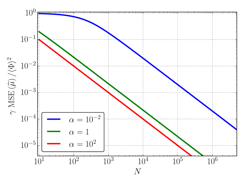
Figure 1: Relative mean squared error on $\widehat{\mu}$, given by Eq. (19), as a function of the number of data points $N$ for three values of the normalized sampling rate $\alpha=\triangle_{t}/\tau_{\mathrm{d}}$.

Fig. 1 shows the normalized mean squared error as a function of the of sample size, $N$. The parameter $\alpha$ relates the sampling time to the pulse duration time. For $\alpha\gg 1$, the obtained samples are uncorrelated, while the limit $\alpha\ll 1$ describes the case of high sampling frequency where the time series is well resolved on the time scale of the individual pulses. We find for the corresponding limits

$$\mathrm{MSE}(\widehat{\mu})=\frac{1}{N}\langle\Phi(t)\rangle^{2}\frac{\tau_{\mathrm{w}}}{\tau_{\mathrm{d}}}\times\begin{cases}1\quad&\alpha\gg 1,\\ 1+\frac{2}{N}\frac{e^{-\alpha N}-\left(1-\alpha N\right)}{\alpha^{2}}\quad&\alpha\ll 1.\end{cases}$$ (20)

For both limits, $\mathrm{MSE}(\widehat{\mu})$ is proportional to $\mu^{2}$ and inversely proportional to the intermittency parameter $\gamma=\tau_{\mathrm{d}}/\tau_{\mathrm{w}}$.

In the case of low sampling frequency, $\alpha\gg 1$, the mean squared error on the estimator of the mean becomes independent of the sampling frequency and is only determined by the parameters of the underlying shot noise process. In this case, the relative error $\mathrm{MSE}(\widehat{\mu})/\langle\Phi\rangle^{2}$ is inversely proportional to $\gamma$ and the number of data points $N$. Thus, a highly intermittent process, $\gamma\ll 1$, features a larger relative error on the mean than a process with significant pulse overlap, $\gamma\gg 1$. In the case of high sampling frequency, $\alpha\ll 1$, finite correlation effects contribute to the mean squared error on $\widehat{\mu}$, given by the non-canceling terms of the series expansion of $\exp(-\alpha N)$ in Eq. (20). Continuing with the high sampling frequency limit, we now further take the limit $\alpha N\gg 1$. This describes the case of a total sample time long compared to the pulse duration time, $T=N\triangle_{t}\gg\tau_{\mathrm{d}}$. In this case the mean square error on the mean is given by

$$\mathrm{MSE}(\widehat{\mu})=\frac{2}{\alpha N}\langle\Phi(t)\rangle^{2}\;\frac{\tau_{\mathrm{w}}}{\tau_{\mathrm{d}}}.$$ (21)

As in the low sampling frequency limit, the mean square error on $\mu$ converges as $N^{-1}$, but is larger by a factor of $2/\alpha$, where $\alpha$ was assumed to be small.

In Fig. 1 we present $\mathrm{MSE}(\widehat{\mu})\,$ for $\alpha=10^{-2}$, $1$, and $10^{2}$. The first value corresponds to the fast sampling limit, the second value corresponds to sampling on a time scale comparable to the decay time of an individual pulse and the third value corresponds to sampling on a slower time scale. The relative error for the case $\alpha\ll 1$ is clearly largest. For $N\lesssim 10^{4}$, the $N$ dependency of $\mathrm{MSE}(\widehat{\mu})$ is weaker than $N^{-1}$. Increasing $N$ to $N\gtrsim 10^{4}$ gives $\alpha N\gg 1$, such that $\mathrm{MSE}(\widehat{\mu})\sim 1/N$ holds. For $\alpha=1$, and $\alpha=10$, $\alpha N\gg 1$ holds, and we find that the relative mean squared error on the mean is inversely proportional to the number of samples $N$, in accordance with Eq. (20).

We note here, that instead of evaluating the geometrical sum that leads to Eq. (18) explicitly, it is more convenient to rewrite the sum over the correlation function in Eq. (17) as a Riemann sum and approximate it as an integral:

$$\sum\limits_{i\neq j}e^{-\alpha|i-j|}\simeq\int\limits_{0}^{N}\mathrm{d}i\;\int\limits_{0}^{N}\mathrm{d}j\left[\Theta(i-j)e^{\alpha(j-i)}+\Theta(j-i)e^{\alpha(i-j)}\right]=2\frac{\alpha N+e^{-\alpha N}-1}{\alpha^{2}}.$$ (22)

For the approximation to be valid, it is required that $\mathrm{d}i/N,\mathrm{d}j/N\ll 1$, and that the variation of the integrand over $\triangle_{i}\times\triangle_{j}$ must be small, $\alpha\ll 1$. Approximating the sum as in Eq. (22) therefore yields the same result for $\mathrm{MSE}(\widehat{\mu})$ as the limit $\alpha\gg 1$ given in Eq. (20).

Expressions for the mean squared error on the estimator $\widehat{\sigma^{2}}$ and the covariance $\mathrm{COV}(\widehat{\mu},\widehat{\sigma^{2}})$ are derived using the same approach as used to derive Eq. (19). With $\mathrm{MSE}(\widehat{\sigma^{2}})=\langle(\widehat{\sigma^{2}}-\sigma^{2})^{2}\rangle$, and $\mathrm{COV}(\widehat{\mu},\widehat{\sigma^{2}})=\langle(\widehat{\mu}-\mu)(\widehat{\sigma^{2}}-\sigma^{2})\rangle$, it follows from Eq. (11a) that expressions for summations over third and fourth order correlation functions of the signal given by Eq. (1) have to be evaluated to obtain closed expressions. Postponing the details of these calculations to the appendix, we present here only the resulting expressions. The mean squared error on the variance is given by

$$\mathrm{MSE}(\widehat{\sigma^{2}})=\langle A\rangle^{4}\left[\left(\frac{\tau_{\mathrm{d}}}{\tau_{\mathrm{w}}}\right)^{2}\left(\frac{2}{\alpha N}+\frac{-5-8e^{-\alpha N}+e^{-2\alpha N}}{\alpha^{2}N^{2}}\right)\right.$$

$$\left.\quad+\frac{\tau_{\mathrm{d}}}{\tau_{\mathrm{w}}}\left(\frac{6}{\alpha N}+\frac{-27+3e^{-2\alpha N}}{\alpha^{2}N^{2}}\right)\right]\quad+\mathcal{O}\left(N^{-3}\right),$$ (23)

while the covariance between the estimators of the mean and variance is given by

$$\mathrm{COV}(\widehat{\mu},\widehat{\sigma^{2}})=\langle A\rangle^{3}\left[\left(\frac{\tau_{\mathrm{d}}}{\tau_{\mathrm{w}}}\right)^{2}4\frac{1-e^{-\alpha N}}{\alpha^{2}N^{2}}+\frac{\tau_{\mathrm{d}}}{\tau_{\mathrm{w}}}\left(\frac{3}{\alpha N}+\frac{-17+4e^{-\alpha N}-4e^{-2\alpha N}}{2\alpha^{2}N^{2}}\right.\right.$$

$$\left.\left.+\frac{9-12e^{-\alpha N}+3e^{-2\alpha N}}{\alpha^{3}N^{3}}\right)\right].$$ (24)

The results, given in Eqs. (19), (23), and (24), are finally used to evaluate Eqs. (15), and (16), yielding the mean squared error on $\widehat{S}_{\Gamma}$ and $\widehat{F}_{\Gamma}$. The higher order terms in Eq. (23) are readily calculated by the method described in appendix A and are not written out here due to space restrictions.

In the limit $\alpha N\gg 1$, leading order terms in Eqs. (23) and (24) are inversely proportional to $\alpha N$:

$$\mathrm{COV}(\widehat{\mu},\widehat{\sigma^{2}}) =\frac{3}{\alpha N}\langle\Phi(t)\rangle\text{var}\left(\Phi(t)\right)\frac{\tau_{\mathrm{w}}}{\tau_{\mathrm{d}}}$$ (25)

$$\mathrm{MSE}(\widehat{\sigma^{2}}) =\frac{2}{\alpha N}\text{var}\left(\Phi(t)\right)^{2}\left(1+3\frac{\tau_{\mathrm{w}}}{\tau_{\mathrm{d}}}\right).$$ (26)

While Eqs. (21) and (25) are proportional to $\gamma$, $\mathrm{MSE}(\widehat{\sigma^{2}})$ depends also quadratically on $\gamma$.

IV Comparison to synthetic time series

In this section we compare the derived expressions for the mean squared error on the estimators for the sample mean, variance, skewness, and kurtosis, against sample variances from the respective estimators computed of synthetic time series of the stochastic process given by Eq. (1).

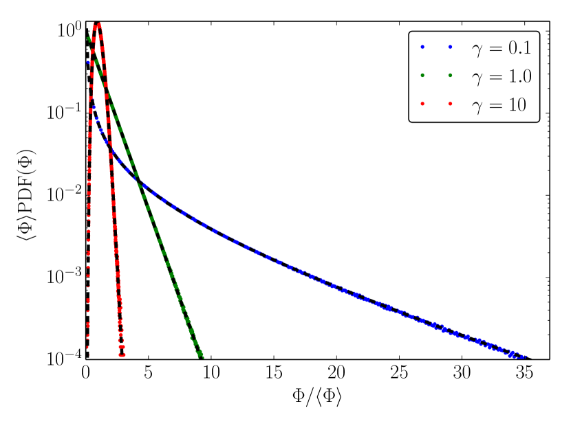
Figure 2: Histogram of synthetic time series with $\gamma=0.1$, $1.0$, and $10$. Overlaid (black dashed lines) is the Gamma distribution given by Eq. (4) with a scale parameter $\theta=1$.

To generate synthetic time series, the number of pulses $K$, the pulse duration time $\tau_{\mathrm{d}}$, the intermittency parameter $\gamma$, the pulse amplitude scale $\langle A\rangle$, and sampling time $\triangle_{t}$ are specified. The total number of samples in the time series is given by $N=K/\gamma\triangle_{t}$. The pulse arrival times $t_{k}$ and pulse amplitudes $A_{k}$, $k=1\ldots K$, are drawn from a uniform distribution on $[0:K/\gamma]$ and from $P_{A}(A)=\exp\left(-A/\langle A\rangle\right)/\langle A\rangle$ respectively. The tuples $(t_{k},A_{k})$ are subsequently sorted by arrival time and the time series is generated according to Eq. (1) using the exponential pulse shape given by Eq. (2). The computation of the time series elements is implemented by a parallel algorithm utilizing graphical processing units. For our analysis we generate time series for $\gamma=0.1$ and $10$, $\triangle_{t}=0.01$, and time and amplitude normalized such that $\tau_{\mathrm{d}}=1$ and $\langle A\rangle=1$. Thus, $\alpha=\triangle_{t}/\tau_{\mathrm{d}}=0.01$ for both time series. Both time series have $N=10^{8}$ samples, which requires $K=10^{5}$ for the time series with $\gamma=0.1$ and $K=10^{7}$ for the time series with $\gamma=10$. The histogram for both time series is shown in Fig. 2.

Each time series generated this way is a realization of the stochastic process described by Eq. (1). We wish to estimate the lowest order statistical moments, as well as their mean squared errors, of these time series as a function of the sample size. For this, we partition the time series for a given value of $\gamma$ into $\mathcal{M}$ equally long sub-time series with $N_{\mathcal{M}}=N/\mathcal{M}$ elements each. The partitioned sample size $N_{\mathcal{M}}$ is varied from $2\times 10^{3}$ to $10^{6}$ elements as to partition the total time series into $\mathcal{M}\in\{100,200,500,\ldots,50000\}$ sub-time series.

For each sub-time series, we evaluate the estimators Eq. (11a) and Eq. (13), which yields the sets $\{\widehat{\mu}_{m}\}$, $\{\widehat{\sigma^{2}}_{m}\}$, $\{\widehat{S}_{\Gamma,m}\}$, and $\{\widehat{F}_{\Gamma,m}\}$, with $m\in(1,\ldots\mathcal{M})$. The variance of these sets of estimators is then compared to the analytic expressions for their variance, given by Eqs. (19), (23), (15), and (16). Additionally, we wish to compare the precision and accuracy of the proposed estimators given by Eq. (13) to the estimators defined by the method of moments in Eq. (11b). For this, we also evaluate Eq. (11b) on each sub time-series and compute the sample average and variance of the resulting set of estimators.

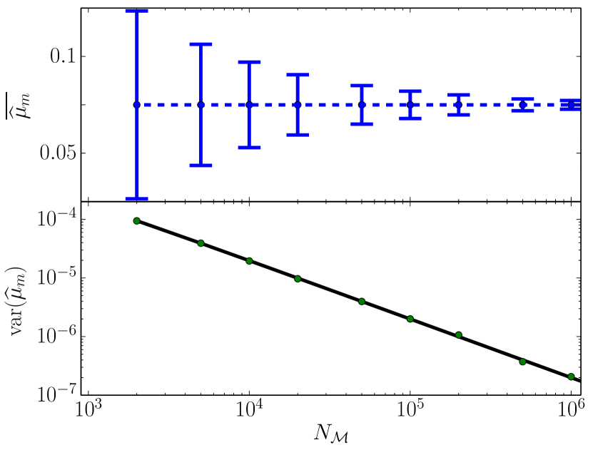
Figure 3: Sample mean (upper panel) and variance (lower panel) of the estimators $\{\widehat{\mu}_{m}\}$ as a function of the partitioned sample size $N_{\mathcal{M}}$, computed from the synthetic time series with $\gamma=0.1$. The dashed line in the upper panel is $\widehat{\mu}$ computed with $N$ data points, the black line in the lower panel is given by Eq. (19).

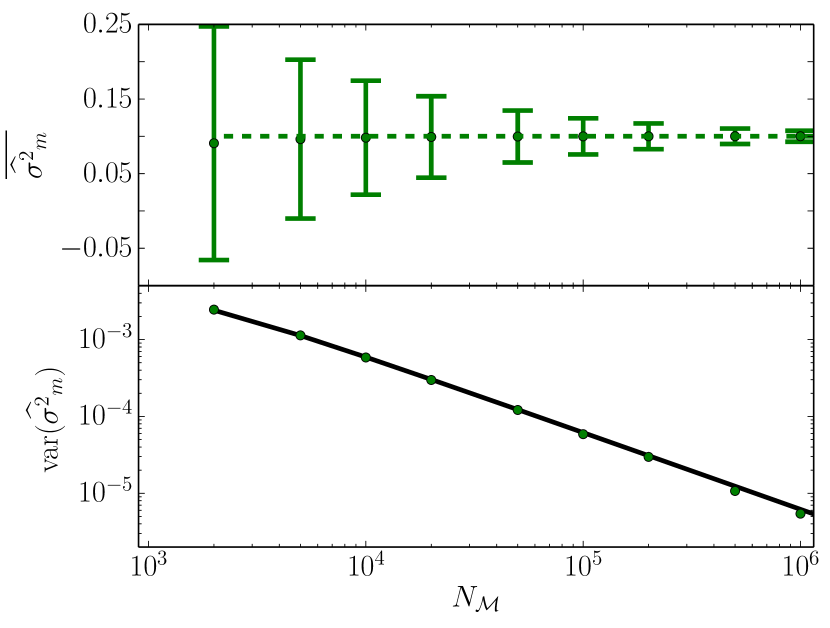
Figure 4: Sample mean (upper panel) and variance (lower panel) of the estimators $\{\widehat{\sigma^{2}}_{m}\}$ computed from the synthetic time series with $\gamma=0.1$. The dashed line in the upper panel is $\widehat{\sigma^{2}}$ computed with $N$ data points, the black line in the lower panel is given by Eq. (23).

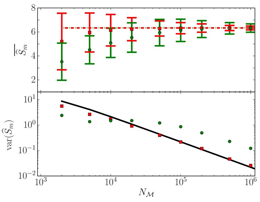
Figure 5: Sample mean (upper panel) and variance (lower panel) of the estimators $\{\widehat{S}_{\Gamma,m}\}$ (red square) and $\{\widehat{S}_{m}\}$ (green circle) computed from the synthetic time series with $\gamma=0.1$. The dashed (dotted) line in the upper panel is $\widehat{S}_{\Gamma}$ ($\widehat{S}$) computed with $N$ data points, the black line in the lower panel is given by Eq. (15).

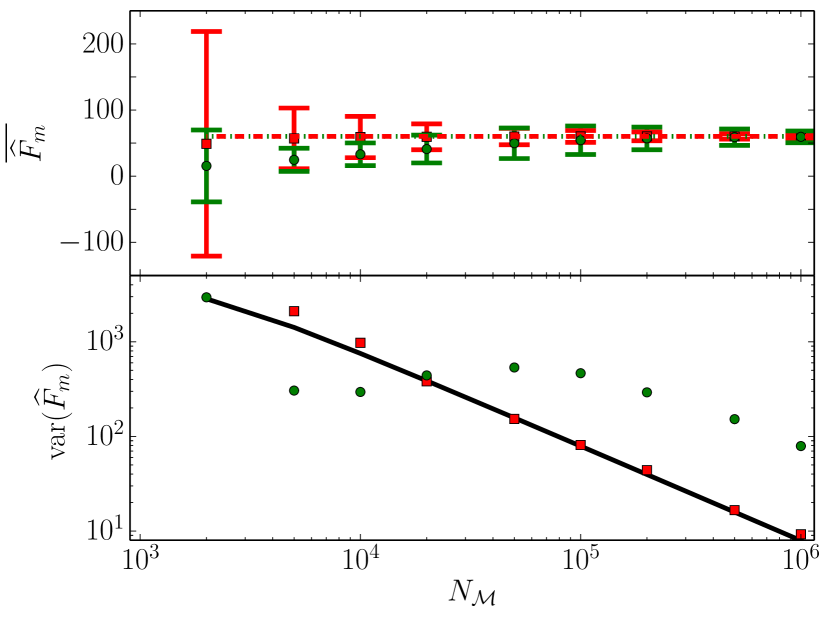
Figure 6: Sample mean (upper panel) and variance (lower panel) of the estimators $\{\widehat{F}_{\Gamma,m}\}$ (red square) and $\{\widehat{F}_{m}\}$ (green circle) computed from the synthetic time series with $\gamma=0.1$. The dashed (dotted) line in the upper panel is $\widehat{F}_{\Gamma}$ ($\widehat{F}$) computed with $N$ data points, the black line in the lower panel is given by Eq. (16).

Figs. 3 - 6 show the results of this comparison for the synthetic time series with $\gamma=0.1$. The upper panel in Fig. 3 shows the sample average of $\{\widehat{\mu}_{m}\}$ with error bars given by the root-mean square of the set for a given sample size $N_{\mathcal{M}}$. Because $\widehat{\mu}$ is linear in all its arguments $x_{i}$ the sample average of $\{\widehat{\mu}_{m}\}$ for any given $N_{\mathcal{M}}$ equals $\widehat{\mu}$ computed for the entire time series. The lower panel compares the sample variance of $\{\widehat{\mu}_{m}\}$ for a given $N_{\mathcal{M}}$ to that given by Eq. (19). For the presented data, the long sample limit applies since $\alpha N_{\mathcal{M}}\geq 20\gg 1$. A least squares fit on $\text{var}(\{\widehat{\mu}_{m}\})$ shows a dependence of $\sim N_{\mathcal{M}}^{-0.90}$ which agrees with the analytical result of $\mathrm{MSE}(\widehat{\mu})\sim N_{\mathcal{M}}^{-1}$, given by Eq. (21).

In Fig. 4 we present the sample average of the estimators $\{\widehat{\sigma^{2}}_{m}\}$ with error bars given by the root-mean square of the set of estimators for a given sample size $N_{\mathcal{M}}$. We find that the sample variance of the estimators compare well with the analytic result given by Eq. (23). A least squares fit reveals that $\text{var}(\{\widehat{\sigma^{2}}_{m}\})\sim N_{\mathcal{M}}^{-0.91}$ while Eq. (23) behaves as $N_{\mathcal{M}}^{-1}$. The sample averages of the skewness estimators $\{\widehat{S}_{\Gamma,m}\}$, Eq. (13), and $\{\widehat{S}_{m}\}$, Eq. (11b), as a function of sample size are shown in the upper panel of Fig. 5. Both estimators yield the same coefficient of skewness when applied to the entire time series and converge to this coefficient with increasing $N_{\mathcal{M}}$. For a small number of samples, $N_{\mathcal{M}}\lesssim 10^{4}$, the estimator based on the method of moments estimates a sample skewness that is on average more than one standard deviation from the true value of skewness. Again, the error bars are given by the root mean square value of the set of estimators for any $N_{\mathcal{M}}$. For larger samples $\text{var}(\{\widehat{S}_{\Gamma,m}\})$ is smaller than $\text{var}(\{\widehat{S}_{m}\})$ by about one order of magnitude and both are inversely proportional to the number of samples. Eq. (15) yields $\mathrm{MSE}(\widehat{S}_{\Gamma})\sim N_{\mathcal{M}}^{-0.99}$ which compares favorably to the dependency of the sample variance of the estimator based on the method of moments on the number of samples, $\text{var}(\{\widehat{S}_{\Gamma,m}\})\sim N_{\mathcal{M}}^{-1.00}$. The discussion of the skewness estimators applies similarly to the kurtosis estimators. Intermittent bursts in the time series with $\gamma=0.1$ cause large deviations from the time series mean which results in a large coefficient of excess kurtosis. Dividing the total time series in sub time series results in large variation of the sample excess kurtosis. For samples with $N_{\mathcal{M}}\lesssim 10^{4}$ the estimator based on the method of moments performs better than the estimator defined in Eq. (13). The opposite is true for samples with $N_{\mathcal{M}}\gtrsim 10^{4}$, where $\widehat{F}_{\Gamma}$ performs significantly better than $\widehat{F}$. In the latter case, $\text{var}(\{\widehat{F}_{\Gamma,m}\})$ is lower than $\text{var}(\{\widehat{F}_{m}\})$ by one order of magnitude. Both estimators, $\widehat{F}$ and $\widehat{F}_{\Gamma}$, converge to their full sample estimate which is identical. A least squares fit reveals that $\text{var}(\{\widehat{F}_{\Gamma,m}\})\sim N_{\mathcal{M}}^{-1.00}$ while a least-squares fit on Eq. (16) finds a dependency of the form $\sim N_{\mathcal{M}}^{-0.97}$.

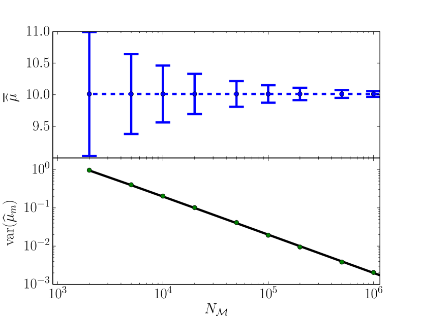
Figure 7: Sample mean (upper panel) and variance (lower panel) of the estimators $\{\widehat{\mu}_{m}\}$ computed from the synthetic time series with $\gamma=10$. The dashed line in the upper panel is $\widehat{\mu}$ computed with $N$ data points, the black line in the lower panel is given by Eq. (19).

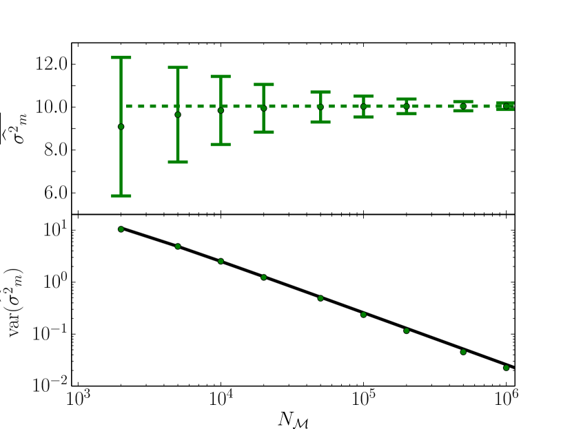
Figure 8: Sample mean (upper panel) and variance (lower panel) of the estimators $\{\widehat{\sigma^{2}}_{m}\}$ computed from the synthetic time series with $\gamma=10$. The dashed line in the upper panel is $\widehat{\sigma^{2}}$ computed with $N$ data points, the black line in the lower panel is given by Eq. (23).

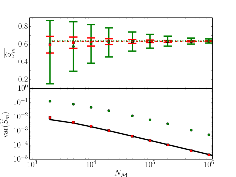
Figure 9: Sample mean (upper panel) and variance (lower panel) of the estimators $\{\widehat{S}_{\Gamma,m}\}$ (red square) and $\{\widehat{S}_{m}\}$ (green circle) computed from the synthetic time series with $\gamma=10$. The dashed (dotted) line in the upper panel is $\widehat{S}_{\Gamma}$ ($\widehat{S}$) computed with $N$ data points, the black line in the lower panel is given by Eq. (15).

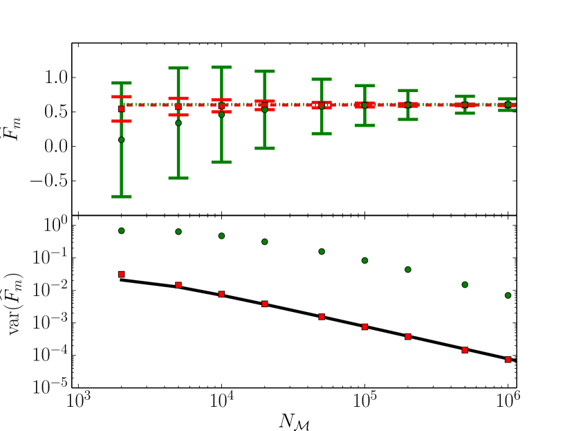
Figure 10: Sample mean (upper panel) and variance (lower panel) of the estimators $\{\widehat{F}_{\Gamma,m}\}$ (red square) and $\{\widehat{F}_{m}\}$ (green circle) computed from the synthetic time series with $\gamma=10$. The dashed (dotted) line in the upper panel is $\widehat{F}_{\Gamma}$ ($\widehat{F}$) computed with $N$ data points, the black line in the lower panel is given by Eq. (16).

In Figs. 7 to 10 we present the same data analysis as in the previous figures, for the time series with a large intermittency parameters, $\gamma=10$. This time series features a large pulse overlap. Again, with $N_{\mathcal{M}}\geq 2\times 10^{3}$, the limit $\alpha N_{\mathcal{M}}\gg 1$ applies. The lower panel in Fig. 7 shows a good agreement between Eq. (23) and the empirical scaling of $\{\widehat{\mu}_{m}\}$ which is found by a least squares fit to be $\text{var}(\{\widehat{\mu}_{m}\})\sim N_{\mathcal{M}}^{-0.98}$, in good agreement with Eq. (21). We further find that $\text{var}(\{\widehat{\sigma^{2}}_{m}\})$ is also inversely proportional to the number of samples, see Fig. 8. For Figs. 9 and 10 we note that the coefficients of skewness and excess kurtosis are one order of magnitude lower for $\gamma=10$ than for $\gamma=0.1$, in accordance with Eq. (6). Due to significant pulse overlap, sample variances of skewness and excess kurtosis show a smaller variance than in the case of $\gamma=0.1$. Again, the magnitude of $\text{var}(\{\widehat{S}_{m}\})$, and $\text{var}(\{\widehat{F}_{m}\})$ is one order of magnitude larger than $\text{var}(\{\widehat{S}_{\Gamma,m}\})$, and $\text{var}(\{\widehat{F}_{\Gamma,m}\})$, respectively, and the variance of all estimators is approximately inversely proportional to $N_{\mathcal{M}}$. For sample sizes up to $N_{\mathcal{M}}\simeq 10^{4}$, $\widehat{F}$ yields negative values for the sample excess kurtosis, while the of excess kurtosis as calculated from the entire sample is positive. This is due to the large sample variance of this estimator and a coefficient of excess kurtosis of the underlying time series.

V Discussions and Conclusion

We have utilized a stochastic model for intermittent particle density fluctuations in scrape-off layer plasmas, given in Ref. LABEL:garcia-2012, to calculate expressions for the mean squared error on estimators of sample mean, variance, coefficients of skewness, and excess kurtosis as a function of sample length, sampling frequency, and parameters of the stochastic process. We find that the mean squared error on the estimator of the sample mean is proportional to the square of the ensemble average of the underlying stochastic process, inversely proportional to the intermittency parameter $\gamma$, and inversely proportional to the number of samples, $N$. In the limit of high sampling frequency and large number of samples, the mean squared error also depends on the ratio of the pulse decay time to sampling frequency, as given by Eq. (21).

The derived expressions for the mean squared error on the estimator for the sample variance and covariance between $\widehat{\mu}$ and $\widehat{\sigma^{2}}$ are polynomials in both $\gamma$ and $N$. These expressions further allow to compute the mean squared error on the sample skewness and excess kurtosis by inserting them into Eqs. (15) and (16). In the limit of high sampling frequency and large number of samples, we find that the expressions for $\mathrm{MSE}(\widehat{\mu})$ and $\mathrm{COV}(\widehat{\mu},\widehat{\sigma^{2}})$ to be inversely proportional to both, $N$, and $\alpha$, and to depend on the intermittency parameter $\gamma$.

We have generated synthetic time series to compare the sample variance of the estimators for sample mean, variance, skewness and excess kurtosis to the expressions for their mean squared error. For a large enough number samples, $\alpha N\gg 1$, all estimators are inversely proportional to $N$. We further find that estimators for skewness and excess kurtosis, as defined by Eq. (13), allow a more precise and a more accurate estimation of the sample skewness and kurtosis than estimators based on the method of moments given by Eq. (11b).

The expressions given by Eqs. (19), (23), (15), and (16) may be directly applied to assess the relative error on sample coefficients of mean, variance, skewness, and kurtosis for time series of particle density fluctuations in tokamak scrape-off layer plasmas. We exemplify their usage for a particle density time series that is sampled with $1/\triangle_{t}=5\,\mathrm{MHz}$ for $T=2.5\,\mathrm{ms}$ as to obtain $N=12500$ samples. Common fluctuation levels in the scrape-off layer are given by $\Phi_{\mathrm{rms}}/\langle\Phi\rangle\approx 0.5$. Using Eq. (6a) and $\gamma=\tau_{\mathrm{d}}/\tau_{\mathrm{w}}$, this gives $\gamma\approx 4$. Conditional averaging of the the bursts occurring in particle density time series reveals an exponentially decaying burst shape with a typical e-folding time of approximately $20\,\mu\mathrm{s}$, so that $\alpha\approx 0.01$. Thus, the individual bursts are well resolved on the time scale on which the particle density is sampled and the assumption $\alpha N\gg 1$ is justified. From Eq. (21), we then compute the relative mean squared error on the sample average to be $\mathrm{MSE}(\widehat{\mu})/\langle\Phi\rangle^{2}\simeq 3.2\times 10^{-3}$ and likewise the relative mean squared error on the sample variance from Eq. (26) to be $\mathrm{MSE}(\widehat{\sigma^{2}})/\text{var}\left(\Phi\right)^{2}\simeq 2.6\times 10^{-2}$. This translates into relative errors of approximately $6\%$ on the sample mean and approximately $16\%$ on the sample variance. The relative mean squared error on skewness and excess kurtosis evaluates to $\mathrm{MSE}(\widehat{S}_{\Gamma})/\widehat{S}_{\Gamma}^{2}\simeq 8.6\times 10^{-3}$ and $\mathrm{MSE}(\widehat{F}_{\Gamma})/\widehat{F}_{\Gamma}^{2}\simeq 3.8\times 10^{-2}$, which translates into an relative error of approximately $9\%$ on the sample skewness and approximately $19\%$ on the sample excess kurtosis. The magnitude of these values is consistent with reported radial profiles os sample skewness and kurtosis, where the kurtosis profiles show significantly larger variance than the skewness profiles LABEL:garcia-2007-tcv,_graves-2005,_horacek-2005,_garcia-2006-tcv,_garcia-2007-coll.

The expressions for the mean squared error on sample mean, variance, skewness and kurtosis presented here may be appropriate for errorbars on experimental measurements of particle density fluctuations, as well as for turbulence simulations of the boundary region of magnetically confined plasmas.

Appendix A Derivation of $\mathrm{MSE}(\widehat{\sigma^{2}})$ and $\mathrm{COV}(\widehat{\mu},\widehat{\sigma^{2}})$

We start by reminding of the definitions $\mathrm{COV}(\widehat{A},\widehat{B})=\langle(\widehat{A}-\langle A\rangle)(\widehat{B}-\langle B\rangle)\rangle$ and $\mathrm{var}(\widehat{B})=\langle(\widehat{B}-\langle B\rangle)^{2}\rangle$. For $\widehat{A}=\widehat{\mu}$ and $\widehat{B}=\widehat{\sigma^{2}}$, we evaluate these expressions to be

$$\mathrm{COV}(\widehat{\mu},\widehat{\sigma^{2}}) =\frac{1}{N-1}\left(\sum\limits_{i,j=1}^{N}\langle\Phi(t_{i})^{2}\Phi(t_{j})\rangle-\frac{1}{N^{2}}\sum\limits_{i,j,k=1}^{N}\langle\Phi(t_{i})\Phi(t_{j})\Phi(t_{k})\rangle\right)$$

$$\quad-\langle A\rangle\frac{\tau_{\mathrm{d}}}{\tau_{\mathrm{w}}}\frac{1}{N-1}\left(\sum\limits_{i=1}^{N}\langle\Phi(t_{i})\rangle-\frac{1}{N}\sum\limits_{i,j=1}^{N}\langle\Phi(t_{i})\Phi(t_{j})\rangle\right),$$ (27)

and

$$\mathrm{var}(\widehat{\sigma^{2}}) =-\langle A\rangle^{4}\left(\frac{\tau_{\mathrm{d}}}{\tau_{\mathrm{w}}}\right)^{2}+4\langle A\rangle^{4}\left(\frac{\tau_{\mathrm{d}}}{\tau_{\mathrm{w}}}\right)^{2}\left(\frac{1}{N^{2}}\frac{e^{-\alpha N}-(1-\alpha N)}{\alpha^{2}}\right)$$

$$+\frac{1}{N^{2}}\left(\sum\limits_{i,j=1}^{N}\langle\Phi(t_{i})^{2}\Phi(t_{j})^{2}\rangle\right.\left.-\frac{2}{N}\sum\limits_{i,j,k=1}^{N}\langle\Phi(t_{i})^{2}\Phi(t_{j})\Phi(t_{k})\rangle\right.$$

$$\left.\hskip 43.05542pt+\frac{1}{N^{2}}\sum\limits_{i,j,k,l=1}^{N}\langle\Phi(t_{i})\Phi(t_{j})\Phi(t_{k})\Phi(t_{l})\rangle\right)$$ (28)

We made use of Eq. (22) in deriving the last expression. Therefore it is only valid in the limit $\alpha\ll 1$. To derive closed expressions for Eqs. (15) and (16) we proceed by deriving expressions for the third- and fourth-order correlation functions of the shot noise process Eq. (1).

We start by inserting Eq. (1) into the definition of a three-point correlation function

$$\langle\Phi_{K}(t)\Phi_{K}(t+\tau)\Phi_{K}(t+\tau^{\prime})\rangle$$

$$=\int\limits_{0}^{T}\mathrm{d}t_{1}P_{t}(t_{1})\int\limits_{0}^{\infty}\mathrm{d}A_{1}P_{A}(A_{1})\cdots\int\limits_{0}^{T}\mathrm{d}t_{1}PKt(t_{K})\int\limits_{0}^{\infty}\mathrm{d}A_{K}P_{A}(A_{K})\times$$

$$\qquad\sum\limits_{p=1}^{K}\sum\limits_{q=1}^{K}\sum\limits_{r=1}^{K}A_{p}\psi(t-t_{p})A_{q}\psi(t+\tau-t_{q})A_{r}\psi(t+\tau^{\prime}-t_{r})$$

$$=\langle A^{3}\rangle\sum\limits_{p=q=r=1}^{K}\int\limits_{0}^{T}\frac{\mathrm{d}t_{p}}{T}\psi(t-t_{p})\psi(t+\tau-t_{p})\psi(t+\tau^{\prime}-t_{p})$$

$$\qquad+\langle A^{2}\rangle\langle A\rangle\sum\limits_{p=q=1}^{K}\sum\limits_{\begin{subarray}{c}r=1\\ r\neq p\end{subarray}}^{K}\int\limits_{0}^{T}\frac{\mathrm{d}t_{p}}{T}\int\limits_{0}^{T}\frac{\mathrm{d}t_{r}}{T}\psi(t-t_{p})\psi(t+\tau-t_{p})\psi(t+\tau^{\prime}-t_{r})$$

$$\qquad+\langle A^{2}\rangle\langle A\rangle\sum\limits_{p=r=1}^{K}\sum\limits_{\begin{subarray}{c}q=1\\ q\neq p\end{subarray}}^{K}\int\limits_{0}^{T}\frac{\mathrm{d}t_{p}}{T}\int\limits_{0}^{T}\frac{\mathrm{d}t_{q}}{T}\psi(t-t_{p})\psi(t+\tau-t_{q})\psi(t+\tau^{\prime}-t_{p})$$

$$\qquad+\langle A^{2}\rangle\langle A\rangle\sum\limits_{q=r=1}^{K}\sum\limits_{\begin{subarray}{c}p=1\\ p\neq r\end{subarray}}^{K}\int\limits_{0}^{T}\frac{\mathrm{d}t_{q}}{T}\int\limits_{0}^{T}\frac{\mathrm{d}t_{p}}{T}\psi(t-t_{p})\psi(t+\tau-t_{q})\psi(t+\tau^{\prime}-t_{q})$$

$$\qquad+\langle A\rangle^{3}\sum\limits_{p=1}^{K}\sum\limits_{q=1}^{K}\sum\limits_{r=1}^{K}\int\limits_{0}^{T}\frac{\mathrm{d}t_{p}}{T}\int\limits_{0}^{T}\frac{\mathrm{d}t_{q}}{T}\int\limits_{0}^{T}\frac{\mathrm{d}t_{r}}{T}\psi(t-t_{p})\psi(t+\tau-t_{q})\psi(t+\tau^{\prime}-t_{r}).$$ (29)

The sum over the product of the individual pulses is grouped into six sums. The first sum contains factors with equal pulse arrival times and consists of $K$ terms. The next three groups contain terms where two pulses occur at the same arrival time, each group counting $K(K-1)$ terms. The last sum contains the remaining $K(K-1)(K-2)$ terms of the terms where all three pulses occur at different pulse arrival times.

The sum occurring in the four point correlation function may be grouped by equal pulse arrival time as well. In the latter case, the sum may be split up into group of terms where four, three and two pulse arrival times are equal, and in a sum over the remaining terms. The sums in each group have $K$, $K(K-1)$, $K(K-1)(K-2)$, and $K(K-1)(K-2)(K-3)$ terms respectively.

Similar to Eq. (8), we evaluate the integral of the product of three pulse shapes while neglecting boundary terms to be

$$\int\limits_{0}^{T}\mathrm{d}t_{p}P_{t}(t_{p}) \psi(t-t_{p})\psi(t+\tau-t_{p})\psi(t+\tau^{\prime}-t_{p})$$

$$\simeq\frac{\tau_{\mathrm{d}}}{3}\exp\left(\frac{\tau+\tau^{\prime}}{\tau_{\mathrm{d}}}\right)\exp\left(-3\frac{\max\left(0,\tau,\tau^{\prime}\right)}{\tau_{\mathrm{d}}}\right)$$ (30)

while the integral of the product of four pulse shapes is given by

$$\int\limits_{0}^{T}\mathrm{d}t_{p}P_{t}(t_{p}) \psi(t-t_{p})\psi(t+\tau-t_{p})\psi(t+\tau^{\prime}-t_{p})\psi(t+\tau^{\prime\prime}-t_{p})$$

$$\simeq\frac{\tau_{\mathrm{d}}}{4}\exp\left(\frac{\tau+\tau^{\prime}+\tau^{\prime\prime}}{\tau_{\mathrm{d}}}\right)\exp\left(-4\frac{\max\left(0,\tau,\tau^{\prime},\tau^{\prime\prime}\right)}{\tau_{\mathrm{d}}}\right).$$ (31)

To obtain an expression for the third- and fourth-order correlation functions, these integrals are inserted into the correlation function and the resulting expression is averaged over the total number of pulses. We point out that the $K$ pulses occurring in the time interval $[0:T]$ is Poisson distributed and that for a Poisson distributed random variable $K$,

$$\left\langle\prod\limits_{n=0}^{z}K-n\right\rangle=K^{z}$$

holds. Using this with $Z=2$, the three-point correlation function evaluates to

$$\langle\Phi(t)\Phi(t+\tau)\Phi(t+\tau^{\prime})\rangle =\langle A\rangle^{2}\left[2\frac{\tau_{\mathrm{d}}}{\tau_{\mathrm{w}}}\exp\left(\frac{\tau+\tau^{\prime}}{\tau_{\mathrm{d}}}-3\frac{\max(0,\tau,\tau^{\prime})}{\tau_{\mathrm{d}}}\right)\right.$$

$$\left.+\left(\left(\frac{\tau_{\mathrm{d}}}{\tau_{\mathrm{w}}}\right)^{2}+1\right)\exp\left(\frac{\tau}{\tau_{\mathrm{d}}}-2\frac{\max(0,\tau)}{\tau_{\mathrm{d}}}\right)+\left(\frac{\tau_{\mathrm{d}}}{\tau_{\mathrm{w}}}\right)^{3}\right].$$ (32)

The four-point correlation function is evaluated the same way.

To evaluate summations over higher-order correlation function, we note that Eq. (32) evaluated at discrete times can be written as

$$\langle\Phi(t_{i})\Phi(t_{j})\Phi(t_{k})\rangle =\langle A\rangle^{2}\left[2\left(\frac{\tau_{\mathrm{d}}}{\tau_{\mathrm{w}}}\right)\exp\Bigl{(}\alpha(2i-j-k)-3\alpha\max(0,i-j,j-k)\Bigr{)}\right.$$

$$\left.+\left(\left(\frac{\tau_{\mathrm{d}}}{\tau_{\mathrm{w}}}\right)^{2}+1\right)\exp\Bigl{(}\alpha(i-j)-\max(0,i-j)\Bigr{)}+\left(\frac{\tau_{\mathrm{d}}}{\tau_{\mathrm{w}}}\right)^{3}\right],$$ (33)

where $\tau=\tau_{ij}=\triangle_{t}\left(i-j\right)$ and $\tau^{\prime}=\tau_{jk}=\triangle_{t}\left(j-k\right)$. The summations over higher-order correlation functions in Eq. (27) and Eq. (28) may then be evaluated by approximating the sums by an integral, assuming $N\gg 1$, and dividing the integration domain into sectors where $i<j<k$, $i<k<j$, $\ldots$. In each of these sectors, the $\max$-functions in Eq. (33) are secular valued so that the integral is well defined. Denoting all permutations of the tuple $(i,j,k)$ as $\mathcal{P}_{3}$, and the respective elements of a permutated tuple as $\pi_{1}$, $\pi_{2}$, $\pi_{3}$, we thus have

$$\sum\limits_{i,j,k=1}^{N}\langle\Phi(t_{i})\Phi(t_{j})\Phi(t_{k})\rangle \simeq\int\limits_{0}^{N}\mathrm{d}i\,\mathrm{d}j\,\mathrm{d}k\,\langle\Phi(t_{i})\Phi(t_{j})\Phi(t_{k})\rangle\times\left(\sum\limits_{\pi\in\mathcal{P}_{3}}\Theta(\pi_{1}-\pi_{2})\Theta(\pi_{2}-\pi_{3})\right)$$

$$\sum\limits_{i,j,k,l=1}^{N}\langle\Phi(t_{i})\Phi(t_{j})\Phi(t_{k})\Phi(t_{l})\rangle \simeq\int\limits_{0}^{N}\mathrm{d}i\,\mathrm{d}j\,\mathrm{d}k\,\mathrm{d}l\,\langle\Phi(t_{i})\Phi(t_{j})\Phi(t_{k})\Phi(t_{l})\rangle\times$$

$$\left(\sum\limits_{\pi\in\mathcal{P}_{4}}\Theta(\pi_{1}-\pi_{2})\Theta(\pi_{2}-\pi_{3})\Theta(\pi_{3}-\pi_{4})\right).$$

These integral are readily evaluated. Inserting them into Eq. (27), and Eq. (28), yields the expression Eq. (24) and Eq. (23).

References

• (1) The expected value of the sample coefficient of kurtosis for a sample drawn from a normal distribution is three. The sample coefficient of excess kurtosis is found by subtracting 3 from the sample coefficient of kurtosis, see Eq. (11b)
• (2) G.Y. Antar, P. Devynck, X. Garbet, and S.C. Luckhardt, Phys. Plasmas 8, 1612 (2001).
• (3) G.Y. Antar, G. Counsell, Y. Yu, B. LaBombard, and P. Devynck, Phys. Plasmas 10, 419 (2003).
• (4) J.M. Dewhurst, B. Hnat, N. Ohno, R.O. Dendy, S. Masuzaki, T. Morisaki, and A. Komori, Plasma Phys. Controlled Fusion 50, 095013 (2008).
• (5) Y.H. Xu, S. Jachmich, R.R. Weynants, and the TEXTOR team, Plasma Phys. Controlled Fusion 47, 1841 (2005).
• (6) M. Agostini, S.J. Zweben, R. Cavazzana, P. Scarin, G. Serianni, R.J. Maqueda, and D.P. Stotler, Phys. Plasmas 14 102305 (2007).
• (7) J.A. Boedo, D.L. Rudakov, R.A. Moyer, G.R. McKee, R.J. Colchin, M.J. Schaffer, P.G. Stangeby, W.P. West, S.L. Allen, T.E. Evans, R.J. Fonck, E.M. Hollmann, S. Krasheninnikov, A.W. Leonard, W. Nevins, M.A. Mahdavi, G.D. Porter, G.R. Tynan, D.G. Whyte, and X. Xu, Phys. Plasmas 10, 1670 (2003).
• (8) J. Cheng, L.W. Yan, W.Y. Hong, K.J. Zhao, T. Lan, J. Qian, A.D. Liu, H.L. Zhao, Y. Liu, Q.W. Yang, J.Q. Dong, X.R. Duan, and Y. Liu, Plasma Phys. Controlled Fusion 52, 055033 (2010).
• (9) B. Nold, G.D. Conway, T. Happel, H.W. Müller, M. Ramisch, V. Rohde, U. Stroth, and the ASDEX Upgrade Team, Plasma Phys. Controlled Fusion 52, 065005 (2010).
• (10) H. Tanaka, N. Ohno, N. Asakura, Y. Tsuji, H. Kawashima, S. Takamura, Y. Uesugi, and the JT-60U Team, Nucl. Fusion 49, 065017 (2009).
• (11) G.S. Xu, V. Naulin, W. Fundamenski, C. Hidalgo, J.A. Alonso, C. Silva, B. Gonçalves, A.H. Nielsen, J. Juul Rasmussen, S.I. Krasheninnikov, B.N. Wan, M. Stamp, and JET EFDA Contributors, Nucl. Fusion 49, 092002 (2009).
• (12) O.E. Garcia, J.Horacek, R.A. Pitts, A.H. Nielsen, W. Fundamenski, V. Naulin, and J. Juul Rasmussen, Nucl. Fusion 47, 667 (2007);
O.E. Garcia, R. A. Pitts, J. Horacek, A.H. Nielsen, W. Fundamenski, J.P. Graves, V. Naulin and J. Juul Rasmussen, Journ. Nucl. Mat. 363-365, 575 (2007).
• (13) D.A. Russell, J.R.Myra, and D.A. D’Ippolito, Phys. Plasmas 14, 102307 (2007).
• (14) J.R. Myra, D.A. Russell, and D.A. D’Ippolito, Phys. Plasmas 15, 032304 (2008).
• (15) F. Militello, W. Fundamenski, V. Naulin, and A.H. Nielsen, Plasma Phys. Controlled Fusion 54 095011 (2012).
• (16) K.P. Balanda, and H.L. MacGillivray, The Amer. Statistician 42, 111 (1988).
• (17) O.E. Garcia, S.M. Fritzner, R. Kube, I. Cziegler, B. LaBombard, and J.L. Terry, Phys. Plasmas 20, 055901 (2013); O.E. Garcia, I. Cziegler, R. Kube, B. LaBombard, and J.L. Terry, Journ. Nucl. Mat. 438, S180 (2013).
• (18) J.P.Graves, J.Horacek, R.A.Pitts, and K.I. Hopcraft, Plasma Phys. Controlled Fusion 47, L1 (2005).
• (19) B. Labit, I. Furno, A. Fasoli, A. Diallo, S.H. Müller, G. Plyushchev, M. Podestà, and F.M. Poli, Phys. Rev. Lett. 98, 255002 (2007).
• (20) F. Sattin, P. Scarin, M. Agostini, R. Cavazzana, G. Serianni, M. Spolaore, and N. Vianello, Plasma Phys. and Controlled Fusion 48, 1033 (2006).
• (21) J. Rice, Adv. Appl. Prob. 9, 553-565 (1977).
• (22) O.E.Garcia, Phys. Rev. Lett. 108, 265001 (2012).
• (23) O.E.Garcia, J.Horacek, R.A. Pitts, A.H. Nielsen, W. Fundamenski, J. P. Graves, V. Naulin, and J. Juul Rasmussen, Plasma Phys. Controlled Fusion 48, L1 (2006).
• (24) S. J. Zweben, D. P. Stotler, J. L. Terry, B. LaBombard, M. Greenwald, M. Muterspaugh, C. S. Pitcher, the Alcator C-Mod Group, K. Hallatschek, R. J. Maqueda, B. Rogers, J. L. Lowrance, V. J. Mastrocola, and G. F. Renda, Phys. Plasmas 9, 1981 (2002).
• (25) D.P. Stotler, B. LaBombard, J.L. Terry, and S.J. Zweben, Journ. Nucl. Mat. 313-316, 1066 (2003).
• (26) I. Cziegler Turbulence and Transport Phenomena in Edge and Scrape-Off-Layer Plasmas, Ph.D. thesis, Massachusetts Institute of Technology (2011).
• (27) H.L. Pecseli, Fluctuations in Physical systems Cambridge University Press (2000).
• (28) O.E. Garcia, Plasma Fusion Research 4, 019 (2009).
• (29) G. Furchert, G. Birkenmeier, B. Nold, M. Ramisch, and U. Stroth, Plasma Phys. Controlled Fusion 55, 125002 (2013).
• (30) J. Horacek, R.A. Pitts, and J.P. Graves, Czech. Journ. Phys. 55, 271 (2005)
• (31) O.E. Garcia, R.A. Pitts, J. Horacek, J. Madsen, V. Naulin, A.H. Nielsen, and J. Juul Rasmussen, Plasma Phys. and Controlled Fusion 49, B47 (2007)
• (32) N. Bian, S. Benkadda, J.V. Paulsen, and O.E. Garcia, Phys. Plasmas 10, 671 (2003)
• (33) O.E. Garcia, N. Bian and W. Fundamenski, Phys. Plasmas 13 082309 (2006)
• (34) R. Kube and O.E. Garcia, Phys. Plasmas 18 102314 (2011); Phys. Plasmas 19 042305 (2012).
Refer to caption