Parameter switching in a generalized Duffing system: Finding the stable attractors

Abstract

This paper presents a simple periodic parameter-switching method which can find any stable limit cycle that can be numerically approximated in a generalized Duffing system. In this method, the initial value problem of the system is numerically integrated and the control parameter is switched periodically within a chosen set of parameter values. The resulted attractor matches with the attractor obtained by using the average of the switched values. The accurate match is verified by phase plots and Hausdorff distance measure in extensive simulations.

Keyword Parameter switching; Duffing system; Hausdorff distance;

Mathematics Subject Classification: 34D45, 37C60, 70K05

1 Introduction

The well-known Duffing system was coined in 1918, which is one of the mostly studied nonlinear dynamical systems describing mechanical structures, and electric circuits and even biological re systems. This paper considers a generalized Duffing system of the form

$$\overset{..}{x}+a\overset{.}{x}+px+bx^{3}+c~{}sign(x)+d~{}sign(\overset{.}{x})=e~{}\cos\left(\omega t\right),$$ (1)

where $a,b,c,d,e,\omega$ and $p$ (considered as the control parameter) are real parameters. As for almost all practical examples, at least one of the parameters, $c$ and $d$, will be zero. Thus, according to different functions of $c$ and $d$, one could have the classical form of excited Duffing oscillator ($c=d=0$), dry friction models ($c=0,d=1$), or other phenomena such as clearance, vibro-impacts, and preloaded compliance ($c=1,d=0$). The external force is typically considered to be periodic, since the study of the long-term behavior of an oscillator is relevant only in this setting.

Duffing’s smooth and discontinuous dynamics are a very good examples for demonstrating how deterministic chaos appears in mechanical systems that may be described as oscillators derived from a nonlinear potential. For illustration, routes to chaos through bifurcations are shown in Fig.1. There exists a large volume of bibliography on the rich dynamics of the Duffing oscillator, some of the first titles being [13, 28] and [20], while experimental implementations of the Duffing system can be found in many references, e.g. [19].

Many non-smooth systems appear naturally in practical systems because such physical phenomena present discontinuities, for instance the discontinuous dependence of friction force on the velocity, mechanical structures under impacts and dry friction, brake processes with phase lock, oscillating systems with combined dry and viscous damping, elasto-plasticity and forced vibrations. Also they appear in power electrical circuits, convex optimization, control synthesis of uncertain systems, walking and hopping robots, and even gene regulatory networks and neuronal networks, etc. [2, 3, 9, 21, 22, 23, 24, 26, 29]. Noticeably, a large number of papers are devoted to studying the fundamentals of discontinuous equations (such as (1)) or to the afferent differential inclusions which help tackle various difficult discontinuous problems [1, 11, 15, 16]. These studies clearly indicate that dry friction and its underlying discontinuity present an important topic in both mathematical and engineering research.

Motivated by the above observations, considering the system (1) with discontinuity appears to be a natural approach to more realistic engineering systems design and analysis. The present paper therefore investigates an important and yet challenging problem in this system, more precisely a problem of approximating (synthesizing) any stable attractor in system (1) by alternating parameter $p$ within a set of chosen values while the system is numerically integrated.

For this purpose, we will use the Parameter Switching (PS) algorithm. This algorithm is very effective in approximating various complex dynamical behaviors corresponding to the switched parameter, such as multiple attractors. It has been analytically proved [17, 18] that for a large class of continuous systems, any synthesized attractor obtained by using this algorithm can well match with the attractor obtained by replacing $p$ with the average of the alternated $p$ values. This has also been verified numerically applicable to more general classes of dynamical systems. Moreover, the effectiveness of the PS algorithm has been tested on several systems, including continuous, discontinuous, and fractional or integer order systems [5, 7]), such as Lorenz, Rössler, Chen, Chua, Lü, Lotka Volterra, and Hindmarsh-Rose neuronal systems, among others.

System (1) is solved mathematically by the following general Initial Value Problem (IVP):

$$\overset{.}{x}=f(x)+pAx+Bs(x),~{}x(0)=x_{0},~{}t\in I=[0,\infty).$$ (2)

This shows that the system depends linearly on $p$, same as for the general class of many known systems like the Lorenz, Chen, Rössler, Chua, Hindmarsh-Rose, Lotka Volterra systems. In (2, $p\in\mathbb{R}$, $x\in\mathbb{R}^{n}$, $A,B\in\Re^{n\times n}$ are constant matrices, $~{}f:\mathbb{R}^{n}\rightarrow\mathbb{R}^{n}$ is a nonlinear at least continuous vector function, and $s:\mathbb{R}^{n}\rightarrow\mathbb{R}^{n}$ is a vector piecewise linear vector function being composed of scalar signum functions, namely

$$s(x)=\left(\begin{array}[]{c}sgn(x_{1})\\ \vdots\\ sgn(x_{n})\end{array}\right).$$

Function of the entries of the matrix $B$, the IVP (2) can model continuous systems (when $B=O_{n\times n}$) or discontinuous with respect to the state variable (Filippov like systems [11], when $B\neq O_{n\times n}$).

Now, consider the Duffing oscillator (1) in the phase space $\mathbb{R}^{3}$ having the following three autonomous equations:

$$\begin{array}[]{l}\overset{.}{x}_{1}=x_{2},\\ \overset{.}{x}_{2}=-ax_{2}-px_{1}-bx_{1}^{3}-c~{}sign(x_{1})-d~{}sign(x_{2})+e\cos\left(x_{3}\right),\\ \overset{.}{x}_{3}=\omega.\end{array}$$ (3)

It can be easily seen that this belongs to the class of systems described by the IVP (2) with

$$\begin{array}[]{c}f(x)=\left(\begin{array}[]{c}x_{2}\\ -ax_{2}-bx_{1}^{3}+e\cos\left(x_{3}\right)\\ \omega\end{array}\right),~{}A=\left(\begin{array}[]{ccc}0&0&0\\ -1&0&0\\ 0&0&0\end{array}\right),~{}~{}B=\left(\begin{array}[]{ccc}0&0&0\\ -c&-d&0\\ 0&0&0\end{array}\right).\end{array}$$

Even the system (3) is three-dimensional, so our interest here is focused, on the phase plane $\left(x_{1},x_{2}\right)$, as usually for planar systems.

We will investigate the effect of the positive parameter $p$. For the others parameters, we chose:

$a=1$ i.e. the case of a strong dissipation (damped oscillations), in order to avoid long chaotic transients, typical for weak dissipation (as known, chaotic behaviors could persist for some transient time before the trajectory approach near the attractor [14]);

$b=1$;

$c$ and $d$ are chosen $0$ or $1$ corresponding to the continuous or discontinuous case.

$e=37$ (the amplitude of the driving forces on oscillations $x$);

$\omega=0.88$.

2 Attractors synthesis

2.1 Preliminary results and notions

Notation 1. Let $P_{N}=\{p_{1},p_{2},...,p_{N}\}$ a set of $N>0$ values of $p$. The average value, denoted by $p^{*}$ is given by

$$p^{\ast}=\frac{\sum\limits_{k=1}^{N}p_{k}m_{k}}{\sum\limits_{k=1}^{N}m_{k}},$$ (4)

where $m_{i}$ are some positive integers, which will be precisely defined later.

2. We denote the attractors obtained through alternating $p$ with the PS algorithm, the synthesized attractor, by $A^{*}$ and the average attractor by $A_{p^{*}}$, corresponding to $p=p^{*}$.

Remark 1.

In different functions on $m_{k}$ values in (4), $p^{*}$ could be an element of $\mathcal{P}_{N}$. However, in this paper we consider that $p^{*}\notin\mathcal{P}_{N}$, since in practical examples it is more realistic to approximate an attractor $A_{p^{*}}$ starting from a set $P_{N}$ which does not contain $p^{*}$.

To understand how the PS algorithm works, we further consider the general problem (2) for the continuous case ($B=0_{n\times n}$), with a time-dependent $p$, as follows:

$$\dot{x}(t)=f(x(t))+p\left(t\right)Ax(t),~{}~{}x(t_{0})=x_{0},~{}~{}t\in I,$$ (5)

where $p:I\rightarrow P_{N}$ is considered a piecewise constant periodic function with the period $T_{0}$, and the the mean value $p^{*}$, namely,

$$\frac{1}{T_{0}}\int_{t}^{t+T_{0}}p(u)du=p^{*},\qquad t\in I.$$

also, the average model of (5), is expressed as follows;

$$\dot{y}=f(y)+p^{*}Ay,~{}~{}y(0)=y_{0}.$$ (6)

Equation (5) represents the mathematical model of the PS algorithm.

In additiona, we need the following assumptions.

(H1) The IVP admits unique solutions (e.g., when $f$ is Lipschitz continuous).

(H2) To each $p$ value, there corresponds a single attractor which will be numerically approximated by its $\omega$-limit set [12], after neglecting a sufficiently long period of transients.

(H3) The initial conditions $x_{0}$ and $y_{0}$ in (5) and (6), respectively, are chosen close enough to each other (in the same basin of attraction).

Now, we can introduce the following theorem (proved in $\mathbb{R}^{n}$ [17, 18]).

Theorem 1.

The solution of Equation (5) approaches the solution of Equation (6).

The proof presented in [17] is based on the averaging theory [25], and is done via generalized Péano-Baker series, while the proof presented in [18] uses the convergence of known numerical methods for ODEs.

Thus, it is proved that the distance between the solutions of linearized Equation (5) and of Equation (6), starting from the same basin of attraction, is negligible. Therefore, we have revealed (see also [27], Chapter 6) that the invariant sets of system (5), determined numerically, converge to the invariant sets of system (6). This means that the PS algorithm, modeled by (5), is approximated by periodical parameter switching and that the attractor corresponding to $p^{*}$ is generated by (6).

To Summarize, by switching $p$ periodically while the IVP is numerically integrated, one obtains a synthesized attractor, $A^{*}$, which matches with the attractor $A_{p^{*}}$ obtained when $p$ is replaced by $p^{*}$.

The PS algorithm is useful in practical examples when one intends to obtain some attractor $A^{*}$, but its underlying parameter $p^{*}$ cannot be set. Thus, $p^{*}$ and the corresponding attractor $A_{p^{*}}$ will be obtained by switching $p$ within some accessible set of values $\mathcal{P}_{N}$.

2.2 Numerical implementation

Theorem 1 only proves that the PS algorithm convergences to some attractor $A^{*}$, which approximates the attractor $A_{p^{*}}$, but it does not indicate any way to implement it in concrete examples. Therefore, a numerical modality to implement this result is necessary. For this purpose, two steps are formulated:

I) run the PS algorithm, which generates a synthesized attractor $A^{*}$ via parameter switching;

II) show numerically (aided by characteristic tools for dynamical systems) that $A^{*}$ matches with the average attractor $A_{p^{*}}$ obtained when $p$ is replaced by the average value $p^{*}$.

Remark 2.

(i) Step II is necessary in order to prove that $A^{*}$ is not just an attractor, but it belongs to the set of attractors of the underlying system.

(ii) Due to the predominant numerical characteristics of the present work, the time interval $I$ is considered hereafter finite: $I=[0,T]$, with $T>0$.

(iii) Regarding the approach to the discontinuous case, it is noted that the underlying IVP can be continuously approximated in some neighborhood of the discontinuity point (here, $x_{1}=0$ and $x_{2}=0$), using e.g. the Filippov regularization [11]. After this, the PS algorithm is applied, as described for the continuous case (see [8]). Thus, the problem is transformed to a continuous one, where the PS algorithm is applicable.

In order to reduce the number of transient steps and to avoid possible complication when, for a given $p$ value, there are several (coexisting) attractors, the initial conditions will be taken without loss of generality to be $x_{0}=y_{0}$.

Let us again consider the simpler case of continuous Duffing system ($B=0_{n\times n}$, i.e. $c=d=0$).

I) To implement the PS algorithm, a numerical method for ODEs such as the standard Runge-Kutta method with a fixed step seize $h$, will be used. Suppose we chose $P_{N}$, and $p$ is switched indefinitely within $P_{N}$ for $t<T$, in the following manner

$$p(t)=p_{i}~{}~{}if~{}~{}t\in I_{i},~{}p_{i}\in P_{N},~{}i=1,2,...,N,\\$$

where the time subintervals $I_{i}$, $i=1,2,...,N$, obtained by partition of $I$, satisfy $I=\bigcup\left(\bigcup_{k=1}^{N}I_{k}\right)$.

The simplest way to realize that, numerically, is to choose the length of $I_{i}$ as a multiple of $h$: $I_{i}=m_{i}h$, where $m_{i},~{}i=1,2,...,N$, are some positive integers (”weights”).

Denote the PS algorithm, for a step size $h$, as follows

$$[m_{1}p_{1},m_{2}p_{2},...,m_{N}p_{N}].$$ (7)

The pseudocode for PS algorithm is presented in Table 1.

For example, by $[1p_{1},2p_{2}]$, we understand that PS, with $N=2$, $P_{2}=\{p_{1},p_{2}\}$, $m_{1}=1$ and $m_{2}=2$, integrates the IVP for one step of size $h$ with $p=p_{1}$. Then, perform the next two steps with $p=p_{2}$ and again one step with $p=p_{1}$; after that, perform two steps $p=p_{2}$ and so on, until $t\geq T$, where the period $T_{0}=3h$ and $p^{*}=(1\times p_{1}+2\times p_{2})/(1+2)$.

If, for a given $P_{N}$ and a fixed $h$, we intend to obtain some $p^{*}$, then we have to choose the set $m_{1},m_{2},...,m_{N}$, such that (4) is verified. Reversely, it is possible to have the set $P_{N}$ and the switching times $I_{i}$ (i.e., the set {$m_{1},m_{2},...,m_{N}$} is given). Then, (4) will generate a value for $p^{*}$.

Remark 3.

(i) As can be seen from relation (4), $p^{*}$ is a convex combination of $p_{k}$. Therefore, $p^{*}$ will belong to the real open interval $(p_{1},p_{N})$, if $p_{k}$, $k=1,2,...,N$, are considered to be ordered. Hence, if we intend to generate some attractor $A_{p^{*}}$, starting with the set $P_{N}=\{p_{1},p_{2},...,p_{N}\}$, a necessary condition is that $p^{*}$, given by (4) satisfies $p^{*}\in(p_{1},p_{N})$. However, this does not necessarily mean that $p^{*}\in P_{N}$ (see Remark 1). Moreover, the convexity implies that if $P_{N}$ is included in some periodic window, and therefore contains only periodic values, then under whatever switching scheme, the PS algorithm will lead to a stable periodic motion.

(ii) While the systems modeled by (2) and (6) are autonomous ($p$ and $p^{*}$ are constant), (5) models a nonautonomous system. Therefore, theoretically, the choice of initial conditions depends on $t_{0}$. Let us consider, for example, the scheme $[m_{1}p_{1},m_{2}p_{2}]$. If $t_{0}$ belongs to interval $I_{1}$, for which $p=p_{1}$, then the PS algorithm leads to the same $A^{*}$, because the algorithm starts integration with $p_{1}$. The result should be different if $t_{0}\in I_{2}$, for which $p=p_{2}$, when the algorithm begins with $p_{2}$. However, after a number of transient steps, the results show that $A^{*}$ does not depend on $t_{0}$. Therefore, we can simply choose $t_{0}=0$.

(iii) It is easy to see that for a given set $P_{N}$, Equation (4) has several sets of solutions $m_{k}$, $k=1,2,...,N$. This means that choosing different schemes $[m_{1}p_{1},m_{2},p_{2},...,m_{N}p_{N}]$ with the same $P_{N}$ set, one can obtain the same attractor $A^{*}$. Obviously, the same attractor $A^{*}$ can be obtained with infinite many choices of $m_{k}$ and $P_{N}$ sets.

II) To numerically check that the synthesized attractor $A^{*}$ obtained with the PS algorithm matches with the average attractor $A_{p^{*}}$, several tools can be used: superimposed histograms, Poincaré sections, time series, phase plots and also Hausdorff distance [10], which is the most rigorous numerical match verification (see Appendix). In this paper, we plot both attractors $A^{*}$ and $A_{p^{*}}$ in the same phase plane and calculate their Hausdorff distance to underline the match between them.

To summarize, using the PS algorithm one can do the following

–synthesize any desired attractor corresponding to some value $p^{*}$; for this purpose, we have to choose $N$, $P_{N}$ and $m_{1},m_{2},...,m_{N}$, such that (4) is satisfied;

or

–choose $N$, $P_{N}$ and $m_{1},m_{2},...,m_{N}$, and apply the PS algorithm to obtain some attractor $A^{*}$ (stable or chaotic), which belongs to the set of all attractors of the considered system.

Therefore, if we intend to find some attractor $A_{p}$ (stable limit cycle here) for some value $p$, we have to choose $N$, $P_{N}$ and the values $m_{1},m_{2},...,m_{N}$, such that (4) is satisfied when $p^{*}$ is replaced by $p$. Then, applying the PS algorithm one obtains $A^{*}$ which, as mentioned before, will be a numerical approximation of the attractor $A_{p^{*}}$, i.e. the searched attractor.

3 Finding stable limit cycles of the Duffing system

The best way to study the effect of one specific parameter is to perform bifurcation analysis with respect to it. With the data presented in Section 1, the one-parametric bifurcation diagrams necessary for both continuous and discontinuous cases are plotted in Fig.1 a, b and c, respectively. As typical for most Duffing type of systems, two types of routes to chaos can be found, namely chaos after (inverse) period doubling bifurcations (Feigenbaum route to chaos) and the intermittent type (arising at the edge of Feigenbaum bifurcation). Also, sudden changes in the size of a chaotic attractor and in the number of unstable periodic orbits (crisis) can be viewed in all three bifurcation diagrams shown in the figure. For the discontinuous case, one can observe a typical abruptly stability change (possible hysteresis) (Fig.1 b and c).

All the numerical tests have been performed with the standard Runge Kutta scheme with, unless specified otherwise, $h=0.005$, $T=500$ and initial conditions $(0.1,0.1,0.1)$. The results are summarized in Table 2.

As is well known, the Duffing system presents strong asymptotic behavior. Therefore, as stated above, the beginning transient steps are neglected. The used values for $p^{*}$ are plotted with dashed lines in the bifurcation diagrams in the above figures. The calculated Hausdorff distance, $D_{H}$, with a few exceptions (related to the PS algorithm limits, see Section 4), is of order $10^{-3}$, which confirms a good approximation. Supplementarily, to verify the match between $A^{*}$ and $A_{p^{*}}$, beside $D_{H}$, both attractors are plotted superimposedly in the phase plane (in blue and red, respectively).

3.1 A. Continuous case of $c=d=0$

Consider the IVP (3) with $B=O_{3\times 3},~{}(c=d=0$):

$$\begin{array}[c]{cl}\overset{.}{x}_{1}=&x_{2},\\ \overset{.}{x}_{2}=&-x_{2}-px_{1}-x_{1}^{3}+37\cos\left(x_{3}\right),\\ \overset{.}{x}_{3}=&0.88.\end{array}$$ (8)

(a) Suppose we intend to obtain a stable higher-periodic limit cycle corresponding to $p=0.13$ (see Fig. 1) by using $N=2$ values for $p$: $P_{2}=\{0.1,0.16\}$. This means that in (4), we replace $p^{*}$ with $0.13$ and find one of the possible solutions for $m_{k}$ (see Remark 3 (iii)), e.g. $m_{1}=m_{2}=1$. With these values, the PS algorithm can then be applied to obtain $A^{*}$, which is the numerical approximation of $A_{p}^{*}$ with $p^{*}=0.13$. The attractors corresponding to $p=p_{1}$ and $p=p_{2}$ ($A_{0.1}$ and $A_{0.16}$ respectively) are chaotic (see projections of the phase portraits in Fig. 2 b and c), while the synthesized and average attractors $A^{*}$ and $A_{p^{*}}$, with $p^{*}=0.13$, are indeed stable higher-periodic cycles (Fig.2a).

(b) The same attractor (Remark 3 (iii)) $A^{*}$, with $p^{*}=0.13$, can be obtained, e.g. with $N=4$, using the scheme $[2p_{1},1p_{2},1p_{3},2p_{4}]$, for $p_{1}=0.11,~{}p_{2}=0.12,~{}p_{3}=0.14,~{}p_{4}=0.15$ (Fig. 3a).

(c) As shown above, an rather arbitrary attractor can be obtained with a larger number $N$. For example, $A_{0.13}$ can be synthesized with $N=21$ and $p_{k}=0.05+k\times 0.01,k=1,2,...,20,k\neq 8$ (see Remark 1) and $m_{1}=3,m_{2}=4,m_{3}=2,m_{4}=4,m_{5}=m_{6}=m_{7}=m_{8}=m_{9}=1,m_{10}=m_{11}=2,m_{12}=...=m_{21}=1$ (Fig. 3b).

(d) Stable limit cycles can be obtained even if $P_{N}$ contains only periodic values, e.g. embedded in a periodic window (see Remark 3 (i)). For example, with $P_{N}=\{0.27,0.49\}$ and the scheme $[3p_{1},1p_{2}]$, one obtains the stable limit cycle $A_{0.325}$. In Fig. 4 a, all the attractors are plotted in the same phase plane, so as to compare $A^{*}$ with the underlying attractors $A_{0.27}$ and $A_{0.49}$.

(e) As shown in [6], the PS algorithm can be applied in a certain random manner. In so doing, the $p$ values will not be alternated within $P_{N}$ in a periodic (deterministic) manner, but rather randomly. However, in this case one obtains an average value $p^{o}$, which is only approximatively close to $p^{*}$ and has to be determined with the following formula:

$$p^{o}=\frac{\sum\limits_{k=1}^{N}p_{k}m^{\prime}_{k}}{\sum\limits_{k=1}^{N}m^{\prime}_{k}},$$

where $m^{\prime}_{k}$ counts the number of $p_{k}$ during the integration over $I$.

For example, if one chooses $N=2$ and switch $p$ randomly (with uniform distribution) within the set $\{0.12,0.14\}$, then after $200000$ steps with $h=0.005$ and $p^{o}=0.13001$, the attractor $A^{o}$ is still close to $A_{p^{*}}$. However, some difference between $A^{*}$ and $A^{*}$, like those shown in Fig. 3 b, can be observed (Fig. 4 b). In this case, $D_{H}$ is only of order $10^{-2}$.

Remark 4.

(i) Obviously, for the value $p^{o}$ to be closer to $p^{*}$, the integration time interval $I=[0,T]$ has to be larger than that for deterministic switching. However, we cannot expect that an asymptotic increase of $I$ (i.e. $T\rightarrow\infty$) will finally imply $p^{o}=p^{*}$, since the global error for a convergent method (like the Runge-Kutta scheme used here) grows exponentially. For example, for the Runge-Kutta method, the global error is [27] $K/Lh^{r}(e^{LT}-1)$, where $L$ is the Lipschitz constant of the right-hand side of the corresponding IVP, $r$ is the method order, and $K$ is some constant. Thus, the global error depends exponentially on the size $T$. Nevertheless, in our numerical experiments, for random switching, with reasonable $T$ values of order $10^{3}$ (e.g. $T=1000$, i.e. more than twice of that for the periodic case), we obtain $||p^{*}-p^{o}||<10^{-5}$.

(ii) Now, it becomes obvious that the above-mentioned periodicity of $p$ is not a necessary condition.

3.2 B. Discontinuous case of $c=0$ and $d=1$

In this case, the system becomes

$$\begin{array}[c]{cl}\overset{.}{x}_{1}=&x_{2},\\ \overset{.}{x}_{2}=&-x_{2}-px_{1}-x_{1}^{3}-sign(x_{2})+37\cos\left(x_{3}\right),\\ \overset{.}{x}_{3}=&0.88.\end{array}$$ (9)

As mentioned above, the discontinuous IVP can be continuously approximated in a small neighborhood of $(x_{1},0,x_{3})$, after which the PS algorithm can be applied.

(a) To obtain a stable limit cycle, corresponding to e.g. $p=0.0375$, we can use the scheme $[1p_{1},1p_{2}]$ with $p_{1}=0$ and $p_{2}=0.075$ (Fig. 5 a), for which $p^{*}=0.0375$.

(b) With $N=10$ and scheme $[m_{1}p_{1},...,m_{10}p_{10}]$, $p_{k}=0.05+k~{}0.01$, $k=1,...,11$, $k\neq 6$ (see Remark 1) and $m_{1}=...=m_{9}=1$, $m_{10}$=2, another stable limit cycle corresponding to $p=0.12$ can be obtained (see Fig. 1 b). The attractors $A^{*}$ and $A_{p^{*}}$ are plotted in Fig.5 b.

As can be seen from Fig.1 b, there exists an apparently periodic window corresponding to $p\simeq 0.045$, which actually is a chaotic window.

3.3 C. Discontinuous case of $c=1$ and $d=0$

With $c=1$ and $d=0$, the system has the following form

$$\begin{array}[c]{cl}\overset{.}{x}_{1}=&x_{2},\\ \overset{.}{x}_{2}=&-x_{2}-px_{1}-x_{1}^{3}-sign(x_{1})+37\cos\left(x_{3}\right),\\ \overset{.}{x}_{3}=&0.88.\end{array}$$ (10)

The discontinuous IVP is continuously approximated as did in Subsection 3.2.

(a) Consider the stable limit cycle $A_{0.16}$ (Fig. 1 c). This stable attractor can be obtained with scheme $[1\times 0.1,1\times 0.22]$ . The attractors $A^{*}$ and $A_{p^{*}}$ are plotted superimposedly in Fig. 6 a, while $A_{0.1}$ and $A_{0.22}$ are plotted in Fig. 6 b and c, respectively.

(b) To obtain another stable limit cycle, $A_{0.135}$ (see Fig. 1 c) with $N=10$, we use the scheme $[m_{1},m_{2},...,m_{10}p_{10}]$ with $p_{k}=(k-1)0.03$, and $m_{k}=1$ for $k=1,2,...,10$. Attractors $A^{*}$ and $A_{p^{*}}$, with $p^{*}=0.135$, are plotted superimposedly in Fig. 6 d.

4 PS algorithm limits

As expected, the numerical PS algorithm has performance limits due to several factors, such as: errors of the numerical method, lengths of the time-subintervals $I_{k}$, $k=1,2,...,N$, i.e. sizes of $m_{k}$, the $N$ value, the digit number of $p$, the step size $h$, and the distance in the parameter space between different $p_{k}$. Also, the way in which $p$ is switched (deterministic or randomly) is another factor that influences the PS algorithm performances.

We now present more precise discussions on this concerned issue.

Influence of $N$

Actually, $N$ is not an influential factor if the step size $h$ is chosen to be small enough. Thus, $N$ can even be of order $10^{2}$ without influencing substantially the accuracy of the results.

Influence of the $I_{k}$ length

This parameter measures the “weight” of each $p_{k}$ value. It is a critical parameter. We consider here the case of discontinuous Duffing system (9) with $N=2$, $P_{N}=\{0.12,0.14\}$, $T=500$, and the scheme $[m_{1}p_{1},m_{2}p_{2}]$. Here, $m_{1}$ and $m_{2}$ will be chosen equal, such that $p^{*}=0.13$ for all considered examples. It is obvious that large $I_{k}$ (or $m_{k}$) may influence the convergence of $A^{*}$ to $A_{p^{*}}$. Its influence should be considered together with that of $h$. For example, if we consider $h=0.005$, a superior limit for $m_{1}$ and $m_{2}$ could be $25$, i.e. length $I_{k}=25h$, since $A^{*}$ and $A_{p^{*}}$ do not match properly (see Fig. 7 a). However, for a smaller step size $h=0.001$, the difference diminishes (Fig. 7 b). If we consider a larger value for $N$, e.g. $N=35$, then $h=0.005$ is no longer a suitable value (Fig. 7 c) and this happens even if a smaller value is chosen for $h$, e.g. $h=0.001$ (Fig. 7 d).

Influence of the $h$ size

The $h$ value is another important factor that influences the results together with $m_{k}$, as shown above. In our examples, $h$ should be taken to be about $0.005$. Whatever are the $m_{k}$ values, larger step sizes can lead to mismatches especially because of the errors induced by the used numerical method, while smaller values of $h$ (e.g. of order $10^{-4}$) could be considered, but at the cost of the computational time, which has no significant increase of accuracy of the PS algorithm.

Influence of the distance between different $p_{k}$

As can be seen in the examples considered above, this parameter in the PS algorithm does not influence the performances.

Influence of the $p$ digits

Another source of errors is the accuracy in presenting the value $p$. Even though the program codes we use can deal with a high but finite precision, it is not helpful to use more than 4 decimals for $p^{*}$. For example, the width of some (periodic or chaotic) windows in the parametric space is of order $10^{-4}$ (see Fig. 1 b).

5 Conclusions and Discussions

In this paper, we have shown numerically that any stable attractor (limit cycle) of a generalized Duffing system can be well approximated by simple parametric switching, with main results summarized in Table 2. The switching can be performed in either some deterministic way or random manner within a specified set of values. The only necessary condition is that the targeted value of parameter $p$, being replaced in (4), is located inside the real open interval $(p_{1},p_{N})$, due to the convex property of the set of $p^{*}$ values.

Using the PS algorithm, not only regular but also chaotic motions can be well approximated. Therefore, the PS algorithm can be viewed as a kind of control/anticontrol algorithm [5], which can be used whenever some targeted value $p^{*}$ cannot be accessed directly due to some technical reasons. Compared to the classical control/anticontrol methods, where e.g. an unstable periodic orbit (UPO) is transformed into a stable one, here we synthesize an already existing stable orbit. Also, one of the most important and useful features of the PS algorithm is that the differences between the $p_{k}$ values can be arbitrarily large in contrast to the classical control/anticontrol schemes.

The PS algorithm can be used to explain why in some real systems, accident switching of a parameter could significantly change the behavior of the system. It can also be used to illustrate how to obtain a desired behavior starting from an accessible set of parameter values.

How to implement experimentally the PS algorithm into real systems should be investigated. From the existing possibilities, we may choose the schemes $[m_{1}p_{1},...,m_{N}p_{N}]$, for fixed $N$, which are the ones with large time intervals $I_{k}$ (high values $m_{k}$).

For small differences between different elements of $P_{N}$, with $N$ sufficiently large, we could consider that the PS algorithm acts like inducing some kind of parametric noise. Thus, in this case, by involving parametric noise, we can find transition from a stable or unstable state to another stable state.

The existence of an isomorphism between $P_{N}$ and the set of all attractors of the system (belonging to the class of considered systems) could be useful to show that, following the convex property of $p^{*}$, $A^{*}$ might be a kind of “convex combination” of the attractors $A_{p_{1}},A_{p_{2}},...,A_{p_{N}}$, in the state space (see, e.g., Fig. 4 a).

The PS algorithm seems to work for other more general classes of systems, not only for $p$-linear systems modeled by (3). Thus, we may consider the archetypal oscillator [4], which bears significant similarities to the Duffing oscillator, given by

$$\overset{..}{x}+2\xi\overset{.}{x}+x\left(1-\frac{1}{\sqrt{x^{2}+\alpha^{2}}}\right)=f_{0}\cos\left(\omega t\right),$$ (11)

with the control parameter $p=\alpha$ and the other parameters particularized as follows:

$$\begin{array}[c]{cl}\overset{\cdot}{x}_{1}=&x_{2},\\ \overset{\cdot}{x}_{2}=&-0.0282x_{2}-x_{1}\left(1-\frac{1}{\sqrt{x_{1}^{2}+p^{2}}}\right)+0.8cos(x_{3}),\\ \overset{\cdot}{x}_{3}=&1.0607.\end{array}$$

By using the PS algorithm with $N=2$, $P_{N}=\{0.8,1.2\}$ and scheme $[1m_{1}p_{1},1m_{2}p_{2}]$, a similarity between $A^{*}$ and $A_{p^{*}}$ with $p^{*}=1$, can still be recognized, although the attractors do not match as well as for the case of (3) (see Fig. 8 a). Precisely, the relation (4) does not hold.

However, if we consider $\xi$ as the control parameter, the system (11) belongs to the class of systems modeled by (2) and the PS algorithm can still be applied even with $N=100$ values which, for $p_{k}=k\times 0.0002$ and $m_{k}=1$, $k=1,2,...,100$, yields $p^{*}=0.0101$ (Fig. 8 b).

Acknowledgement The authors acknowledge useful discussions with Professor Marian Wiercigroch.

Appendix Hausdorff distance between two sets

Consider a metric space. As is well known, in order to calculate Euclidean distance between two sets, we have to find some Euclidean isometry such that they become aligned, a difficult task in our present study. This inconvenience can be avoided if we use Hausdorff distance instead, which looks only at the interpoint distance between the points on each set.

The Hausdorff distance (or Hausdorff metric) $D_{H}$ measures how far two compact nonempty subsets of the considered metric space are from each other. Since the considered attractors (stable limit cycles here) are nonempty compact sets, we can calculate $D_{H}$. Here, two sets are close to each other in the Hausdorff distance if every element of a set is close to some element of the other set.

The Hausdorff distance between two curves in $\mathbb{R}^{n}$ is defined as the maximum distance to the closest point between the curves. If the curves are defined, as in our case, as the sets of ordered pair of coordinates $A=\{a_{1},a_{2},...,a_{k_{1}}\}$, $B=\{b_{1},b_{2},...,b_{k_{2}}\}$, with $a_{i}=(x_{1},x_{2},...,x_{n})$ and $b_{j}=(y_{1},y_{2},...,y_{n})$, then $D_{H}$ can be expressed as follows (Fig. 9):

$$D_{H}\left(A,B\right)=\max\left\{d\left(A,B\right),~{}d(B,A)\right\},$$ (12)

where the distance between $A$ and $B$, denoted by $d(A,B)$ (generally different from $d(B,A)$), has the following form:

$$d(A,B)=\underset{i}{\max}\left\{d\left(a_{i},B\right)\right\},$$

and is defined via the Euclidean distance between $a_{i}$ and $B$ (Fig. 9a) as

$$d\left(a_{i},B\right)=\underset{j}{\min}||a_{i}-b_{j}||.$$

Compared with other conventional methods, which require substantial computing time, $D_{H}$ is very easy to calculated numerically. The only requirement to apply the relation (12), e.g. for our examples, is the number of points on each curve ($k_{1}$ and $k_{2}$ respectively) must be large enough, so as to well describe the entire curve.

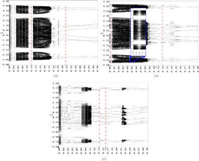
Figure 1:

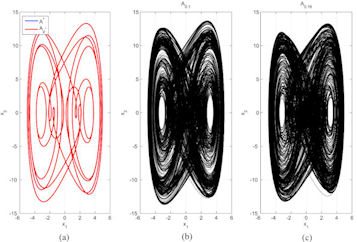
Figure 2:

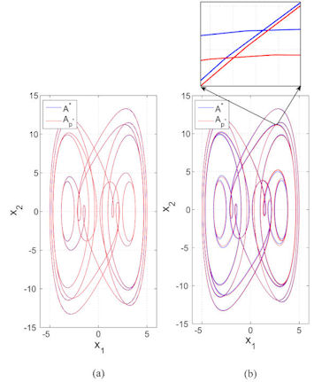
Figure 3:

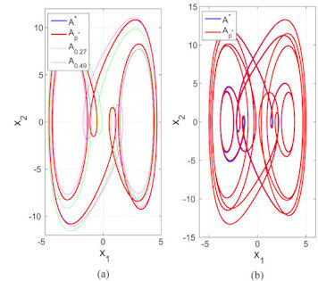
Figure 4:

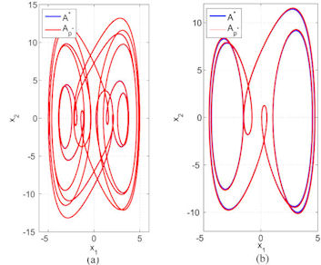
Figure 5:

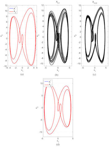
Figure 6:

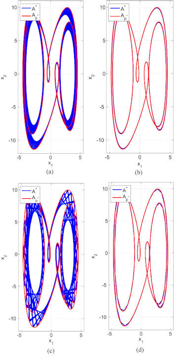
Figure 7:

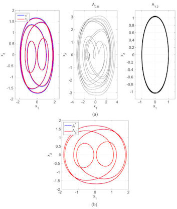
Figure 8:

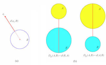
Figure 9:

$$\begin{array}[c]{l}\hline\cr Input:~{}N,~{}P_{N},~{}T,~{}h,~{}m_{1},\ldots,m_{N}\\ t=0\\ Repeat\\ ~{}~{}~{}~{}~{}~{}For~{}k=1~{}to~{}N~{}do\\ \quad~{}~{}~{}\quad~{}~{}~{}~{}p=p_{k}\\ ~{}~{}~{}~{}~{}~{}~{}~{}~{}~{}~{}~{}~{}\,for~{}i=1~{}to~{}m_{k}~{}do\\ ~{}~{}~{}\ ~{}~{}~{}~{}~{}~{}~{}~{}~{}~{}~{}~{}~{}~{}~{}~{}integrate~{}IVP~{}(\ref{ivp generala})\\ ~{}~{}~{}~{}~{}~{}~{}~{}~{}~{}~{}~{}~{}~{}~{}~{}~{}~{}~{}~{}t=t+h\\ ~{}~{}~{}~{}~{}~{}~{}~{}~{}~{}~{}~{}~{}end\\ ~{}~{}~{}~{}~{}~{}~{}end\\ until~{}t\geq T_{\max}\\ \hline\cr\end{array}$$

Table 1:

System	Scheme	$m$	$P_{N}$	$p^{*}$	Fig.
	[$m_{1}p_{1},m_{2}p_{2}]$	$m_{1}=m_{2}=1$	$p_{1}=0.1,~{}p_{2}=0.16$	$0.13$	2
	[$m_{1}p_{1},...,m_{4}p_{4}]$	$m_{1}=m_{4}=2,~{}m_{2}=m_{3}=1$	$\begin{array}[]{c}p_{1}=0.11,~{}p_{2}=0.12,\\ ~{}p_{3}=0.14,~{}p_{4}=0.15\end{array}$	$0.13$	3a
$\begin{array}[]{c}IVP(\ref{cont})\\ c=0\\ d=0\end{array}$	[$m_{1}p_{1},...,m_{21}p_{21}]$	$\begin{array}[]{c}m_{1}=3,~{}m_{2}=m_{4}=4,~{}m_{3}=2,\\ m_{5}=...=m_{8}=1\\ m_{9}=m_{10}=2,\\ m_{11}=...=m_{21}=1\end{array}$	$\begin{array}[]{c}p_{k}=0.05+k\times 0.01,\\ k=0,1,...,21,~{}k\neq 8\end{array}$	$0.13$	3 b
	$[m_{1}p_{1},m_{2}p_{2}]$	$m_{1}=3,~{}m_{2}=1$	$p_{1}=0.27,~{}p_{2}=0.49$	$0.325$	4 a
	random scheme		$p_{1}=0.12,~{}p_{2}=0.14$	$\begin{array}[]{c}p^{o}=0.13001\\ p^{*}=0.13\end{array}$	4 b
	$[m_{1}p_{1},m_{2}p_{2}]$	$\begin{array}[]{c}m_{1}=1,~{}m_{2}=1\\ \end{array}$	$\begin{array}[]{c}p_{1}=0,p_{2}=0.075\end{array}$	$0.0375$	5 a
$\begin{array}[]{c}IVP(\ref{discont1})\\ c=0\\ d=1\end{array}$	[$m_{1}p_{1},...,m_{10}p_{10}]$	$\begin{array}[]{c}m_{1}=...=m_{9}=1,\\ m_{10}=2,\\ \end{array}$	$\begin{array}[]{c}p_{k}=0.05+k\times 0.01,\\ k=1,2,...,11,~{}k\neq 6\end{array}$	$0.12$	5 b
$\begin{array}[]{c}\\ IVP(\ref{discont2})\\ c=1\\ d=0\end{array}$	[$m_{1}p_{1},m_{2}p_{2}]$	$\begin{array}[]{c}m_{1}=1,~{}m_{2}=1\end{array}$	$\begin{array}[]{c}p_{1}=0.04,p_{2}=0.28\end{array}$	$0.16$	6 a
	$[m_{1}p_{1},...,m_{10}p_{10}]$	$\begin{array}[]{c}m_{1}=...=m_{10}=1\\ \end{array}$	$\begin{array}[]{c}p_{k}=(k-1)\times 0.03,\\ k=1,...,10\end{array}$	$0.135$	6 b

Table 2:

Figure captions

Fig. 1. Bifurcation diagram of the Duffing system (3). The dashed lines present the parameter values corresponding to the synthesized attractors. (a) Continuous case ($c=d=0$). (b) Discontinuous case ($c=0,~{}d=1$). (c) Discontinuous case ($c=1,~{}d=0$).

Fig. 2. The PS algorithm applied to the continuous Duffing system (8) with $N=2$, $P_{2}=\{0.1,0.16\}$ and $m_{1}=m_{2}=1$. (a) $A^{*}$ and $A_{p^{*}}$, with $p^{*}=0.13$. (b) Attractor $A_{0.1}$. (c) Attractor $A_{0.16}$.

Fig. 3. The stable limit cycle $A_{0.13}$ of the continuous Duffing system (8) obtained with $\left(a\right)$ $[2p_{1},1p_{2},1p_{3},2p_{4}]$, for $p_{1}=0.11,p_{2}=0.12,p_{3}=0.14,p_{4}=0.15$. (b) Same attractor $A_{0.13}$ for $N=21$ with $p_{k}=0.05+k\times 0.01,k=1,2,...,20,k\neq 8$ and $m_{1}=3,m_{2}=4,m_{3}=2,m_{4}=4,m_{5}=m_{6}=m_{7}=m_{8}=m_{9}=1,m_{10}=m_{11}=2,m_{12}=...=m_{21}=1$. Both attractors $A^{*}$ and $A_{p^{*}}$, with $p^{*}=0.13$, are plotted superimposedly.

Fig. 4. (a) The stable limit cycle $A_{0.325}$ of the continuous Duffing system (8) obtained with $P_{N}=\{0.27,0.49\}$ and the scheme $[3p_{1},1p_{2}\}$. All the attractors, $A^{*}$, $A_{p^{*}}$ (with $p^{*}=0.325$), $A_{0.27}$, and $A_{0.49}$, are plotted in the same phase plane. (b) The PS algorithm applied with uniformly distributed random switching of $p$ within the set $\{0.12,0.14\}$ to obtain the attractor $A_{0.13}$.

Fig. 5. (a) Stable limit cycle $A_{0.0375}$ for the discontinuous Duffing system (9), obtained with $[m_{1}p_{1},m_{2}p_{2}]$ for $p1=0,p2=0.075$ and $m_{1}=m_{2}=1$. b) Stable limit cycle $A_{0.12}$ obtained with the scheme $[m_{1}p_{1},...,m_{10}p_{10}]$, with $p_{k}=k0.01+0.05$, $k=1,...,11$, $k\neq 6$ and $m_{1}=...=m_{9}=1$, $m_{10}$=2.

Fig. 6. Stable limit cycle $A_{0.16}$ of the discontinuous Duffing system (10) obtained with the scheme $[1\times 0.1,1\times 0.22]$. (a) $A^{*}$ and $A_{p^{*}}$ with $p^{*}=0.16$. (b) $A_{0.1}$. (c) $A_{0.22}$. (d) Stable limit cycle $A_{0.135}$ obtained with the scheme $[m_{1}p_{1},m_{2}p_{2},...,m_{10}p_{10}]$ with $p_{k}=(i-1)0.03$, $i=1,2,...,10$ and $m_{k}=1$, $k=1,2,...,10$. $p^{*}=0.135$.

Fig. 7. Stable limit cycle $A_{0.13}$ of the discontinuous Duffing system (9) obtained with $[m_{1}p_{1},m_{2}p_{2}]$ with: (a) $m_{1}=m_{2}=25$ and $h=0.005$. (b) $m_{1}=m_{2}=25$, $h=0.001$. (c) $m_{1}=m_{2}=35$, $h=0.005$. (d) $m_{1}=m_{2}=35$, $h=0.001$.

Fig. 8. (a) The PS algorithm applied to the system (11) for $p=\alpha$ as control parameter and with $N=2$, $P_{N}=\{0.8,1.2\}$ and scheme $[1p_{1},p_{2}]$. (b) The PS algorithm with $N=100$, applied to the same system, but with $p=\xi$.

Fig. 9. Hausdorff hdistance. (a) $d(a_{i},B)$; (b) $D_{H}$ for two ideal cases. A suggested applet can be found from [30].

Table captions

Table 1. Pseudo-code of the PS algorithm.

Table 2. The PS algorithm applied to the Duffing systems (8), (9) and (10).

References

- [1] J.-P. Aubin, A. Cellina, Differential inclusions set-valued maps and viability theory, Springer, Berlin, 1984.
- [2] S. Banerjee, K. Chakrabarty, Nonlinear modeling and bifurcations in the boost converter, IEEE Trans Power Electron, 13 (2) (1998) 252–260.
- [3] N.V. Butenin, Y.I. Nejmark, N.A. Fufaev, An introduction to the theory of nonlinear oscillations (In Russian), Nauka, Moscow, 1987.
- [4] Q. Cao, M. Wiercigroch, E.E. Pavlovskaia, C. Grebogi, J. Michael, T. Thompson, Archetypal oscillator for smooth and discontinuous dynamics, Physical Review E 74 (2006) 046218.
- [5] M.-F. Danca, W.K.S. Tang, G. Chen, A switching scheme for synthesizing attractors of dissipative chaotic systems, Appl. Math. Comput. 201 (1-2) (2008) 650 -667.
- [6] M.-F. Danca, Random parameter-switching synthesis of a class of hyperbolic attractors, Chaos 18 (2008) 033111.
- [7] M.-F. Danca, K. Diethlem, Fractional-order attractors synthesis via parameter switchings, Commun. Nonlinear Sci. Numer. Simulat. 15(12) (2010) 3745 -353.
- [8] M.-F. Danca, M. Romera, G. Pastor, F. Montoya, Finding attractors of continuous-time systems by parameter switching, Nonlinear Dynamics, 67(4) (2012) 2317 -2342.
- [9] K. Deimling, Multivalued differential equations, W. De Gruyter, Berlin, 1992.
- [10] K. Falconer, Fractal geometry, Mathematical foundations and applications, John Wiley & Sons, Chichester, 1990.
- [11] A.F. Filippov, Differential equations with discontinuous right-hand sides, Kluwer Academic, Dordrecht, 1988.
- [12] C. Foias, M.S. Jolly, On the numerical algebraic approximation of global attractors, Nonlinearity 8 (1995) 295–319.
- [13] J. Guckenheimer, P. Holmes, Nonlinear oscillations, dynamical systems, and bifurcations of vector fields (Applied Mathematical Sciences Vol. 42), Springer-Verlag, New York, 1983.
- [14] J.L. Kaplan, J.A. Yorke, Preturbulence: a regime observed in a fluid flow model of Lorenz, Commun. Math. Phys. 67(2) (1979) 93–108.
- [15] M. Kunze, T. Küpper, Qualitative bifurcation analysis of a non-smooth friction-oscillator model, Z. Angew. Math. Phys. 48(1) (1997) 87–101.
- [16] M. Kunze, Non-smooth dynamical systems, Springer, Berlin, 2000.
- [17] Y. Mao, W.K.S. Tang, M.-F. Danca, An averaging model for the chaotic system with periodic time-varying parameter, Appl. Math. Comput. 217(1) (2010) 355–362.
- [18] M.-F. Danca, Convergence of a parameter switching algorithm for a class of nonlinear continuous systems and a generalization of Parrondo’s paradox, Comm. Non. Sci. Num. Sim. 18(3), (2013) 500- 510.
- [19] F.C. Moon, P.J. Holmes, A magnetoelastic strange attractor, J. Sound Vibration 65 (2) (1979) 275-296.
- [20] U. Parlitz, W. Lauterborn, Superstructure in the bifurcation set of the Düffing equation , Phys. Lett. 107A (8) (1985) 351–355.
- [21] A. Polynikis, S.J. Hogan, M. di Bernardo, Comparing different ODE modelling approaches for gene regulatory networks, J Theor. Biol. 261(4) (2009) 511–530.
- [22] E.P. Popov, The dynamics of automatic control systems (Translated from the Russian), Pergamon, Oxford, 1962.
- [23] K, Popp, N. Hinrichs, M. Oestreich, Dynamical behaviour of a friction oscillator with simultaneous self and external excitation, S adhan a 20,(2-4) (1995) 627–654.
- [24] K. Popp, P. Stelter, Stick-slip vibrations and chaos, Philos Trans R Soc London A 332 (1990) 89–105.
- [25] J.A. Sanders, F. Verhulst, Averaging methods in nonlinear dynamical systems, Springer-Verlag, New York, 1985.
- [26] J.J. Slotine, S.S. Sastry, Tracking control of nonlinear systems using sliding surfaces with application to robot manipulators. Int J Control 38 (2) (1983) 465–492.
- [27] A. Stuart, A.R. Humphries, Dynamical systems and numerical analysis, Cambridge Monographs on Applied and Computational Mathematics (No. 2), Cambridge University Press, Cambridge, 1998.
- [28] Y. Ueda, Random phenomena resulting from nonlinearity in the system described by Duffing s Equation, Int. J. Non-Linear Mechanics 20 (5-6) (1985) 481–491.
- [29] M. Wiercigroch, B. de Kraker, Applied nonlinear dynamics and chaos of mechanical systems with discontinuities, World Scientific, Singaporem, 2000.
- [30] http://faculty.gvsu.edu/schlicks/HausdorffGeometry/H2.htm.