Blanchfield forms and Gordian distance

Abstract.

Given a link in $S^{3}$ we will use invariants derived from the Alexander module and the Blanchfield pairing to obtain lower bounds on the Gordian distance between links, the unlinking number and various splitting numbers. These lower bounds generalise results recently obtained by Kawauchi.

We give an application restricting the knot types which can arise from a sequence of splitting operations on a link. This allows us to answer a question asked by Colin Adams in 1996.

1. Introduction

1.1. Lower bounds on the clasp number and the Gordian distance

In this paper, by an $m$-component link $L\subset S^{3}$ we mean an embedding

$$L\colon\cup_{i=1}^{m}S^{1}\times\{i\}\to S^{3}.$$

Given $i=1,\dots,m$ we write $L_{i}=L(S^{1}\times\{i\})$ and we endow it with the orientation inherited from the standard orientation of $S^{1}$. By a slight abuse of notation we often denote the union of the $L_{i}$ again by $L$. Throughout the paper we will identify two $m$-component links $L$ and $J$ if there exists an isotopy through links from $L$ to $J$. Slightly more informally, an $m$-component link is an isotopy class of an oriented, ordered collection of $m$ disjoint circles in $S^{3}$.

Let $L$ and $J$ be $m$-component links in $S^{3}$. We are interested in the following measures of how different $L$ and $J$ are.

1. The Gordian distance $g(L,J)$ which is defined as the minimal number of crossing changes required to turn a diagram representing $L$ into a diagram for $J$. Here we take the minimum over all diagrams of $L$.

2. The 4-dimensional clasp number $c(L,J)$ which is the minimal number of double points of an immersed concordance between $L$ and $J$. An immersed concordance is a proper immersion of $m$ annuli $f_{j}\colon S^{1}\times I\looparrowright S^{3}\times I$ with $f_{j}(S^{1}\times\{0\})=L_{j}\times\{0\}$ and $f_{j}(S^{1}\times\{1\})=-J_{j}\times\{1\}$, for $j=1,\dots,m$. The only allowed singularities of the immersion are ordinary double points.

Note that $c(L,J)\leq g(L,J)$ since a sequence of crossing changes and isotopies gives rise to an immersed concordance, with one double point for each crossing change.

Our goal in this paper is to give lower bounds on the Gordian distance and the 4-dimensional clasp number from the Alexander module and the Blanchfield pairing of a link. The relationship between the Alexander module and the unlinking number has been explored in several earlier papers, see e.g. [BW84, Tra88, CFP13]. The first and second authors undertook a systematic study of the relationship between the Blanchfield pairing and the unknotting number of knots in [BF12, BF13].

Given an $m$-component link $L$ we refer to the complement of an open tubular neighbourhood of $L$ as the exterior of $L$ and we denote it by $X_{L}=S^{3}\setminus\nu L$. We write $\Lambda=\mathbb{Z}[t_{1}^{\pm 1},\dots,t_{m}^{\pm 1}]$. We can associate the Alexander module $H_{1}(X_{L};\Lambda)$ to $L$ and we denote the rank of the Alexander module by $\beta(L):=\operatorname{rank}_{\Lambda}(H_{1}(X_{L};\Lambda))$. The Alexander polynomial $\Delta_{L}\in\Lambda$ of $L$ is defined as the order of the Alexander module. Note that $\Delta_{L}=0$ if and only if $\beta(L)>0$. We also consider the torsion Alexander polynomial $\Delta^{\operatorname{tor}}_{L}$ as the order of the torsion submodule $\operatorname{Tor}_{\Lambda}H_{1}(X_{L};\Lambda)$. Note that $\Delta^{\operatorname{tor}}_{L}$ is always non-zero.

Next we consider the Blanchfield form, which was first introduced for knots by Blanchfield [Bl57] in 1957. Let $S\subset\Lambda$ be the multiplicative subset generated by the polynomials $t_{i}-1$, for $i=1,\dots,m$. By inverting the elements of $S$ we obtain the ring

$$\Lambda_{S}:=\mathbb{Z}[t_{1}^{\pm 1},\dots,t_{m}^{\pm 1},(t_{1}-1)^{-1},\dots,(t_{m}-1)^{-1}].$$

Furthermore we denote the quotient field of $\Lambda$ by $\Omega=\mathbb{Q}(t_{1},\dots,t_{m})$. This is also the quotient field of $\Lambda_{S}$. The Blanchfield form

$$\operatorname{Bl}_{L}\colon\hat{t}H_{1}(X_{L};\Lambda_{S})\times\hat{t}H_{1}(X_{L};\Lambda_{S})\to\Omega/\Lambda_{S}$$

is a nonsingular, hermitian, sesquilinear form defined on a certain quotient $\hat{t}H_{1}(X_{L};\Lambda_{S})$ of the torsion submodule $\operatorname{Tor}_{\Lambda_{S}}H_{1}(X_{L};\Lambda_{S})$; see Section 2 for details. We say that a hermitian form $\lambda\colon H\times H\to\Omega/\Lambda_{S}$ is metabolic if it admits a metabolizer, i.e. a submodule $P$ of $H$ with $P=P^{\perp}:=\{h\in H\,|\,\lambda(p,h)=0\mbox{ for all }p\in P\}$. The following is our first main theorem.

Theorem 1.1.

Let $L$ and $J$ be $m$-component links. Then $|\beta(L)-\beta(J)|\leq c(L,J)$. Moreover, if $c(L,J)=|\beta(L)-\beta(J)|$, then the Witt sum of Blanchfield forms $\operatorname{Bl}_{L}\oplus-\operatorname{Bl}_{J}$ is metabolic.

In the following, given $f=f(t_{1},\dots,t_{m})\in\Lambda$ we write $\overline{f}:=f(t_{1}^{-1},\dots,t_{m}^{-1})$. Furthermore, we say that a polynomial $n\in\Lambda$ is negligible if it is of the form

$$n=\pm\prod_{i=1}^{m}t_{i}^{r_{i}}\,\,\cdot\,\prod_{i=1}^{m}(1-t_{i})^{s_{i}}$$

where $r_{i},s_{i}\in\mathbb{Z}$ for $i=1,\dots,m$; this is equivalent to saying that $n$ is invertible in $\Lambda_{S}$. We can formulate the following straightforward corollary to Theorem 1.1.

Corollary 1.2.

Let $L$ and $J$ be $m$-component links. If $c(L,J)=|\beta(L)-\beta(J)|$, then $\Delta^{\operatorname{tor}}_{L}\cdot f\,\overline{f}=\Delta^{\operatorname{tor}}_{J}\cdot g\,\overline{g}\cdot n$ for some non-zero $f,g\in\Lambda$ and some negligible $n\in\Lambda$.

The inequality $|\beta(L)-\beta(J)|\leq c(L,J)$ in Theorem 1.1 and the statement of the corollary are essentially the main result of a recent paper by Kawauchi [Ka13]. (Kawauchi gives a slightly more precise version of the corollary in so far as he also determines the negligible element $n$.) In the case of single variable Alexander modules, the rank estimate was previously given by Kawauchi in [Ka96]. The result on Blanchfield forms is to the best of our knowledge a new result.

Our second main theorem gives a refinement of Corollary 1.2 when we replace the clasp number by the Gordian distance. More precisely we have the following theorem.

Theorem 1.3.

Let $L$ and $J$ be two $m$-component links. Then

$$|\beta(L)-\beta(J)|\leq g(L,J).$$

Furthermore, if $\beta(J)=\beta(L)+g(L,J)$, then

$$\Delta^{\operatorname{tor}}_{L}=\Delta^{\operatorname{tor}}_{J}\cdot f\,\overline{f}\cdot n$$

for some $f\in\Lambda$ and some negligible $n\in\Lambda$.

Put differently, since Gordian distance is more specialized than 4-dimensional clasp number, we are able to show that one torsion polynomial divides the other.

1.2. The splitting number and the weak splitting number

We now recall and introduce a few more link theoretic notions.

1. The unlinking number $u(L)$ of an $m$-component link $L$ is the Gordian distance to the $m$-component unlink.

2. An $m$-component link $L$ is a split link if there are $m$ disjoint balls in $S^{3}$ each of which contains a component of $L$.

3. Following [BS13, CFP13], the splitting number $\operatorname{sp}(L)$ of a link $L$ is the minimal number of crossing changes between different components of $L$ required on some diagram of $L$ to obtain a split link, where the minimum is taken over all diagrams.

4. The weak splitting number $\operatorname{wsp}(L)$ of a link $L$ is the minimal number of crossing changes required on some diagram of $L$ to produce a split link, where the minimum is taken over all diagrams.

Note that for the weak splitting number, unlike the splitting number considered above, crossing changes of a component with itself are permitted. For example if $L$ is the Whitehead link then it is straightforward to see that $\operatorname{wsp}(L)=1$, but an elementary linking number argument (see [CFP13, Section 2]) shows that $\operatorname{sp}(L)=2$. Somewhat confusingly the weak splitting number is referred to as the splitting number in [Ad96, Sh12, La14], but we decided to follow the convention used by Batson–Seed [BS13].

It is straightforward to apply Theorem 1.3 to the computation of unlinking numbers, splitting numbers and weak splitting numbers. The precise statements are given in Corollaries 4.2, 4.3 and 4.4. We note that the result on splitting numbers, Corollary 4.3, considerably strengthens [CFP13, Theorem 4.2].

In Section 5 we give some examples of the use of these corollaries. Corollary 4.2 enables us to easily compute the unlinking numbers of the 3-component links with 9 or fewer crossings. We also show that some, but not all, of the results on splitting numbers from [CFP13] which were obtained using covering links, can also be obtained with the algebraic methods of this paper.

1.3. Knot types from weak splitting operations

Now we turn to an application of Theorems 1.1 and 1.3 to weak splitting numbers. Let us introduce some notation. If a link $J$ can be obtained from a link $L$ by a sequence of $r$ crossing changes then we write $L\rightsquigarrow_{r}J$. A sequence of crossing changes culminating in a split link is referred to as a splitting sequence. Given knots $K_{1},\dots,K_{m}$ we denote the split link comprising these knots by $K_{1}\sqcup\dots\sqcup K_{m}$. We write $U$ for the unknot throughout this subsection.

In Section 6 we give a general condition in terms of Blanchfield forms and Alexander polynomials restricting the knot types which can arise from a sequence of crossing changes realising the weak splitting number; see Theorem 6.1.

In [Ad96] Adams gave some examples of 2-component links $L$ with unknotted components and $\operatorname{wsp}(L)=1$, such that whenever one turns $L$ into a split link using a single crossing change, the resulting split link has a knotted component. Put differently, for the given link $L$ one has to pay a price for splitting it with one crossing change, i.e. one has to turn one of the unknotted components into a non-trivial knot.

Adams then asked whether there are occasions when the price to pay must be ‘arbitrarily high’. More precisely, the following question was asked by Adams [Ad96, p. 299].

Question 1.4.

Let $C$ be a complexity for knots, e.g. crossing number, hyperbolic volume, span of some knot polynomial. Given any $c\in\mathbb{N}$, does there exist a $2$-component link $L$ with unknotted components such that for any splitting sequence $L\rightsquigarrow_{1}K\sqcup U$ of length one we have $C(K)\geq c$?

We give an affirmative answer to Adams’ question for the crossing number.

Theorem 1.5.

Fix $c\in\mathbb{N}$. There exists a 2-component link $L$ with unknotted components such that such for any knot $K$ with $L\rightsquigarrow_{1}K\sqcup U$, the crossing number of $K$ is at least $c$.

Next we give a quick summary of the proof of Theorem 1.5. Given $c\in\mathbb{N}$ we combine constructions from [Ad96] and [Kon79] to obtain a link $L$ with $L\rightsquigarrow_{1}J\sqcup U$ where $J$ is a knot such that the degree of $\Delta_{J}(t)$ is $2n$ and $\Delta_{J}$ is irreducible, chosen so that $n$ is suitably high with respect to $c$. Then we find that for any $K$ as in Theorem 1.5, we have $\Delta_{J}|\Delta_{K}$, so that the degree of $\Delta_{K}$ is forced to be at least $2n$. The theorem follows since the degree of the Alexander polynomial gives a lower bound on the crossing number.

In fact, it is straightforward to modify the proof of Theorem 1.5 to give an affirmative answer to Adams’ question for the support of knot Floer homology and the 3-genus as the complexity, since the Alexander polynomial provides a lower bound for these as well.

The paper is organized as follows. In Section 2 we recall the definitions and basic properties of the Alexander module and the Blanchfield form of a link. In Section 3 we provide the proof of Theorem 1.1 and Corollary 1.2. In Section 4 we will prove Theorem 1.3 and we will state several corollaries relating Alexander polynomials to the unlinking number, the splitting number and the weak splitting number of a link. In Section 5 we give examples of unlinking and splitting number computations. In Section 6 we investigate weak splitting numbers and the knot types arising from them; in particular we give the proof of Theorem 1.5.

Conventions.

All rings are commutative and all modules are finitely generated. Links are oriented and ordered.

Acknowledgment.

Work on this paper was supported by the SFB 1085 ‘Higher Invariants’ at the Universität Regensburg funded by the DFG. This paper has roots in joint work of two of us with Jae Choon Cha, and we wish to thank him, and also Patrick Orson, for many helpful conversations. We would also like to thank Lorenzo Traldi for helpful comments on the first version of the article.

2. The Alexander module and the Blanchfield form

2.1. Alexander modules

Throughout the paper we identify the group ring of $\mathbb{Z}^{m}$ with the multivariable Laurent polynomial ring $\Lambda:=\mathbb{Z}[t_{1}^{\pm 1},\dots,t_{m}^{\pm 1}]$ in the canonical way. (We suppress $m$ from the notation, but it will always be clear from the context which $m$ we mean.) We denote by $f\mapsto\overline{f}$ the involution on $\Lambda$ which is given by the unique $\mathbb{Z}$-linear ring homomorphism with $t_{i}\mapsto t_{i}^{-1}$, $i=1,\dots,m$. Furthermore, given a $\Lambda$-module $V$ we denote the $\Lambda$-module with involuted $\Lambda$-module structure by $\overline{V}$, i.e. the underlying additive group of $\overline{V}$ is the same as for $V$, but the action of $f$ on $\overline{V}$ is defined as the action of $\overline{f}$ on $V$.

Throughout the paper we will mostly be interested in the following $\Lambda$-modules:

1. the ring $\Lambda$ itself,

2. the ring $\Lambda_{S}:=\mathbb{Z}[t_{1}^{\pm 1},\dots,t_{m}^{\pm 1},(t_{1}-1)^{-1},\dots,(t_{m}-1)^{-1}]$, which is the multivariable Laurent polynomial ring with the monomials $t_{i}-1$ inverted,

3. the quotient field $\Omega$ of $\Lambda$, which is also the quotient field of $\Lambda_{S}$.

In the following let $X$ be a connected manifold and let $\varphi\colon\pi_{1}(X)\to\mathbb{Z}^{m}$ be a homomorphism. We denote the cover corresponding to $\varphi$ by $p\colon\widetilde{X}\to X$. Given $Y\subset X$ we write $\widetilde{Y}:=p^{-1}(Y)$. Note that the group $\mathbb{Z}^{m}$ acts by deck transformations on $C_{*}(\widetilde{X},\widetilde{Y})$ on the left. Thus we can view $C_{*}(\widetilde{X},\widetilde{Y})$ as a (left) $\mathbb{Z}[\mathbb{Z}^{m}]=\Lambda$-module. Now let $M$ be a (left) $\Lambda$-module. Then we consider the following (right) $\Lambda$-modules:

$$\begin{array}[]{rcl}H_{i}(X,Y;M)&:=&H_{i}\left(\overline{C_{*}(\widetilde{X},\widetilde{Y})}\otimes_{\Lambda}M\right),\mbox{ and }\\[5.69054pt] H^{i}(X,Y;M)&:=&H_{i}\left(\operatorname{Hom}_{\Lambda}(C_{*}(\widetilde{X},\widetilde{Y}),M)\right).\end{array}$$

As usual we write $H_{i}(X;M)=H_{i}(X,\emptyset;M)$ and $H^{i}(X;M)=H^{i}(X,\emptyset;M)$.

Now let $L$ be an $m$-component link. We denote the exterior of $L$ by $X_{L}$. Note that $\pi_{1}(X_{L})$ admits a canonical epimorphism $\phi_{L}$ onto $\mathbb{Z}^{m}$ which is given by sending the $i$-th oriented meridian to the $i$-th vector of the standard basis of $\mathbb{Z}^{m}$. In the following we will refer to $H_{1}(X_{L};\Lambda)$ as the Alexander module of $L$.

We recall several basic properties of twisted homology and cohomology groups. The following lemma is well-known; see e.g. [HS71, Section VI.3].

Lemma 2.1.

Let $X$ be a connected CW-complex and let $\varphi\colon\pi_{1}(X)\to\mathbb{Z}^{m}$ be a homomorphism. Then for any $\Lambda$-module $M$ we have

$$H_{0}(X;M)\cong M/\Big{\{}\sum_{i=1}^{m}\varphi(g_{i})v_{i}-v_{i}\,|\,v_{1},\dots,v_{m}\in M\mbox{ and }g_{1},\dots,g_{m}\in\pi_{1}(X)\Big{\}}.$$

In particular, if $M$ is a field and $\varphi$ is non-trivial, then $H_{0}(X;M)=0$.

The following theorem is a well-known instance of Poincaré duality and the Universal Coefficient Theorem.

Theorem 2.2.

Let $X$ be a connected oriented $k$-manifold and let $\varphi\colon\pi_{1}(X)\to\mathbb{Z}^{m}$ be a homomorphism. Let $\partial X=Y_{0}\cup Y_{1}$ be a decomposition of the boundary into two submanifolds with $\partial Y_{0}=\partial Y_{1}$. Then for any $\Lambda$-module $M$ we have an isomorphism

$$\operatorname{PD}\colon H_{i}(X,\partial Y_{0};M)\xrightarrow{\cong}\overline{H^{k-i}(X,\partial Y_{1};M)}.$$

In particular, if $M=\Omega$ is the quotient field of $\Lambda$, then $H_{i}(X,\partial Y_{0};\Omega)\cong H_{k-i}(X,\partial Y_{1};\Omega)$.

2.2. Ranks and orders of modules

Let $R$ be a domain with quotient field $Q$. Let $M$ be an $R$-module. We then refer to $\operatorname{rank}_{R}(M):=\dim_{Q}(M\otimes_{R}Q)$ as the rank of $M$. Now suppose that $R$ is in fact a UFD and that $M$ is finitely generated. We pick a resolution

$$R^{k}\xrightarrow{A}R^{\,l}\to M\to 0$$

with $k\in\mathbb{N}\cup\{\infty\}$. After adding possibly columns of zeros we can and will assume that $k\geq l$. The order $\operatorname{ord}(A)$ of $M$ is defined as the greatest common divisor of the $l\times l$-minors of $A$. Note that the order is well-defined up to multiplication by a unit in $R$; see [CF77] for details. Also note that $\operatorname{ord}(A)\neq 0$ if and only if $\operatorname{rank}(A)=0$.

For future reference we record the following lemma. A proof can be found in [Hi12, Chapter 3.3].

Lemma 2.3.

Let $R$ be a UFD and let

$$0\to A\to B\to C\to 0$$

be a short exact sequence of finitely generated $R$-modules. Then

$$\operatorname{ord}(B)=\operatorname{ord}(A)\cdot\operatorname{ord}(C).$$

In the following, given $f,g\in R$ we write $f\doteq g$ if $f=ug$ for some unit $u\in R$. We will mostly be interested in the rings $R=\Lambda$ and $R=\Lambda_{S}$. Note that the units in $\Lambda=\mathbb{Z}[t_{1}^{\pm 1},\dots,t_{m}^{\pm 1}]$ are precisely the monomials $\pm t_{1}^{n_{1}}\dots t_{m}^{n_{m}}$. Furthermore, the units in

$$\Lambda_{S}=\mathbb{Z}[t_{1}^{\pm 1},\dots,t_{m}^{\pm 1},(t_{1}-1)^{-1},\dots,(t_{m}-1)^{-1}]$$

are precisely the products of monomials and powers of $t_{i}-1$, $i=1,\dots,m$. Put differently, the units in $\Lambda_{S}$ are the negligible elements from the introduction.

Given an $m$-component link $L$ we write

$$\beta(L):=\operatorname{rank}_{\Lambda}(H_{1}(X_{L};\Lambda)).$$

Note that $X_{L}$ is compact, so in particular $X_{L}$ is homeomorphic to a finite CW-complex, which in turn implies that the cellular chain complex $C_{*}(\widetilde{X_{L}})$ is finitely generated over $\Lambda$. Since $\Lambda$ is Noetherian it follows that $H_{1}(X_{L};\Lambda)$ and $\operatorname{Tor}_{\Lambda}H_{1}(X_{L};\Lambda)$ are finitely generated $\Lambda$-modules. We refer to

$$\Delta_{L}:=\operatorname{ord}(H_{1}(X_{L};\Lambda))$$

as the Alexander polynomial of $L$. Furthermore, we refer to

$$\Delta^{\operatorname{tor}}_{L}:=\operatorname{ord}(\operatorname{Tor}_{\Lambda}H_{1}(X_{L};\Lambda))$$

as the torsion Alexander polynomial of $L$.

Recall that an $m$-component link is split if there exist $m$ disjoint 3-balls in $S^{3}$, each of which contains a component of $L$. Later on we will need the following well-known lemma.

Lemma 2.4.

Let $L$ be a split $m$-component link. Then $\beta(L)=m-1$ and $\Delta^{\operatorname{tor}}_{L}\doteq\Delta_{L_{1}}(t_{1})\cdot\ldots\cdot\Delta_{L_{m}}(t_{m})$.

Proof.

We just provide a short sketch of the well-known proof. By our hypothesis there exist disjoint balls $B_{1},\dots,B_{m}$ in $S^{3}$, such that $L_{i}\subset B_{i}$, $i=1,\dots,m$. We write $S_{i}=\partial B_{i}$, $i=1,\dots,m$ and $C:=\overline{S^{3}\setminus\cup_{i=1}^{m}B_{i}}$.

Note that $H_{1}(S_{i};\Lambda)=H_{1}(C;\Lambda)=0$ and $H_{0}(S_{i};\Lambda)=H_{0}(C;\Lambda)=\Lambda$. Also, a straightforward argument shows that for $j=0,1$ and $i\in\{1,\dots,m\}$ we have

$$H_{j}(B_{i}\setminus\nu L_{i})\cong H_{j}(S^{3}\setminus\nu L_{i};\Lambda)\cong H_{j}(S^{3}\setminus\nu L_{i};\mathbb{Z}[t_{i}^{\pm 1}])\otimes_{\mathbb{Z}[t_{i}^{\pm 1}]}\Lambda.$$

It follows easily from Lemma 2.1 that $H_{0}(S^{3}\setminus\nu L_{i};\mathbb{Z}[t_{i}^{\pm 1}])\cong\mathbb{Z}[t_{i}^{\pm 1}]/(t_{i}-1)\mathbb{Z}[t_{i}^{\pm 1}]$. Furthermore it follows from the definitions that $M_{i}:=H_{1}(S^{3}\setminus\nu L_{i};\mathbb{Z}[t_{i}^{\pm 1}])$ is a module whose order equals $\Delta_{L_{i}}(t_{i})$.

The Mayer–Vietoris sequence with $\Lambda$ coefficients corresponding to the decomposition $S^{3}\setminus\nu L=\bigcup_{i=1}^{m}(B_{i}\setminus\nu L_{i})\,\cup\,C$ gives rise to the following exact sequence:

By Lemma 2.1 the module $H_{0}(S^{3}\setminus\nu L;\Lambda)$ is $\Lambda$-torsion. The lemma now follows immediately from the above observations and from elementary properties of ranks and orders. We leave the details to the reader. ∎

2.3. The maximal pseudo-null submodule

Given a ring $R$ and a module $M$ over $R$ we denote the torsion submodule by $TM$. Furthermore we denote the maximal pseudo-null submodule of $M$ by $zM$; this is the submodule of $TM$ which is generated by the elements of $M$ whose annihilator is not contained in any principal ideal of $R$. Following [Hi12, Section 2.3] we write

$$\hat{t}M:=TM/zM.$$

For future reference we record the following lemma, see [Hi12, Theorem 3.5].

Lemma 2.5.

For any $\Lambda$-module $M$ we have $\operatorname{ord}(TM)=\operatorname{ord}(\hat{t}M)$.

2.4. Linking forms

Let $R$ be a ring with (possibly trivial) involution. We denote the quotient field of $R$ by $Q$. Here and throughout the paper we extend the involution on $R$ to an involution on $Q$. Let $\lambda\colon H\times H\to Q/R$ be a map.

• We say $\lambda$ is sesquilinear if $\lambda(au+bv,w)=\overline{a}\lambda(u,w)+\overline{b}\lambda(v,w)$ and $\lambda(u,av+bw)=\lambda(u,v)a+\lambda(u,w)b$ for all $a,b\in R$ and $u,v,w\in H$.

• We say $\lambda$ is hermitian if $\lambda(u,v)=\overline{\lambda(v,u)}$ for all $u,v\in H$.

• We say that $\lambda$ is nonsingular if the assignment $u\mapsto(v\mapsto\lambda(u,v))$ defines an isomorphism of $R$-modules $\overline{H}\to\operatorname{Hom}(H,Q/R)$.

• A linking form over $R$ is an $R$-module $H$ together with a hermitian sesquilinear nonsingular form $\lambda\colon H\times H\to Q/R$.

• We say that two linking forms $\lambda\colon H\times H\to Q/R$ and $\mu\colon G\times G\to Q/R$ are isomorphic if there is an isomorphism of $R$ modules $f\colon H\xrightarrow{\simeq}G$ such that $\lambda(v,w)=\mu(f(v),f(w))$ for all $v,w\in H$.

• We say that the linking form $\lambda$ is metabolic if $\lambda$ admits a metabolizer, i.e. a submodule $P$ of $H$ with $P=P^{\perp}:=\{v\in H\,|\,\lambda(p,v)=0\mbox{ for all }p\in P\}$.

• Given a linking form $\lambda\colon H\times H\to Q/R$ we write $-\lambda\colon H\times H\to Q/R$ for the linking form which is defined by $(-\lambda)(v,w)=-\lambda(v,w)$ for all $v,w\in H$.

• Given two linking forms $\lambda\colon H\times H\to Q/R$ and $\lambda^{\prime}\colon H^{\prime}\times H^{\prime}\to Q/R$ we refer to

  $$\begin{array}[]{rcl}\lambda\oplus\lambda^{\prime}\colon(H\oplus H^{\prime})\times(H\oplus H^{\prime})&\to&Q/R\\ ((v\oplus v^{\prime}),(w\oplus w^{\prime}))&\mapsto&\lambda(v,w)+\lambda^{\prime}(v^{\prime},w^{\prime})\end{array}$$

  as the Witt sum of $\lambda$ and $\lambda^{\prime}$.

• We say that two linking forms $(H,\lambda)$ and $(G,\mu)$ are Witt equivalent, written as $(H,\lambda)\sim(G,\mu)$, if there exist metabolic forms $(P,\varphi)$ and $(Q,\phi)$ such that

  $$(H,\lambda)\oplus(P,\varphi)\cong(G,\mu)\oplus(Q,\phi).$$

• The Witt group of linking forms over $R$ is defined as the set of Witt equivalence classes of linking forms. The identity element of the Witt group is the equivalence class of the linking form on the zero module and the inverse of $[(H,\lambda)]$ is given by $[(H,-\lambda)]$.

For the record we state the following well-known lemma which is proved in [Hi12, Lemma 3.26], for example.

Lemma 2.6.

Let $R$ be a UFD with (possibly trivial) involution. If $\lambda\colon H\times H\to Q/R$ is a metabolic linking form, then $\operatorname{ord}(H)\doteq f\cdot\overline{f}$ for some $f\in R$.

2.5. The Blanchfield form

In this section we sketch the definition of Blanchfield forms for 3-manifolds and we summarize a few key properties. We refer to [Hi12, Section 2] for a thorough treatment of Blanchfield forms.

Let $N$ be a $3$-manifold (with possibly nonempty boundary) and let $\varphi\colon\pi_{1}(N)\to\mathbb{Z}^{m}$ be a homomorphism, which induces a homomorphism $\mathbb{Z}[\pi_{1}(N)]\to\mathbb{Z}[\mathbb{Z}^{m}]=\Lambda$. Recall that $\Omega$ is the quotient field of $\Lambda$. Let $R$ be a subring of $\Omega$ that contains $\Lambda$ and that is closed under involution. We denote the composition of the following sequence of $R$-module homomorphisms by $\Phi$:

$$\begin{array}[]{rcl}\overline{TH_{1}(N;R)}\xrightarrow{(1)}\overline{TH_{1}(N,\partial N;R)}&\xrightarrow{(2)}&TH^{2}(N;R)\\ &\xrightarrow{(3)}&\operatorname{Ext}^{1}_{R}(H_{1}(N;R),R)\\ &\xrightarrow{(4)}&\operatorname{Ext}^{1}_{R}(TH_{1}(N;R),R)\\ &\xrightarrow{(5)}&\operatorname{Hom}_{R}(TH_{1}(N;R),\Omega/R).\end{array}$$

Here we used the following maps:

1. the inclusion induced map;

2. the Poincaré duality given in Theorem 2.2;

3. the Universal Coefficient Spectral Sequence (see [Hi12, Section 2.1 and 2.4]) gives rise to a pair of exact sequences as in the following diagram, where $V$ is some $R$-module.

   Since $\operatorname{Ext}^{0}_{R}(H_{2}(N,R),R)=\operatorname{Hom}_{R}(H_{2}(N,R),R)$ is torsion-free we obtain a map $TH^{2}(N;R)\to V$, which we then compose with the map

   $$V\to\ker\left(\operatorname{Ext}^{1}_{R}(H_{1}(N,R),R)\to\operatorname{Ext}^{3}_{R}(H_{0}(N,R),R)\right)\,\hookrightarrow\,\operatorname{Ext}^{1}_{R}(H_{1}(N,R),R).$$

4. The map induced by the restriction from $H_{1}(N;R)$ to $TH_{1}(N;R)$.

5. The Bockstein long exact sequence arising from the short exact sequence of coefficients $0\to R\to\Omega\to\Omega/R\to 0$:

   has first and last terms vanishing, the first since $TH_{1}(N;R)$ is $R$-torsion and the last since $\Omega$ is an injective $R$-module. Thus there is a canonical map $\operatorname{Ext}^{1}_{R}(TH_{1}(N;R),R)\to\operatorname{Ext}^{0}_{R}(TH_{1}(N;R),\Omega/R)=\operatorname{Hom}_{R}(TH_{1}(N;R),\Omega/R)$.

Hillman [Hi12, Chapter 2] shows that if $H_{i}(\partial N;R)=0$ for $i=0,1$ and $R$ contains $\Lambda_{S}$, then the resulting map

$$\begin{array}[]{rcl}TH_{1}(N;R)\times TH_{1}(N;R)&\to&\Omega/R\\ (x,y)&\mapsto&\Phi(x)(y)\end{array}$$

descends to a linking form

$$\operatorname{Bl}_{N}\colon\hat{t}H_{1}(N;R)\times\hat{t}H_{1}(N;R)\to\Omega/R$$

that we refer to as the $R$-Blanchfield form of $N$.

Later on we will make use of the following proposition that is proved on [Hi12, p. 40]. (See also [Let00, Proposition 2.8].)

Proposition 2.7.

Let $N$ be a closed $3$-manifold and let $\varphi\colon\pi_{1}(N)\to\mathbb{Z}^{m}$ be a homomorphism. Let $R$ be a subring of $\Omega$ which contains $\Lambda_{S}$. Suppose that there exists a $4$-manifold $W$ with $\partial W=N$ such that $\varphi$ extends over $\pi_{1}(W)$. We write

$$P:=\operatorname{Im}\left\{TH_{2}(W,N;R)\xrightarrow{\partial}TH_{1}(N;R)\to\hat{t}H_{1}(N;R)\right\}.$$

If the sequence

$$TH_{2}(W,N;R)\xrightarrow{\partial}TH_{1}(N;R)\to TH_{1}(W;R)$$

is exact, then $P^{\perp}$ is a metabolizer for the $R$-Blanchfield pairing of $N$.

The proof of this is contained in the proof of [Hi12, Theorem 2.4]. However the situation of his Theorem 2.4 is different to ours, in that the 4-manifold $Z$ in [Hi12] is the exterior of a concordance between two links. Nevertheless the part of his proof on page 40, verbatim except for $(Z,\partial Z)$ replaced with $(W,N)$, provides a proof of Proposition 2.7. There was a slight problem with this part of the proof in the first edition of Hillman’s book, therefore the reader is advised to consult the second edition. A more detailed version of the proof is also given in [Kim14, Section 5.1].

Now let $L$ be an $m$-component link. It is straightforward to see that $H_{*}(\partial X_{L};\Lambda_{S})=0$. We then refer to

$$\operatorname{Bl}_{L}:=\operatorname{Bl}_{X_{L}}\colon\hat{t}H_{1}(X_{L};\Lambda_{S})\times\hat{t}H_{1}(X_{L};\Lambda_{S})\to\Omega/\Lambda_{S}$$

as the Blanchfield form of $L$. Given an $m$-component link $L$ we denote by $\operatorname{Bl}_{L_{i}}(t_{i})$ the linking form which is given by tensoring the Blanchfield form of the knot $L_{i}$ over the ring $\mathbb{Z}[t_{i}^{\pm 1}]$ up to the ring $\Lambda_{S}$. Now we can formulate the following well-known lemma, which can be viewed as a generalization of Lemma 2.4.

Lemma 2.8.

Let $L$ be a split $m$-component link. Then $\beta(L)=m-1$ and $\operatorname{Bl}_{L}\sim\operatorname{Bl}_{L_{1}}(t_{1})\oplus\ldots\oplus\operatorname{Bl}_{L_{m}}(t_{m})$.

Proof.

We only provide a sketch of the proof. The proof of Lemma 2.4 shows that the torsion part of $H_{1}(X_{L};\Lambda)$ is the direct sum of the Alexander modules of the components, tensored up into $\Lambda$. Each component lives in a 3-ball. The lemma follows from the observation that the Blanchfield form of a 3-manifold $N$ is isomorphic to that of $N$ with a 3-ball removed. We leave the details to the reader. ∎

2.6. Brief review of Reidemeister torsion

In this section we remind the reader of the definition and some basic properties of Reidemeister torsion, which we shall apply later to compute $\Lambda$ coefficient homology. For a comprehensive and readable introduction the reader is referred to [Tu01].

Let $(C_{*},\{c_{i}\})$ be a based finite chain complex of finitely generated free $\Omega$-modules. If $C_{*}$ is not acyclic, then we define $\tau(C_{*},\{c_{i}\})=0$. Otherwise we pick a basis $b_{i}$ of each $B_{i}:=\operatorname{Im}(\partial_{i}\colon C_{i+1}\to C_{i})$, and we pick a lift $\widetilde{b}_{i-1}$ of $b_{i-1}$ to $C_{i}$. The Reidemeister torsion of $(C_{*},\{c_{i}\})$ is defined as

$$\tau(C_{*},\{c_{i}\}):=\prod\,\det([b_{i}\widetilde{b}_{i-1}/c_{i}])^{(-1)^{i+1}}\in\Omega^{\times}=\Omega\setminus\{0\},$$

where $[d/e]$ is the change of basis matrix between bases $d$ and $e$. The torsion is independent of the choices of $b_{i}$ and of the lifts $\widetilde{b}_{i-1}$.

Let $X$ be a CW complex together with a homomorphism $\varphi\colon\pi_{1}(X)\to\mathbb{Z}^{m}$. Such a representation induces a homomorphism of rings

$$\mathbb{Z}[\pi_{1}(X)]\to\Lambda\to\Omega.$$

Choose an orientation of each cell and choose a lift of each cell to a cell in the cover $\widetilde{X}$ corresponding to $\varphi$. This determines a basis $\{c_{i}\}$ for the chain complex

$$C_{*}(X;\Omega)=\overline{C_{*}(\widetilde{X})}\otimes_{\Lambda}\Omega.$$

By Chapman’s theorem [Ch74], the torsion:

$$\tau(X):=\tau(C_{*}^{\alpha}(X;\Omega),\{c_{i}\})\,\,\in\,\,\{0\}\,\,\cup\,\,\Omega^{\times}/\pm t_{1}^{k_{1}}\dots t_{m}^{k_{m}}$$

is a well-defined homeomorphism invariant of $(X,\varphi)$, that is up to the indeterminacy indicated it is independent of the choice of cellular decomposition, the choice of orientations and the choice of lifts.

An important property of the torsion is multiplicativity in short exact sequences.

Theorem 2.9.

Let

$$0\to C\to D\to E\to 0$$

be a short exact sequence of finite acyclic chain complexes of finitely generated $\Omega$-modules. Let $\{c_{i}\}$ and $\{e_{i}\}$ be bases for $C$ and $E$ respectively, let $\{\widetilde{e}_{i}\}$ be a lift of $\{e_{i}\}$ to $D$, and define the basis $d_{i}=c_{i}\widetilde{e}_{i}$. Then

$$\tau(D,\{d_{i}\})=\pm\tau(C,\{c_{i}\})\tau(E,\{e_{i}\}).$$

Proof.

See [Tu01, Theorem 1.5]. ∎

We will also need the following useful formula.

Lemma 2.10.

Let $X$ be any CW complex, and let $\alpha\colon\pi_{1}(X\times S^{1})\to\mathbb{Z}^{m}$ be a homomorphism such that the composition $\pi_{1}(S^{1})\to\pi_{1}(X\times S^{1})\xrightarrow{\alpha}\mathbb{Z}^{m}\to\mathbb{Z}[\mathbb{Z}^{m}]=\Lambda$ sends a generator of $\pi_{1}(S^{1})$ to a non-trivial element $z\neq 1\in\Lambda$. Then

$$\tau(X\times S^{1})=(z-1)^{-\chi(X)}.$$

Proof.

See [Ni03, Example 2.7]. ∎

In particular this lemma implies that the torsion of a torus is $\tau(S^{1}\times S^{1})=1$, provided at least one of the generators maps nontrivially to $\mathbb{Z}^{m}$.

3. Blanchfield forms and the 4-dimensional clasp number

For the reader’s convenience we recall Theorem 1.1.

Theorem 1.1. Let $L$ and $J$ be $m$-component links. Then $|\beta(L)-\beta(J)|\leq c(L,J)$. Moreover, if $c(L,J)=|\beta(L)-\beta(J)|$, then the Witt sum of Blanchfield forms $\operatorname{Bl}_{L}\oplus-\operatorname{Bl}_{J}$ is metabolic.

Note that Corollary 1.2 is an immediate consequence of Theorem 1.1 and Lemmas 2.5 and (2.6).

The first part of the theorem has been shown by Kawauchi [Ka13], however our argument will lead into the proof of the second part of the theorem, so we give a complete argument.

Let $L$ and $J$ be $m$-component links. We write $c:=c(L,J)$. We start out by introducing notation, especially for the combinatorics of an immersed concordance.

Figure 1. Left: an example of an immersed concordance. The picture is a sketch in dimension 2. The annuli are represented by curves and the links are represented as points. The manifold $W$ is the part of the picture outside the neighbourhood of the annuli. The dashed curves represent $P$. Right: the corresponding graph $\Gamma$ (the labelling of the edges is not drawn).

• Let $A_{1},\dots,A_{m}\looparrowright S^{3}\times I$ be $m$ properly immersed annuli giving an immersed concordance between $L$ and $J$ with $c$ double points. Define $A:=\bigcup_{i=1}^{m}A_{i}$. to be their union. So $A\cap(S^{3}\times\{0\})=L_{i}$ and $A\cap(S^{3}\times\{1\})=-J$. (Here we identify $L\times\{0\}$ with $L$ and similarly we identify $J\times\{1\}$ with $J$.)

• Define $d_{ij}:=|A_{i}\cap A_{j}|$ to be the number of double points between $A_{i}$ and $A_{j}$, for $i\neq j$. Let $d_{ii}$ be the number of self-intersections of $A_{i}$. Note that $d_{ij}=d_{ji}$. We have $\sum_{i\leq j}d_{ij}=c$.

• Let $\Gamma$ be the graph defined by the combinatorics of the intersections of the $A_{i}$. That is, take $m$ vertices corresponding to each of the annuli $A_{i}$, and add $d_{ij}$ edges between the $i$th and $j$th vertices. There are $c$ edges in total.

• We introduce a labelling of edges of $\Gamma$. An edge corresponding to a positive double point is labelled with “$+$”, while an edge corresponding to a negative double point is labelled with “$-$”.

• Let $E:=\beta_{0}(\Gamma)$ be the number of connected components of $\Gamma$ and let $D:=\beta_{1}(\Gamma)$ be the first Betti number of $\Gamma$. We have $\chi(\Gamma)=E-D=m-c$.

• Define $W:=S^{3}\times I\setminus\nu A$ to be the exterior of the annuli $A$.

• The boundary of $W$ decomposes as $\partial W=X_{L}\cup_{\partial X_{L}}P\cup_{\partial X_{J}}X_{J}$, where this defines $P$. That is, $P:=\operatorname{cl}(\partial W\setminus(X_{L}\cup X_{J}))$, or equivalently $P=\partial\nu A\setminus(\nu L\cup\nu J)$.

Some of the notation is sketched in Figure 1. We have three lemmata which lead to the proof of Theorem 1.1. The first looks at the integral homology of $P$.

Lemma 3.1.

The integral homology of $P$ is given by $H_{0}(P;\mathbb{Z})\cong\mathbb{Z}^{E}$, $H_{1}(P;\mathbb{Z})\cong\mathbb{Z}^{2m+D}$ and $H_{2}(P;\mathbb{Z})\cong\mathbb{Z}^{2m+D-E}$.

The next lemma computes the integral homology of $W$.

Lemma 3.2.

The integral homology of $W$ is given by

$$H_{k}(W;\mathbb{Z})\cong\begin{cases}\mathbb{Z}&k=0\\ \mathbb{Z}^{m}&k=1\\ \mathbb{Z}^{m+c-1}&k=2\\ 0&\text{otherwise.}\end{cases}$$

Furthermore there exists an isomorphism $\phi_{W}\colon H_{1}(W;\mathbb{Z})\xrightarrow{\simeq}\mathbb{Z}^{m}$ such that the diagram below commutes, where the other maps are either induced by the inclusions or they are given by the canonical isomorphisms $\phi_{L}$ and $\phi_{J}$ induced by the orientations of the links:

In particular $H_{1}(W;\mathbb{Z})$ is generated by the meridians to $L$, or to $J$, and the maps $H_{1}(X_{L};\mathbb{Z})\to H_{1}(W;\mathbb{Z})$ and $H_{1}(X_{J};\mathbb{Z})\to H_{1}(W;\mathbb{Z})$ are isomorphisms.

For any subset $V\subseteq W$, a $\Lambda$ coefficient system is defined with the representation $\pi_{1}(V)\to H_{1}(V;\mathbb{Z})\to H_{1}(W;\mathbb{Z})\xrightarrow{\phi_{W}}\mathbb{Z}^{m}$.

The third and final lemma needed for the proof of Theorem 1.1 looks at the $\Lambda$ coefficient homology of $P$, where the coefficient system is defined with the representation $\pi_{1}(P)\to H_{1}(P;\mathbb{Z})\to H_{1}(W;\mathbb{Z})\xrightarrow{\phi_{W}}\mathbb{Z}^{m}.$

Lemma 3.3.

The homology $H_{*}(P;\Omega)$ is trivial. Moreover the order of the homology $\operatorname{ord}H_{1}(P;\Lambda)$ is a negligible polynomial.

Next we give the proofs of the three lemmata above.

Proof of Lemma 3.1.

The key observation is that since each $P$ is a boundary of a tubular neighbourhood of a surface with double points, it is a (possibly disconnected) plumbed 3-manifold; see [GS99, Example 4.6.2]. We remark that if we add, to each vertex in the graph $\Gamma$, two edges ending in arrowhead vertices, then we obtain the plumbing diagram for $P$ in the sense of [Ne81, Appendix]. Note that the framings are irrelevant because none of the plumbed components are closed. Also note that in our convention the plumbing corresponding to a disconnected graph is a disjoint union of the plumbed manifolds corresponding to the connected components of the graph. Elsewhere in the literature it has been the connected sum instead of a disjoint union. Computation of $H_{1}(P;\mathbb{Z})$ is a standard procedure. We recall it for the reader’s convenience and for future reference in the proof of Lemma 3.3.

Figure 2. A schematic of the manifold $P$ near a double point. Two annuli, here $A_{1}$ and $A_{2}$, intersect at a single point in the middle. The part of $P$ near this point (denoted by $T$ in the picture) is the complement of the Hopf link, that is, of the link of the singularity of type ‘ordinary double point’.

Let $\Sigma$ be a disjoint union of $m$ annuli. If there are no double points, then $P=\Sigma\times S^{1}$. Otherwise we construct $P$ as follows; compare [Ne81, Section 1] and see Figure 2. For each vertex of the graph $\Gamma$ we take an annulus with as many discs removed, as is the valency (number of incident edges) of the vertex. Let $Y_{1},\ldots,Y_{m}$ be these punctured annuli. The number of removed discs in $Y_{j}$ is $\Delta_{j}:=d_{jj}+\sum_{i=1}^{m}d_{ij}$. Let $\partial_{j1},\ldots,\partial_{j\Delta_{j}}$ be the boundary components of $Y_{j}$ corresponding to these discs. The total number of these boundary components is equal to $2c$. (Note that each $Y_{j}$ has two additional boundary components, namely the boundary of the annulus.)

In the reconstruction of $P$ it is convenient to temporarily orient the edges of $\Gamma$, however the output is independent of this orientation. For each edge of $\Gamma$ take a torus $S^{1}\times S^{1}$. Let $T_{1},\ldots,T_{c}$ be these tori. Then the manifold $P$ is a union of the products $Y_{j}\times S^{1}$ and thickened tori $T_{i}\times[-1,1]$. The glueing data is encoded in the graph $\Gamma$. Namely, if the edge corresponding to $T_{i}$ starts at the vertex corresponding to $Y_{j}$, we identify $T_{i}\times\{-1\}$ with $\partial_{jk}\times S^{1}\subset\partial Y_{j}\times S^{1}$, where $k$ is determined by the combinatorics of the graph. If the edge corresponding to $T_{i}$ ends at the vertex corresponding to $Y_{j}$, we identify $T_{i}\times\{1\}$ with $S^{1}\times\partial_{jk}$. We remark that this time the coordinates are swapped. Moreover, if the edge is marked with a “$-$”, the last identification reverses the orientation both of $S^{1}$ and of $\partial_{jk}$; see [Ne81, Section 1].

Denote the canonical maps $T_{i}\to T_{i}\times\{\pm 1\}$ by $\iota_{\pm}$. The Mayer–Vietoris sequence thus gives rise to the following long exact sequence

(3.1)

where $Y:=\bigcup_{i=1}^{m}Y_{i}$. Now we have the following claim.

Claim.

The homomorphism

$$\bigoplus\limits_{i=1}^{c}H_{1}(T_{i};\mathbb{Z})\xrightarrow{\iota_{-}-\iota_{+}}H_{1}\big{(}Y\times S^{1};\mathbb{Z}\big{)}$$

splits.

A straightforward argument shows that the curves $\partial_{11},\ldots,\partial_{m\Delta_{m}}$ (their number is $2c$) freely generate a summand of $H_{1}(Y;\mathbb{Z})$. In particular there is a splitting

$$s\colon H_{1}(Y;\mathbb{Z})\to\bigoplus_{\begin{subarray}{c}i=1,\ldots,m\\ j=1,\ldots,\Delta_{i}\end{subarray}}\mathbb{Z}\partial_{ij}.$$

It follows easily from the glueings that the map

$$\bigoplus\limits_{i=1}^{c}H_{1}(T_{i};\mathbb{Z})\xrightarrow{\iota_{-}-\iota_{+}}H_{1}\big{(}Y\times S^{1};\mathbb{Z}\big{)}\to H_{1}(Y;\mathbb{Z})\xrightarrow{s}\bigoplus_{i,j}\mathbb{Z}\partial_{ij}$$

is an isomorphism. This concludes the proof of the claim.

The lemma is now an immediate consequence of the exact sequence (3.1), the definitions and the fact that the above homomorphism splits. Indeed, the $H_{0}$ terms in the exact sequence are precisely the terms and maps which compute $H_{0}(\Gamma)$. Since $H_{0}(\Gamma;\mathbb{Z})\cong\mathbb{Z}^{E}$, the Mayer–Vietoris exact sequence (3.1) reduces to

$$\mathbb{Z}^{2c}\to\mathbb{Z}^{2c+2m}\to H_{1}(P;\mathbb{Z})\to\mathbb{Z}^{c}\to\mathbb{Z}^{m}\to\mathbb{Z}^{E}\to 0$$

where the left hand homomorphism splits. We thus see that $H_{1}(P;\mathbb{Z})\cong\mathbb{Z}^{2m}\oplus\mathbb{Z}^{c-m+E}$. By $E-D=m-c$ it follows that $H_{1}(P)\cong\mathbb{Z}^{2m+D}$. The statement that $H_{2}(P;\mathbb{Z})\cong\mathbb{Z}^{2m+D-E}$ also follows from the Mayer–Vietoris sequence. Alternatively it follows from an Euler characteristic argument and the observation that $H_{2}(P;\mathbb{Z})\cong H^{1}(P,\partial P;\mathbb{Z})=\operatorname{Hom}(H_{1}(P,\partial P;\mathbb{Z}),\mathbb{Z})$ is torsion-free. ∎

Proof of Lemma 3.2.

To compute the integral homology of $W$ we use the Mayer–Vietoris sequence associated to the decomposition $S^{3}\times I\cong W\cup_{P}\nu A$. For $H_{1}(W;\mathbb{Z})$, we have an exact sequence:

$$H_{2}(S^{3}\times I;\mathbb{Z})\to H_{1}(P;\mathbb{Z})\to H_{1}(W;\mathbb{Z})\oplus H_{1}(\nu A;\mathbb{Z})\to H_{1}(S^{3}\times I;\mathbb{Z}).$$

As $\nu A$ strongly retracts onto $A$, there is an homotopy equivalence

$$\nu A\simeq((\Gamma\vee S^{1})\vee S^{1})\vee\dots\vee S^{1},$$

where there are $m$ copies of $S^{1}$, one attached to each vertex of $\Gamma$. That is, we change the basepoint for each wedge sum. Therefore $H_{1}(\nu A;\mathbb{Z})\cong\mathbb{Z}^{m+D}$ and the exact sequence above becomes:

$$0\to\mathbb{Z}^{2m+D}\to H_{1}(W;\mathbb{Z})\oplus\mathbb{Z}^{m+D}\to 0.$$

It follows that $H_{1}(W;\mathbb{Z})\cong\mathbb{Z}^{m}\cong\ker(H_{1}(P;\mathbb{Z})\to H_{1}(\nu A;\mathbb{Z}))$. This kernel is freely generated by the meridians to $L$ (or to $J$). Therefore the inclusion induced maps $H_{1}(X_{L};\mathbb{Z})\to H_{1}(W;\mathbb{Z})$ and $H_{1}(X_{L};\mathbb{Z})\to H_{1}(W;\mathbb{Z})$ are isomorphisms. It is now straightforward to see that the maps $H_{1}(W;\mathbb{Z})\xleftarrow{\cong}H_{1}(X_{L};\mathbb{Z})\xrightarrow{\phi_{L}}\mathbb{Z}^{m}$ and $H_{1}(W;\mathbb{Z})\xleftarrow{\cong}H_{1}(X_{J};\mathbb{Z})\xrightarrow{\phi_{J}}\mathbb{Z}^{m}$ agree. We denote this isomorphism $H_{1}(W;\mathbb{Z})\to\mathbb{Z}^{m}$ by $\phi_{W}$. By Poincaré-Lefschetz duality, $H_{3}(W;\mathbb{Z})\cong H^{1}(W;\partial W;\mathbb{Z})$, which fits into the short exact sequence

$$0\to\operatorname{Ext}^{1}_{\mathbb{Z}}(H_{0}(W,\partial W;\mathbb{Z}),\mathbb{Z})\to H^{1}(W,\partial W;\mathbb{Z})\to\operatorname{Ext}^{0}_{\mathbb{Z}}(H_{1}(W,\partial W;\mathbb{Z}),\mathbb{Z})\to 0$$

by the universal coefficient theorem. Since $\partial W$ is connected we have an isomorphism $H_{0}(\partial W;\mathbb{Z})\xrightarrow{\simeq}H_{0}(W;\mathbb{Z})$. Therefore $H_{0}(W,\partial W;\mathbb{Z})=0$ and the map $H_{1}(W;\mathbb{Z})\to H_{1}(W,\partial W;\mathbb{Z})$ is surjective. However we just saw that the meridians of $L$ generate $H_{1}(W;\mathbb{Z})$. Since the meridians of $L$ lie in $\partial W$, the image of the map $H_{1}(W;\mathbb{Z})\to H_{1}(W,\partial W;\mathbb{Z})$ is zero. Thus $H_{1}(W,\partial W;\mathbb{Z})$ vanishes, from which we see that $H_{3}(W;\mathbb{Z})=0$.

Next note that $H_{2}(W;\mathbb{Z})$ is torsion free. To see this, observe that the torsion subgroup of $H_{2}(W;\mathbb{Z})$ is a subgroup of $H^{3}(W;\mathbb{Z})$ by the universal coefficient theorem, but $H^{3}(W;\mathbb{Z})\cong H_{1}(W,\partial W;\mathbb{Z})=0$ by Poincaré-Lefschetz duality. Therefore to find $H_{2}(W;\mathbb{Z})$ it suffices to know its rank.

Now we may compute with the Euler characteristic. First $\chi(S^{3}\times I)=\chi(S^{3})=0$. Also by Lemma 3.1 we have $\chi(P)=0$, so $0=\chi(S^{3}\times I)=\chi(W)+\chi(\nu A)-\chi(P)=\chi(W)+\chi(\nu A)$. As above, $\nu A$ is homotopy equivalent to a graph $\Gamma^{\prime}$ with $\beta_{0}(\Gamma^{\prime})=E$ and $\beta_{1}(\Gamma^{\prime})=m+D$. Therefore $\chi(\nu A)=E-D-m$, from which we see that $\chi(W)=m+D-E$. Then note that $\chi(\Gamma)=E-D=m-c$, computing in the first instance using the Betti numbers of $\Gamma$ and in the second instance using the fact that there are $m$ 0-cells and $c$ 1-cells in a cell decomposition of $\Gamma$. Thus

$$\chi(W)=m+D-E=m+c-m=c.$$

From this we may compute the rank of $H_{2}(W;\mathbb{Z})$. Since $\beta_{0}(W)=1$ and $\beta_{1}(W)=m$, we have $c=\chi(W)=1-m+\operatorname{rank}H_{2}(W;\mathbb{Z})$, so that $H_{2}(W;\mathbb{Z})\cong\mathbb{Z}^{m+c-1}$ as claimed. ∎

Proof of Lemma 3.3.

In the proof of Lemma 3.1 we constructed $P$ as a union of $Y_{1}\times S^{1},\ldots,Y_{m}\times S^{1}$, where $Y_{1},\ldots,Y_{m}$ are punctured annuli, and thickened tori $T_{1}\times[-1,1],\ldots,T_{c}\times[-1,1]$. In the present proof we use the same description of $P$.

First we show that $H_{*}(P;\Omega)=0$. To this end, consider the short exact sequence of chain complexes

$$0\to\bigoplus_{\begin{subarray}{c}i=1,\ldots,c\\ u=\pm 1\end{subarray}}C_{*}(T_{i}\times\{u\};\Omega)\to\\[-14.22636pt] \to\bigoplus_{i=1}^{m}C_{*}(Y_{i}\times S^{1};\Omega)\oplus\bigoplus_{i=1,\ldots,c}C_{*}(T_{i};\Omega)\to C_{*}(P;\Omega)\to 0.$$

The $\Omega$ coefficient system for any subset $V\subseteq P$ is defined via the map $\pi_{1}(V)\to\pi_{1}(P)\to\Lambda\to\Omega$. All of these chain complexes are acyclic. To see this, note that by the associated Mayer–Vietoris sequence, this will follow once we see that the $\Omega$ coefficient homology is trivial for all complexes apart from $C_{*}(P;\Omega)$. The homology $H_{*}(S^{1};\Omega)=0$ whenever the generator of $\pi_{1}(S^{1})$ maps nontrivially into $\Omega$. Then $H_{*}(X\times S^{1};\Omega)=0$ for any $X$ by Lemma 2.10. This accounts for all the remaining terms, and thus completes the proof of the first part of the lemma, that $H_{*}(P;\Omega)=0$.

Given that $H_{*}(P;\Omega)=0$, we can compute the Reidemeister torsion of $P$; from this we will be able to deduce the order of the first homology with $\Lambda$ coefficients. The representation $\pi_{1}(P)\to H_{1}(P;\mathbb{Z})\to H_{1}(W;\mathbb{Z})\to\mathbb{Z}^{m}=\langle t_{1},\dots,t_{m}\rangle$ sends a meridian of $A_{i}$ to $t_{i}$. Therefore we may apply Lemma 2.10 to see that

$$\tau(Y_{i}\times S^{1})=(t_{i}-1)^{-\chi(Y_{i})}=(t_{i}-1)^{\Delta_{i}}$$

since $Y_{i}$ is an annulus with $\Delta_{i}:=d_{ii}+\sum_{j=1}^{m}d_{ij}$ punctures. Both $S^{1}\times S^{1}$ and $S^{1}\times S^{1}\times I$ have Reidemeister torsion $1$, by a further application of Lemma 2.10 with $X=S^{1}$ and $X=S^{1}\times I$ respectively.

As $P$ is presented as a union of thickened tori $T_{1}\times[-1,1],\ldots,T_{c}\times[-1,1]$ and $Y_{1}\times S^{1},\ldots,Y_{m}\times S^{1}$ along tori, the glueing formula of Theorem 2.9 yields the formula

(3.2) $$\tau(P)=\prod_{i=1}^{m}(t_{i}-1)^{\Delta_{i}},$$

in particular $\tau(P)$ is negligible. By [Tu01, Theorem 4.7] we have

$$\tau(P)=\prod_{i=0}^{2}(\operatorname{ord}H_{i}(P;\Lambda))^{(-1)^{i}}.$$

Thus it suffices to show that $\operatorname{ord}H_{0}(P;\Lambda)$ and $\operatorname{ord}H_{2}(P;\Lambda)$ are negligible.

It follows immediately from Lemma 2.1 and from the definitions that the order of $H_{0}(P;\Lambda)$ is $1$ if $m\geq 2$, and $t-1$ if $m=1$. In both cases $\operatorname{ord}H_{0}(P;\Lambda)$ is negligible. Now we turn to $H_{2}(P;\Lambda)$. Note that $P$ is homotopy equivalent to a 2-complex $P^{\prime}$. Therefore $H_{2}(P;\Lambda)=H_{2}(P^{\prime};\Lambda)$ is a submodule of the free $\Lambda$-module $C_{2}(P^{\prime};\Lambda)$. In particular $H_{2}(P;\Lambda)$ is torsion-free. By the first part of the lemma we know that $H_{2}(P;\Lambda)\otimes_{\Lambda}\Omega=H_{2}(P;\Omega)=0$. It follows that $H_{2}(P;\Lambda)=0$, in particular $\operatorname{ord}H_{2}(P;\Lambda)=1$. ∎

Remark 3.4.

Since $(t_{i}-1)^{2}$ is a norm, and each self-intersection contributes $(t_{i}-1)^{2}$, we see the linking number differences between the two links $L$ and $J$ determine the negligible terms up to norms, just as in [Ka13].

Now we have assembled the necessary ingredients, we throw them into the pre-heated sizzling pan of long exact sequences that is the proof of Theorem 1.1.

Proof of Theorem 1.1.

Let $L$ and $J$ be $m$-component links. We write $c=c(L,J)$. We begin by studying the ranks $\beta(L)$ and $\beta(J)$. Without loss of generality we can assume that $\beta(J)\geq\beta(L)$. We then have the following claim which in particular proves the first statement of the theorem.

Claim.

We have $\beta(J)\in\{\beta(L),\dots,\beta(L)+c\}$.

Consider the long exact sequences of the pairs $(W,X_{L})$ and $(W,X_{J})$ with $\Omega$ coefficients:

$$\dots\longrightarrow H_{3}(X_{L};\Omega)\longrightarrow H_{3}(W;\Omega)\longrightarrow H_{3}(W,X_{L};\Omega)\longrightarrow$$

$$\longrightarrow H_{2}(X_{L};\Omega)\longrightarrow H_{2}(W;\Omega)\longrightarrow H_{2}(W,X_{L};\Omega)\longrightarrow$$

$$\longrightarrow H_{1}(X_{L};\Omega)\longrightarrow H_{1}(W;\Omega)\longrightarrow H_{1}(W,X_{L};\Omega)\longrightarrow\dots$$

and

$$\dots\longrightarrow H_{3}(X_{J};\Omega)\longrightarrow H_{3}(W;\Omega)\longrightarrow H_{3}(W,X_{J};\Omega)\longrightarrow$$

$$\longrightarrow H_{2}(X_{J};\Omega)\longrightarrow H_{2}(W;\Omega)\longrightarrow H_{2}(W,X_{J};\Omega)\longrightarrow$$

$$\longrightarrow H_{1}(X_{J};\Omega)\longrightarrow H_{1}(W;\Omega)\longrightarrow H_{1}(W,X_{J};\Omega)\longrightarrow\dots$$

We investigate the dimensions of the terms in these sequences. Let

$$\beta:=\beta(L)=\dim H_{1}(X_{L};\Omega).$$

By Lemma 2.1 we have $H_{0}(X_{L};\Omega)=0$. Since $X_{L}$ is homotopy equivalent to a 2-complex, we have $H_{3}(X_{L};\Omega)=0$. The Euler characteristic of $X_{L}$ is zero since $X_{L}$ is a 3-manifold with a toroidal boundary. Therefore $\dim H_{2}(X_{L};\Omega)=\beta$.

Next by Lemma 3.2 we have $H_{i}(W,X_{L};\mathbb{Z})=0$ for $i=0,1$. Therefore $H_{1}(W,X_{L};\Omega)=0$ by [COT03, Proposition 2.10].

Claim.

We have $H_{3}(W,X_{J};\Omega)=0$.

By Theorem 2.2 the module $H_{3}(W,X_{J};\Omega)$ is isomorphic to $H^{1}(W,\overline{\partial W\setminus X_{J}};\Omega)\cong H_{1}(W,\overline{\partial W\setminus X_{J}};\Omega)$. Appealing again to [COT03, Proposition 2.10] we see that $H_{3}(W,X_{J};\Omega)=0$ if $H_{1}(W,\overline{\partial W\setminus X_{J}};\mathbb{Z})=0$. To see that $H_{1}(W,\overline{\partial W\setminus X_{J}};\mathbb{Z})=0$, we consider the long exact sequence of the triple $(W,\overline{\partial W\setminus X_{J}},X_{L})$:

$$H_{1}(\overline{\partial W\setminus X_{J}},X_{L};\mathbb{Z})\to H_{1}(W,X_{L};\mathbb{Z})\to H_{1}(W,\overline{\partial W\setminus X_{J}};\mathbb{Z})\to H_{0}(\overline{\partial W\setminus X_{J}},X_{L};\mathbb{Z}).$$

As we saw above, by Lemma 3.2, $H_{1}(W,X_{L};\mathbb{Z})=0$. Also $\overline{\partial W\setminus X_{J}}$ is connected, so $H_{0}(\overline{\partial W\setminus X_{J}},X_{L};\mathbb{Z})=0$. Thus $H_{1}(W,\overline{\partial W\setminus X_{J}};\mathbb{Z})=0$, as desired. This concludes the proof of the claim.

Using the exact sequence of the pair $(W,X_{J})$ with $\Omega$ coefficients provided above and the facts that $H_{3}(W,X_{J};\Omega)=0\cong H_{3}(X_{J};\Omega)$, we find that $H_{3}(W;\Omega)=0$. We may also reverse the rôles of $L$ and $J$, so that also $H_{3}(W,X_{L};\Omega)=0$.

Suppose that $\dim H_{1}(X_{J};\Omega)=\beta+\ell$, where $\ell>0$: recall that without loss of generality we supposed that $\beta(J)\geq\beta(L)$. It follows from $H_{0}(X_{J};\Omega)=0$ and the usual Euler characteristic argument that $\dim H_{2}(X_{J};\Omega)=\beta+\ell$. Next, since $H_{1}(W,X_{L};\Omega)=0$ the map

$$H_{1}(X_{L};\Omega)\to H_{1}(W;\Omega)$$

is a surjection, so $\dim H_{1}(W;\Omega)\leq\beta$. We also see that $H_{3}(W,X_{J};\Omega)=0$ implies

$$H_{2}(X_{J};\Omega)\to H_{2}(W;\Omega)$$

is an injection, so $\dim H_{2}(W;\Omega)\geq\beta+\ell$.

The only potentially nontrivial homology groups of $W$ with $\Omega$ coefficients are $H_{1}(W;\Omega)$ and $H_{2}(W;\Omega)$, since $H_{0}(W;\Omega)=0$, again by Lemma 2.1. The Euler characteristic of $W$ is $\chi(W)=c$ by Lemma 3.2, from which it follows that $\dim H_{2}(W;\Omega)=\dim H_{1}(W;\Omega)+c$. Combining this with the fact that $\dim H_{1}(W;\Omega)\leq\beta$ yields $\dim H_{2}(W;\Omega)\leq\beta+c$. Together the inequalities

$$\beta+\ell\leq\dim H_{2}(W;\Omega)\text{ and }\dim H_{2}(W;\Omega)\leq\beta+c$$

yield $\ell\leq c$, which says that $\beta(J)-\beta(L)\leq c$. We assumed without loss of generality that $\beta(J)\geq\beta(L)$, so this completes the proof of the claim above that $\beta(J)\in\{\beta(L),\dots,\beta(L)+c\}$, and therefore also the proof of the first part of the theorem.

Now we turn to the proof of the second statement. First we note that the Witt sum $\operatorname{Bl}_{L}\oplus-\operatorname{Bl}_{J}$ is isomorphic to $\operatorname{Bl}_{\partial W}$. Indeed, by Lemma 3.3 the homology of $P$ with $\Lambda_{S}$ coefficients is trivial. Using this observation, the argument on [Hi12, p. 39] carries over to give the desired statement on Blanchfield forms. We leave the details to the reader.

Thus in light of Proposition 2.7, in order to see that the Witt sum of Blanchfield forms of the links $L$ and $-J$ is metabolic, it suffices to prove the following claim.

Claim.

If $\beta(J)=c(L,J)+\beta(L)$, then the sequence

$$TH_{2}(W,\partial W;\Lambda_{S})\to TH_{1}(\partial W;\Lambda_{S})\to TH_{1}(W;\Lambda_{S})$$

is exact.

In the notation of our proof the assumption that $\beta(J)=c(L,J)+\beta(L)$ implies that $\beta+\ell=c+\beta$, so that $c=\ell$. Therefore $\dim H_{2}(W;\Omega)=\beta+c$. The Euler characteristic implies that $\dim H_{1}(W;\Omega)=\beta$. Now we consider (3.3), i.e. the long exact sequence of the pair $(W,\partial W)$ with $\Omega$ coefficients. Underneath each entry we write its dimension, for the convenience of the reader, which we will then proceed to justify.

(3.3) $$\begin{array}[]{ccccccccc}0\longrightarrow&H_{3}(W,\partial W;\Omega)&\longrightarrow&H_{2}(\partial W;\Omega)&\longrightarrow&H_{2}(W;\Omega)&\longrightarrow\\ &\beta&&2\beta+c&&\beta+c&\\ &H_{2}(W,\partial W;\Omega)&\longrightarrow&H_{1}(\partial W;\Omega)&\longrightarrow&H_{1}(W;\Omega)&\longrightarrow&0\\ &\beta+c&&2\beta+c&&\beta&\end{array}$$

By Theorem 2.2 and by the above calculations we have $\dim H_{3}(W,\partial W;\Omega)=\dim H_{1}(W;\Omega)=\beta$ and $\dim H_{2}(W,\partial W;\Omega)=\dim H_{2}(W;\Omega)=\beta+c$.

Finally we also have $\dim H_{1}(\partial W;\Omega)=2\beta+c$. Indeed, by Lemma 2.10 and Lemma 3.2 we have $H_{*}(\partial X_{L};\Omega)=H_{*}(\partial X_{J};\Omega)=H_{*}(P;\Omega)=0$. The Mayer–Vietoris sequence for $\partial W=X_{L}\cup P\cup X_{J}$ with $\Omega$ coefficients then implies the desired equality

$$\dim H_{1}(\partial W;\Omega)=\dim H_{1}(X_{L};\Omega)+\dim H_{1}(X_{J};\Omega)=2\beta+c.$$

A quick look at the dimensions in the long exact sequence (3.3) shows that the long exact sequence splits into two short exact sequences. Now consider the following commutative diagram:

Note that the vertical sequences are exact. Also note that the middle horizontal sequence is exact. Furthermore, we have just shown that the bottom horizontal sequence is also exact. It follows from elementary diagram chasing (this is known as the sharp $3\times 3$ lemma [FHH89, Lemma 2]) that the top horizontal sequence is also exact. ∎

4. The Gordian distance between links

4.1. Proof of Theorem 1.3

For the reader’s convenience we recall the statement of Theorem 1.3.

Theorem 1.3. Let $L$ and $J$ be two $m$-component links. Then

$$|\beta(L)-\beta(J)|\leq g(L,J).$$

Furthermore, if $\beta(J)=\beta(L)+g(L,J)$, then

$$\Delta^{\operatorname{tor}}_{L}=\Delta^{\operatorname{tor}}_{J}\cdot f\,\overline{f}\cdot n$$

for some $f\in\Lambda$ and some negligible $n\in\Lambda$. In particular $\Delta^{\operatorname{tor}}_{L}$ divides $\Delta^{\operatorname{tor}}_{J}$.

Proof.

We write $L^{\prime}=J$. In light of Theorem 1.1 and the inequality $c(L,L^{\prime})\leq g(L,L^{\prime})$ it suffices to prove the second statement. Let $L$ and $L^{\prime}$ be two $m$-component links with $\beta(L^{\prime})=\beta(L)+g(L,L^{\prime})$. We have to show that

$$\Delta^{\operatorname{tor}}_{L}=\Delta^{\operatorname{tor}}_{L^{\prime}}\cdot f\,\overline{f}\cdot n$$

for some $f\in\Lambda$ and some negligible $n\in\Lambda$.

We first consider the case that $g(L,L^{\prime})=1$. We start out with the following claim.

Claim.

There exists a non-zero $p\in\Lambda$ such that

$$\Delta^{\operatorname{tor}}_{L}=\Delta^{\operatorname{tor}}_{L^{\prime}}\cdot p.$$

We write $H=H_{1}(S^{3}\setminus\nu L;\Lambda)$, $H^{\prime}=H_{1}(S^{3}\setminus\nu L^{\prime};\Lambda)$ and $\beta=\beta(L)$. By assumption we have $\operatorname{rank}_{\Lambda}(H)=\beta$ and $\operatorname{rank}_{\Lambda}(H^{\prime})=\beta+1$. In [CFP13, Proposition 4.1] we showed that there exists a diagram

where $M$ is some $\Lambda$-module and where the horizontal and vertical sequences are exact. It follows from the horizontal exact sequence that $\operatorname{rank}_{\Lambda}(M)\geq\beta+1$. On the other hand from considering the vertical exact sequence we see that $\operatorname{rank}_{\Lambda}(M)\leq\beta+1$. Thus we deduce that $\operatorname{rank}_{\Lambda}(M)=\beta+1$. It then follows again from the vertical sequence that $f$ is injective, which in turn implies that $TM\to TH$ is a monomorphism. By Lemma 2.3 we have that

(4.1) $$\operatorname{ord}(TM)\,|\,\operatorname{ord}(TH).$$

Consider the following commutative diagram

The middle vertical map is an epimorphism and the right hand map is a monomorphism since $p^{\prime}$ is a surjective homomorphism between two $\Omega$-vector spaces of the same dimension. Some mild diagram chasing shows that $p\colon TM\to TH^{\prime}$ is an epimorphism. Lemma 2.3 then implies that

(4.2) $$\operatorname{ord}(TH^{\prime})\,|\,\operatorname{ord}(TM).$$

The combination of (4.1) and (4.2) implies that

$$\operatorname{ord}(TH^{\prime})\,|\,\operatorname{ord}(TH).$$

But this is exactly the desired statement. This concludes the proof of the claim.

We just showed that $\Delta^{\operatorname{tor}}_{L}=\Delta^{\operatorname{tor}}_{L^{\prime}}\cdot p$ for some non-zero $p\in\Lambda$. Moreover by Corollary 1.2 we know that

$$\Delta^{\operatorname{tor}}_{L}\cdot g\,\overline{g}=\Delta^{\operatorname{tor}}_{L^{\prime}}\cdot g^{\prime}\,\overline{g^{\prime}}\cdot n$$

for some $g,g^{\prime}\in\Lambda$ and some negligible $n$. If we combine these two statements we see that $g\,\overline{g}$ divides $g^{\prime}\,\overline{g^{\prime}}\cdot n$. Since $\Lambda$ is a UFD we have that $g^{\prime}\,\overline{g^{\prime}}\cdot n=g\,\overline{g}\cdot f\,\overline{f}\cdot m$ for some $f\in\Lambda$ and some negligible $m$. Simplifying, we obtain $\Delta^{\operatorname{tor}}_{L}=\Delta^{\operatorname{tor}}_{L^{\prime}}\cdot f\,\overline{f}\cdot m$. This concludes the proof of the theorem in the case $g(L,L^{\prime})=1$.

Now suppose that $g(L,L^{\prime})=g>1$. Then there exists a sequence $L=L_{0},L_{1},\dots,L_{g}=L^{\prime}$ of links such that each $L_{i}$ is obtained from the previous link by a single crossing change. By Theorem 1.1 we have $|\beta(L_{i+1})-\beta(L_{i})|\leq 1$ for each $i$. It follows from the assumption $\beta(L^{\prime})=\beta(L)+g(L,L^{\prime})$ that for each $i$ we have in fact $\beta(L_{i+1})=\beta(L_{i})+1$. The desired statement follows easily from applying the above result to the $g$ pairs of links. ∎

4.2. Applications of Theorem 1.3

In this section we will discuss applications of Theorem 1.3 to various special cases of determining the Gordian distance between links. We start out with the following well-known lemma.

Lemma 4.1.

For an $m$-component link $L$ we have $\beta(L)\leq m-1$.

Proof.

The statement of the lemma is well-known to the experts, we will therefore just provide a sketch of an argument. Let $L$ be an $m$-component link. Consider the inclusion of a wedge of $m$ circles $Y:=\bigvee_{m}S^{1}\to X_{L}$ which sends each circle to a meridian of a different component of $L$. The induced map on zeroth and first homology is an isomorphism. In particular $H_{i}(X_{L},\bigvee_{m}S^{1};\mathbb{Z})=0$ for $i=0,1$. It follows from [COT03, Proposition 2.10] that $H_{1}(X_{L},Y;\Omega)=0$, which in turn implies that $H_{1}(Y;\Omega)\to H_{1}(X_{L};\Omega)$ is surjective. Thus it suffices to show that $H_{1}(Y;\Omega)\cong\Omega^{m-1}$. Note that by Lemma 2.1 we have $H_{0}(Y;\Omega)=0$, therefore an Euler characteristic argument shows that indeed $H_{1}(Y;\Omega)\cong\Omega^{m-1}$. ∎

The following corollary to Theorem 1.3 says in particular that the gap between the rank $\beta(L)$ of the Alexander module and the maximal possible rank $m-1$ gives a lower bound on the unknotting number. Note that this particular corollary is in fact a special case of [Ka13, Theorem 1.1].

Corollary 4.2.

Let $L$ be an $m$-component link. Then the following hold:

1. We have $m-1-\beta(L)\leq u(L)$. In particular if $\Delta_{L}\neq 0$, then $u(L)\geq m-1$.

2. If $\Delta_{L}\neq 0$ and $u(L)=m-1$, then

   $$\Delta_{L}=p\,\overline{p}\cdot n$$

   for some $p\in\Lambda$ and some negligible $n$.

Proof.

We denote by $J$ the unlink with $m$-components. It follows from Lemma 2.4 that $\beta(J)=m-1$ and $\Delta^{\operatorname{tor}}_{J}\doteq 1$. The first statement of the corollary follows immediately from the first statement of Theorem 1.1 together with Lemma 4.1.

Now suppose that $u(L)=m-1$ and $\Delta_{L}\neq 0$. In this case $\beta(L)=0$ and $\Delta^{\operatorname{tor}}_{L}=\Delta_{L}$. It thus follows that $|\beta(L)-\beta(J)|=m-1=u(L)=g(L,J)$. The desired statement follows immediately from Theorem 1.3 and $\Delta^{\operatorname{tor}}_{J}\doteq 1$. ∎

We also have the following corollary which significantly strengthens [CFP13, Theorem 4.2].

Corollary 4.3.

Let $L$ be an $m$-component link. Then the following hold:

1. We have $m-1-\beta(L)\leq\operatorname{sp}(L)$. In particular if $\Delta_{L}\neq 0$, then $\operatorname{sp}(L)\geq m-1$.

2. If $\Delta_{L}\neq 0$ and $\operatorname{sp}(L)=m-1$, then

   $$\Delta_{L}=\prod_{i=1}^{m}\Delta_{L_{i}}(t_{i})\,\,\,\cdot\,\,\,p\,\overline{p}\cdot n$$

   for some $p\in\Lambda$ and some negligible $n$.

The corollary is deduced from Theorem 1.3 in almost the same way as Corollary 4.2, except that we now apply Lemma 2.4 to the split link whose components are precisely the components of $L$ when they are considered as individual knots.

Finally the following corollary is also proved in the same way as Corollary 4.2, except here the knot types occurring in some putative split link, obtained by $m-1$ crossing changes on $L$, are unknown. We leave the details to the reader.

Corollary 4.4.

Let $L$ be an $m$-component link. Then the following hold:

1. We have $m-1-\beta(L)\leq\operatorname{wsp}(L)$. In particular if $\Delta_{L}\neq 0$, then $\operatorname{wsp}(L)\geq m-1$.

2. If $\Delta_{L}\neq 0$ and $\operatorname{wsp}(L)=m-1$, then

   $$\Delta_{L}=\prod_{i=1}^{m}p_{i}(t_{i})\,\,\,\cdot\,\,\,p\,\overline{p}\cdot n$$

   for some $p_{i}(t_{i})\in\mathbb{Z}[t_{i}^{\pm 1}]$, $i=1,\dots,m$, some $p\in\Lambda$ and some negligible $n$.

The reader may compare Corollary 4.4 to [Ka13, Corollary 4.1].

5. Examples of unlinking and splitting number computations

5.1. Unlinking numbers

Kohn [Koh93] considered the unlinking numbers of 2-component links with 9 or fewer crossings. For most 3-component links with 9 or fewer crossings, the deduction of the unlinking number follows easily from elementary considerations of linking numbers, unknotting numbers of components, and certain sublinks being nontrivial. In this section we show that Alexander modules enable a quick calculation of the unlinking numbers of the remaining five 3-component links with 9 or fewer crossings. These five links are $L6a4$, $L8a16$, $L9a46$, $L9a53$ and $L9a54$. We remark that the conclusions of this subsection already follow from [Ka13], so we will be brief.

• The 3-component link $L8a16$ has unknotted components and Alexander polynomial

  $$(t_{1}-1)(t_{2}-1)(t_{3}-1)(t_{2}t_{3}-1).$$

  Since $t_{2}t_{3}-1$ is not a norm it follows from Corollary 4.2 that the unlinking number is at least three. In fact the unlinking number is equal to three.

• We now consider the 3-component link $L9a54$, which has unknotted components. Its Alexander polynomial is

  $$(t_{3}-1)(t_{2}-1)(t_{1}-1)(t_{3}^{2}-t_{3}+1).$$

  Again, since $t_{3}^{2}-t_{3}+1$ is not a norm it follows from Corollary 4.2 that the unlinking number is at least three. In fact the unlinking number is equal to three.

• The 3-component links $L6a4$, $L9a46$ and $L9a53$ have nonzero Alexander polynomial, hence unlinking numbers at least two by Corollary 4.2. In fact the unlinking numbers of these links are equal to two.

• We also briefly consider one 2-component link, the link $L9a1$. It has two unknotted components, and its Alexander polynomial is

  $$(t_{2}-1)(t_{1}-1)(2t_{2}^{2}-3t_{2}+2).$$

  So it follows from Corollary 4.2 that the unlinking number is at least two. In fact the unlinking number is equal to two. This was already shown by Kohn [Koh93] using other methods.

5.2. Band-claspings of split links

Let $K\sqcup J$ be a 2-component split link. Pick an embedding $f\colon D=D^{2}\to S^{3}$ such that $f(D)\cap K=f(\partial D)\cap K$ is an interval and such that $f(D)$ intersects $J$ transversally in one point in the interior of $f(D)$. Then we write

$$K^{\prime}=K\setminus f(\partial D)\cup\overline{f(\partial D)\setminus K}$$

and we refer to $K^{\prime}\cup J$ as a band-clasping of $K$ and $J$. See Figure 3.

$J$ at 235 198 $K$ at 7 198 $D$ at 100 160 $J$ at 565 198 $K^{\prime}$ at 344 198

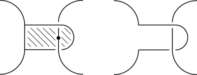
Figure 3. Band-clasping.

In Figure 4 we show a band-clasping of two trefoils. If we can find a projection onto a plane such that the projections of $K$ and $f(D)$ intersect only in the projection of $K\cap f(D)$, then we say that $K^{\prime}\cup J$ is the trivial band-clasping of $K$ and $J$. It is straightforward to see that in that case the resulting link does not depend on the choice of $f$.

$J$ at 185 67 $K$ at 120 83

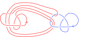
Figure 4. A band-clasping of two trefoils.

We have the following observation about Alexander polynomials of band-claspings.

Proposition 5.1.

Let $L$ be a band-clasping of $K$ and $J$, then

$$\Delta_{L}(s,t)=\Delta_{K}(t)\cdot\Delta_{J}(s)\cdot g\,\overline{g}$$

for some non-zero $g\in\Lambda$. Furthermore $g=1$ if the band-clasping is trivial.

For example, using Kodama’s program knotGTK we can show that for the link $L$ in Figure 4 we have

$$\Delta_{L}(s,t)=(1-s+s^{2})(1-t+t^{2})(s^{-1}-1+t)(s-1+t^{-1}).$$

Note that band-claspings have splitting number $1$. The lemma is thus a consequence of Corollary 4.3, but we prefer to give a sketch of a proof which is particular to this class of links.

Sketched proof of Proposition 5.1.

First of all, it is well-known, and can be shown using a Mayer–Vietoris argument, that the Alexander polynomial of the trivial band-clasping of $K$ and $J$ equals $\Delta_{K}(t)\cdot\Delta_{J}(s)$. Furthermore the proof of [Mi98, Theorem 1.1] carries over to show that any band-clasping $L$ of $K$ and $J$ is in fact ribbon concordant to the trivial band-clasping of $K$ and $J$. (We refer to [Tri69] or alternatively [Sav02, p. 189] for the definition of ribbon concordance.) It then follows from standard arguments, e.g. by a variation on [Ka78, Theorem B], that

$$\Delta_{L}(s,t)=\Delta_{K}(t)\cdot\Delta_{J}(s)\cdot g\,\overline{g}$$

for some non-zero $g\in\Lambda$. ∎

It can be shown by an argument completely analogous to that of [Kon79, Theorem 1], that any 2-component link with splitting number $1$ is a band-clasping of its components. Moreover it seems likely, but we will not provide a proof, that in Proposition 5.1 any non-zero $g$ can be realized by a band-clasping. If this is correct, then this will in particular show, except for determining the negligible factor precisely, that the conclusion of Corollary 4.3 (2) is optimal.

5.3. Splitting numbers

In an earlier paper [CFP13], two of us together with Jae Choon Cha already discussed splitting numbers in detail. In this section we will revisit some of the results from that paper.

First we remind the reader that in the calculation of the splitting number, one only allows crossing changes between different components. It is straightforward to show (see [CFP13, Lemma 2.1]) that the splitting number has the same parity as the sum of all linking numbers $\operatorname{lk}(L_{i},L_{j})$ with $i>j$. For example, if $L$ is a 2-component link with odd linking number, then the splitting number is also necessarily odd.

In [CFP13] Alexander polynomial techniques were used to derive splitting number conclusions for 2-component linking number one links with at least one knotted component. When both components were unknotted, covering link calculus was used, in which one studies the preimage of one component of the link in the covering space branched along the other component; see [CK08, Cha09, CO93] for more on covering link calculus. Some, but not all, of the conclusions obtained in [CFP13] using covering links can be drawn using Corollary 4.3. For example, in [CFP13] we investigated the link $L12n1320$, shown in Figure 5.

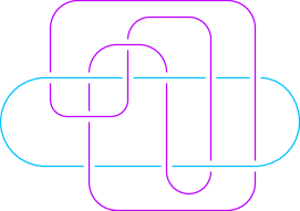
Figure 5. The link $L12n1320$.

This is a 2-component link with linking number one and unknotted components. It was shown in [CFP13, Section 5.2] that the splitting number is 3. According to knotGTK [Kod], the Alexander polynomial is:

$$t_{1}^{3}t_{2}^{3}-2t_{1}^{2}t_{2}^{3}-t_{1}^{3}t_{2}^{2}+t_{1}t_{2}^{3}+5t_{1}^{2}t_{2}^{2}-4t_{1}t_{2}^{2}-4t_{1}^{2}t_{2}+5t_{1}t_{2}+t_{1}^{2}-t_{2}-2t_{1}+1,$$

which factors as

$$(t_{1}-1)(t_{2}-1)(t_{1}^{2}t_{2}^{2}-t_{1}t_{2}^{2}+3t_{1}t_{2}-t_{1}+1).$$

Since the last factor is not a norm, Corollary 4.3 says that the splitting number is greater than 1. In fact by the observation above, the splitting number of $L12n1320$ has to be odd, so it has to be at least 3. In fact it is easy to verify that it is precisely 3. The proof of this fact in [CFP13, Section 5.2] used twisted Alexander polynomials to show that a covering link is not slice, while [BS13] used a Khovanov homology spectral sequence.

Similarly, the links $L8a16$ and $L9a46$ were shown in [CFP13] to have splitting number 3 using covering links. They are 3-component links with nonzero Alexander polynomial, hence we also get from Corollary 4.3 that the splitting number is at least $3$.

Note that for 2- and 3-component links this approach can only show that the splitting number is at least 3, whereas the covering link techniques were sometimes sufficient to show that the splitting number is 5.

5.4. Weak splitting numbers

The 3-component link $L8a16$, shown in Figure 6, has unknotted components and Alexander polynomial

$$(t_{1}-1)(t_{2}-1)(t_{3}-1)(t_{2}t_{3}-1).$$

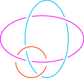
Figure 6. The link $L8a16$.

As well as having unlinking number 3 we see that $L8a16$ also has weak splitting number 3, by Corollary 4.4. Similarly, we can also apply Corollary 4.4 to prove that the link $L12n1320$ considered in Section 5.3 does not have weak splitting number 1.

6. Knot types obtained from weak splitting operations

Recall the following notation from the introduction. If a link $J$ can be obtained from a link $L$ by a sequence of $r$ crossing changes then we write $L\rightsquigarrow_{r}J$. A sequence of crossing changes culminating in a split link is referred to as a splitting sequence. Given knots $K_{1},\dots,K_{m}$ we denote the split link whose components are these knots by $K_{1}\sqcup\dots\sqcup K_{m}$. Also we write $U$ for the unknot.

Given an $m$-component link $L$ with weak splitting number $\operatorname{wsp}(L)=r$, we investigate the question of which knot types can arise in a splitting sequence of length $r$. Theorem 6.1 below concerns the case $r=m-1$.

Theorem 6.1.

Let $L$ be an $m$ component link with $\Delta_{L}\neq 0$ and $\operatorname{wsp}(L)=m-1$. Then for any two splitting sequences $L\rightsquigarrow_{m-1}K_{1}\sqcup\dots\sqcup K_{m}$ and $L\rightsquigarrow_{m-1}J_{1}\sqcup\dots\sqcup J_{m}$ we have

$$\bigoplus_{i=1}^{m}\operatorname{Bl}_{K_{i}}(t_{i})\sim\bigoplus_{i=1}^{m}\operatorname{Bl}_{J_{i}}(t_{i}),$$

where $\sim$ indicates equivalence in the Witt group of linking forms. In particular

$$\prod_{i=1}^{m}\Delta_{K_{i}}(t_{i})\cdot f\,\overline{f}=\prod_{i=1}^{m}\Delta_{J_{i}}(t_{i})\cdot g\,\overline{g}\cdot n$$

for some non-zero polynomials $f,g$ and some negligible $n\in\Lambda$.

Proof.

In this proof write $\mathcal{K}:=K_{1}\sqcup\dots\sqcup K_{m}$ and $\mathcal{J}:=J_{1}\sqcup\dots\sqcup J_{m}$. Since $\Delta_{L}\neq 0$ we have $\beta(L)=0$, while

$$\beta(\mathcal{K})=\beta(\mathcal{J})=r$$

by Lemma 2.4. By Theorem 1.1 we have that $\operatorname{Bl}_{\mathcal{K}}\oplus-\operatorname{Bl}_{L}$ and $\operatorname{Bl}_{\mathcal{J}}\oplus-\operatorname{Bl}_{L}$ are metabolic and therefore both are zero in the Witt group. In particular they are equivalent in the Witt group, from which it follows that $\operatorname{Bl}_{\mathcal{K}}=\operatorname{Bl}_{\mathcal{J}}$ in the Witt group. By Lemma 2.8 the Blanchfield forms of $\mathcal{K}$ and $\mathcal{J}$ are the Witt sums of the Blanchfield forms of their constituent knots.

The second statement is now a consequence of Lemma 2.5 and Lemma 2.6. ∎

Adams [Ad96] gave the first example of a 2-component link $L$ with unknotted components and weak splitting number one, such that any crossing change which splits $L$ necessarily turns one of the two components of $L$ into a nontrivial knot. In the final paragraph of [Ad96] Adams asked (see Question 1.4) whether there exist such examples, where in addition we may guarantee high complexity of a component arising from a single splitting crossing change. The following theorem gives an affirmative answer to Adams’ question.

Theorem 1.5. Fix $c\in\mathbb{N}$. There exists a 2-component link $L$ with unknotted components such that such for any knot $K$ with $L\rightsquigarrow_{1}K\sqcup U$, the crossing number of $K$ is at least $c$.

The proof of Theorem 1.5 will require the remainder of this section. The examples we construct are inspired by the construction of Adams [Ad96], but we remark that we have to change the links from [Ad96] slightly, since the links in [Ad96, Figure 4] are boundary links and therefore have $\Delta_{L}=0$ and $\beta(L)=1$, whereas we require $\Delta_{L}\neq 0$ and $\beta(L)=0$ in order to apply our results.

$T$ at 60 90 $T$ at 360 90

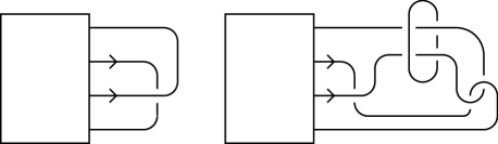
Figure 7. Left: the box denotes a tangle $T$ such that the diagram is an unknotting number one knot with the unknotting crossing isolated. Right: replace the strands outside the box as shown to get a 2-component link $L_{T}$ with unknotted components and weak splitting number one.

Choose $n$ to be such that $2n+1\geq c$. Choose an irreducible Laurent polynomial $\Delta(t)=a_{0}(1+t^{2n})+a_{1}(t+t^{2n-1})+\dots+a_{n-1}(t^{n-1}+t^{n+1})+a_{n}t^{n}$ with $\Delta(1)=1$ and degree $2n$, where $2n=p-1$ for $p$ an odd prime. For example choosing $n$ so that $2n=p-1$ for $p$ an odd prime greater than or equal to $c$, and taking $a_{2i}=1$ and $a_{2i+1}=-1$ for $i=0,\dots,\lfloor n/2\rfloor$ gives rise to such a polynomial, since this is a cyclotomic polynomial and cyclotomic polynomials are irreducible.

According to the main theorem of [Kon79], there exists an unknotting number one knot $J$ with $\Delta_{J}(t)\doteq\Delta(t)$. Let $T$ be a tangle such that the picture on the left hand side of Figure 7 is a diagram for $J$, where we isolated a crossing, at which a crossing change results in an unknot. If necessary, switch $J$ for one of either its reverse $rJ$, its mirror image $\overline{J}$ or $r\overline{J}$, in order to arrange that the orientations are as shown on the left of Figure 7. (These orientations will soon be important for simplifying the construction of a Seifert surface.) Replace the strands outside the box with the arrangement on the right hand side of Figure 7, to obtain a 2-component link with unknotted components which we call $L_{T}$. Changing one crossing of $L_{T}$, in the clasp on the right, yields $J\sqcup U$. This construction is an adaptation of that of [Ad96, Figure 4].

Lemma 6.2.

The links $L_{T}$ constructed above have nonzero Alexander polynomial $\Delta_{L_{T}}\neq 0$.

Before giving the proof we recall the definition of the Sato-Levine invariant of a 2-component link $L=L_{1}\cup L_{2}$ with linking number zero [Sat84]. Pick two Seifert surfaces $F_{1}$ and $F_{2}$ in $S^{3}$, with $\partial F_{i}=L_{i}$, $F_{1}\cap L_{2}=F_{2}\cap L_{1}=\emptyset$ and $F_{1}\pitchfork F_{2}$. The intersection $F_{1}\cap F_{2}$ is a link $J\subset S^{3}$. Choose an orientation of $J$, a framing for the normal bundle of $J$ in $F_{1}$ and a framing for the normal bundle of $J$ in $F_{2}$, such that the first two agree with the orientation of $F_{1}$, the first and the third agree with the orientation of $F_{2}$, and all three agree with the orientation of $S^{3}$. Together the framings of the normal bundles to $J$ in $F_{1}$ and $F_{2}$ give a framing for the normal bundle of $J$ in $S^{3}$. The framed bordism class of the link $J$ then defines the Sato-Levine invariant. Recall that two framed links in $S^{3}$ are framed bordant if and only if the sums of their framing coefficients are equal, since we can use the Pontryagin-Thom construction to produce an element of $\pi_{3}(S^{2})\cong\mathbb{Z}$, with the Hopf invariant yielding the isomorphism to $\mathbb{Z}$.

Proof of Lemma 6.2.

We start with the following claim.

Claim.

The links $L_{T}$ above have Sato-Levine invariant $-1$.

To prove the claim, apply the Seifert algorithm to the left hand component of $L_{T}$, on the right of Figure 7. Call this component $L_{1}$ and the resulting Seifert surface $F_{1}$. Construct a Seifert surface $F_{2}$ for the other component $L_{2}$ by taking the obvious disc and tubing along $L_{1}$ where $L_{1}$ hits the disc, passing the tube around the clasp. This makes Seifert surfaces $F_{1},F_{2}$ for $L_{1},L_{2}$ respectively with $F_{1}\cap L_{2}=\emptyset=F_{2}\cap L_{1}$. The orientation is important for ensuring that the Seifert algorithm gives a surface $F_{1}$ disjoint from $L_{2}$. The intersection $F_{1}\cap F_{2}$ is a single circle and the self linking of $F_{1}\cap F_{2}$ from the framing induced by the Seifert surfaces is $-1$; it can be seen that a full negative twist in the induced framing arises when passing around the clasp. This completes the proof of the claim.

As was shown in [Co85, Theorem 4.1], the Sato-Levine invariant of a 2-component link $L$ with linking number zero is equal to minus the coefficient of $z^{3}$ in the Conway polynomial $\nabla_{L}(z)$. Thus the Conway polynomial is nonzero.

According to Kawauchi [Ka96, Proposition 7.3.14] we may relate the multivariable and single variable Alexander polynomials by:

$$\Delta_{L}(t,t)(t-1)=\Delta_{L}(t).$$

Thus, to show that the multivariable Alexander polynomial is nonzero it suffices to show that $\Delta_{L}(t)\neq 0$. Suppose that $V$ is an $m\times m$ Seifert matrix for $L$ arising from a connected Seifert surface. Then

$$t^{-m/2}\Delta_{L}(t)\doteq\det(t^{1/2}V-t^{-1/2}V^{T})=\nabla_{L}(t^{1/2}-t^{-1/2})=\nabla_{L}(z);$$

the change of variables is $z=t^{1/2}-t^{-1/2}$. Thus if $\Delta_{L}(t)=0$ then $\nabla_{L}(z)=0$. The fact shown above that $\nabla_{L}(z)\neq 0$ therefore completes the proof of Lemma 6.2. ∎

The next result follows immediately from Alexander’s original definition; compare also [Ro76, Exercise 8.C.12, page 208]. The proof is left to the reader. For a Laurent polynomial $p(t)=\sum_{i\in\mathbb{Z}}a_{i}t^{i}\in\mathbb{Z}[t^{\pm 1}]$ we define $\deg(p(t))$ to be the difference $\deg(p(t)):=\max\{j\in\mathbb{Z}\,|\,a_{j}\neq 0\}-\min\{k\in\mathbb{Z}\,|\,a_{k}\neq 0\}$.

Lemma 6.3.

Let $K$ be a nontrivial knot and $c$ be its crossing number. Then the degree of the Alexander polynomial satisfies $\deg\Delta_{K}\leq c-1$.

Continuation of the proof of Theorem 1.5.

Consider the links $L_{T}$ constructed above. We have $L\rightsquigarrow_{1}J\sqcup U$, where $\deg(\Delta_{J})=2n$ and $2n+1\geq c$; recall that $n$ was chosen to satisfy this property with respect to $c$. For any knot $K$ with Alexander polynomial having degree $2n$ we have $2n\leq k-1$, where $k$ is the crossing number of $K$. Thus we have $c\leq 2n+1\leq k$. It therefore suffices to show that any knot $K$ arising from one splitting crossing change on $L_{T}$ has Alexander polynomial containing $\Delta_{J}(t)$ as a factor.

Since $\Delta_{L_{T}}\neq 0$, we have that $\beta(L)=0$, whereas $\beta(J\sqcup U)=1$ by Lemma 2.4. Therefore by Theorem 1.3 and another application of Lemma 2.4 we have that

$$\Delta_{L_{T}}(t_{1},t_{2})=\Delta^{\operatorname{tor}}_{J\sqcup U}\cdot f\,\overline{f}\cdot m=\Delta_{J}(t_{1})\cdot f\,\overline{f}\cdot m$$

for some $f\in\Lambda$ and some negligible $n\in\Lambda$.

Now suppose that we have some other splitting crossing change on $L$ yielding $K\sqcup U$. Then similarly to above we have

$$\Delta_{L_{T}}(t_{1},t_{2})=\Delta^{\operatorname{tor}}_{K\sqcup U}\cdot g\,\overline{g}\cdot m^{\prime}=\Delta_{K}(t_{1})\cdot g\,\overline{g}\cdot m^{\prime}$$

for some $g\in L$ and some negligible $m^{\prime}\in\Lambda$. Therefore

(6.1) $$\Delta_{J}(t_{1})\cdot f\,\overline{f}\cdot m=\Delta_{K}(t_{1})\cdot g\,\overline{g}\cdot m^{\prime}.$$

The ring $\Lambda$ is a UFD and $\Delta_{J}$ is irreducible. Therefore a non–negative number $a_{\Delta_{K}}$ such that $\Delta_{J}^{a_{\Delta_{K}}}$ divides $\Delta_{K}$, but $\Delta_{J}^{1+a_{\Delta_{K}}}$ does not, is well–defined. Similarly we define $a_{f}$, $a_{\overline{f}}$, $a_{g}$, $a_{\overline{g}}$. As $\Delta_{J}$ is symmetric, we infer that $a_{f}=a_{\overline{f}}$ and $a_{g}=a_{\overline{g}}$. Notice that $\Delta_{J}$, being a non–trivial knot polynomial, does not divide negligible polynomials $m$ and $m^{\prime}$.

The maximal exponent $a$ such that $\Delta_{J}$ divides the left hand side of (6.1) is $1+2a_{f}$. For the right hand side it is $a_{\Delta_{K}}+2a_{g}$. This implies that $a_{\Delta_{K}}$ is odd, in particular $\Delta_{J}$ divides $\Delta_{K}$. This shows that $\deg\Delta_{K}\geq\deg\Delta_{J}=2n$. Recall that $n$ was chosen so that $2n+1\geq c$, and by Lemma 6.3 this implies that the crossing number of $K$ is at least $c$. ∎

7. Questions

Kohn [Koh93] initiated the study of unlinking numbers for links with more than one component. There are five 2-component 9 crossing links for which Kohn could not compute the unlinking number, namely

$$9^{2}_{3}=L9a30,9^{2}_{15}=L9a15,9^{2}_{27}=L9a17,9^{2}_{31}=L9a2\mbox{ and }9^{2}_{36}=L9a10,$$

where the names come from Rolfsen’s book [Ro76] and the Linkinfo tables [CL] respectively. For each link the question is whether the unlinking number is two or three. Kanenobu recently announced a proof that the unlinking number of $L9a30$ is 3. Unfortunately the techniques of this paper do not help. It would be very interesting if it could be shown that one of the four remaining links has unlinking number 3.

References

- [Ad96] C. Adams, Splitting versus unlinking, J. Knot Theory Ramifications 5 (1996), 295–299.
- [BS13] J. Batson and C. Seed, A Link Splitting Spectral Sequence in Khovanov Homology, preprint (2013).
- [Bl57] R. C. Blanchfield, Intersection theory of manifolds with operators with applications to knot theory, Ann. of Math. 65 (1957), 340–356.
- [BW84] M. Boileau and C. Weber. Le problème de J. Milnor sur le nombre gordien des nœuds algébriques Enseign. Math. 30 (1984), 173-222.
- [BF12] M. Borodzik and S. Friedl, The unknotting number and classical invariants I, preprint (2012), to be published by Alg. Geom. Top.
- [BF13] M. Borodzik and S. Friedl, On the algebraic unknotting number, preprint (2013), arXiv:1308.6105. To be published by the Trans. Lond. Math. Soc.
- [Cha09] J. C. Cha, Structure of the string link concordance group and Hirzebruch-type invariants, Indiana Univ. Math. J. 58 (2009), no.2, 891–927.
- [CK08] J. C. Cha and T. Kim, Covering link calculus and iterated Bing doubles, Geometry and Topology 12 (2008), 2173–2201.
- [CFP13] J. C. Cha, S. Friedl and M. Powell, Splitting numbers of links, preprint (2013), arXiv:1308.5638.
- [CP14] J. C. Cha, M. Powell, Covering link calculus and the bipolar filtration of topologically slice links. Geom. Topol. 18 (2014), no. 3, 1539–1579.
- [Ch74] T. A. Chapman, Topological invariance of Whitehead torsion, Amer. J. Math. 96 (1974), 488–497.
- [CL] J. C. Cha and C. Livingston, LinkInfo: Table of link invariants, http://www.indiana.edu/~linkinfo/.
- [Co85] T. D. Cochran, Concordance invariance of coefficients of Conway’s link polynomial, Invent. Math. 82 (1985), no. 3, 527–541.
- [CO93] T. D. Cochran and K.E. Orr, Not all links are concordant to boundary links, Ann. of Math. (2) 138 (1993), no. 3, 519–554.
- [COT03] T. D. Cochran, K. E. Orr and P. Teichner, Knot concordance, Whitney towers and -signatures, Annals of Mathematics 157 (2003), 433–519.
- [CF77] R. H. Crowell and R .H. Fox, Introduction to Knot Theory, Second revised edition, Graduate Texts in Mathematics 57, Springer-Verlag, Berlin - Heidelberg - New York (1977).
- [FHH89] T. H. Fay, K. A. Hardie and P. J. Hilton, The two-square lemma, Publicacions Matemàtiques 33 (1989) No. 1, 133–137.
- [FP12] S. Friedl and M. Powell, Cobordisms to weakly splittable links, Proc. Amer. Math. Soc. 142 (2014), 703-712.
- [GS99] R. Gompf, A. Stipsicz, -manifolds and Kirby calculus, Graduate Studies in Mathematics, 20. American Mathematical Society, Providence, RI, 1999
- [Hi12] J. Hillman, Algebraic invariants of links, second edition, Series on Knots and Everything, 52. World Scientific Publishing Co. Inc, River Edge, NJ, (2012).
- [HS71] P. Hilton and U. Stammbach, A Course in Homological Algebra, Grad. Texts in Math. 4, Springer Verlag, New York (1971).
- [Ka78] A. Kawauchi, On the Alexander polynomials of cobordant links, Osaka J. Math. 15 (1978), 151–159.
- [Ka96] A. Kawauchi, Distance between links by zero-linking twists, Kobe J. Math. 13 (1996), No. 2, 183–190.
- [Ka13] A. Kawauchi, The Alexander polynomials of immersed concordant links, preprint (2013), to appear in Boletin de la Sociedad Matematica Mexicana.
- [Kim14] M. H. Kim, Whitney towers, Gropes and Casson-Gordon style invariants of links, preprint (2013) arXiv:1405.5722.
- [Kir89] R. C. Kirby, The topology of -manifolds, Lecture Notes in Mathematics 1374, Springer-Verlag, Berlin (1989).
- [Kod] K. Kodama, KnotGTK, http://www.math.kobe-u.ac.jp/~kodama/knot.html
- [Koh91] P. Kohn, Two-bridge links with unlinking number one, Proc. Amer. Math. Soc. 113 (1991), No. 4, 1135–1147.
- [Koh93] P. Kohn, Unlinking two component links, Osaka J. Math. 30 (1993), No. 4, 741–752.
- [Kon79] H. Kondo, Knots of unknotting number and their Alexander polynomials, Osaka J. Math. 16 (1979), No. 2, 551–559.
- [La14] M. Lackenby, Elementary knot theory, to be published by the Clay Mathematics Institute (2014)
- [Let00] C. F. Letsche, An obstruction to slicing knots using the eta invariant, Math. Proc. Camb. Philos. Soc. 128 (2000), 301–319.
- [Mi98] K. Miyazaki, Band-sums are ribbon concordant to the connected sum, Proc. Am. Math. Soc. 126 (1998), 3401–3406.
- [Ne81] W. Neumann, A calculus for plumbing applied to the topology of complex surface singularities and degenerating complex curves, Trans. Am. Math. Soc. 268(1981), 299–343.
- [Ni03] L. I. Nicolaescu The Reidemeister torsion of 3-manifolds, de Gruyter Studies in Mathematics 30, Walter de Gruyter & Co. Berlin, (2003).
- [Sh12] A. Shimizu, The complete splitting number of a lassoed link, Topology Appl. 159 (2012), 959–965.
- [Ro76] D. Rolfsen, Knots and links, Mathematics Lecture Series, No. 7, Publish or Perish Inc, Berkeley, Calif. (1976).
- [Sat84] N. Sato, Cobordisms of semiboundary links, Topology Appl. 18 (1984), No. 2-3, 225–234.
- [Sav02] N. Saveliev, Invariants for homology 3-spheres, Encyclopaedia of Mathematical Sciences. Low-Dimensional Topology. 140 (2012)
- [Tra88] L. Traldi, Conway’s potential function and its Taylor series, Kobe Journal of Mathematics 5 (1988), 233–264.
- [Tri69] A. G. Tristram, Some cobordism invariants for links, Proc. Camb. Philos. Soc. 66 (1969), 251–264.
- [Tu01] V. Turaev, An introduction to combinatorial torsion, Notes taken by Felix Schlenk, Lectures in Mathematics ETH Zürich, Birkhäuser Verlag, Basel (2001).