Non-linear collisionless damping of Weibel turbulence in relativistic blast waves

Abstract

The Weibel/filamentation instability is known to play a key role in the physics of weakly magnetized collisionless shock waves. From the point of view of high energy astrophysics, this instability also plays a crucial role because its development in the shock precursor populates the downstream with a small-scale magneto-static turbulence which shapes the acceleration and radiative processes of suprathermal particles. The present work discusses the physics of the dissipation of this Weibel-generated turbulence downstream of relativistic collisionless shock waves. It calculates explicitly the first-order non-linear terms associated to the diffusive nature of the particle trajectories. These corrections are found to systematically increase the damping rate, assuming that the scattering length remains larger than the coherence length of the magnetic fluctuations. The relevance of such corrections is discussed in a broader astrophysical perspective, in particular regarding the physics of the external relativistic shock wave of a gamma-ray burst.

52.27.Ny, 52.25.Fi

1 Introduction

The physics of collisionless shock waves has drawn wide interest, from pure theoretical plasma physics, starting with the pioneering work of Moiseev & Sagdeev (1963), to high energy astrophysics (e.g. Blandford & Eichler, 1987), where it plays a key role in explaining most of the observed non-thermal spectra, and more recently, to laboratory high energy density physics, where collisionless shock waves are about to be produced through the interactions of laser beam-generated plasmas (e.g. Drake & Gregori, 2012). At low magnetization – meaning that the unshocked plasma carries a magnetic field of small energy density compared to the shock kinetic energy – the physics of these collisionless shock waves is driven by the filamentation instability, also dubbed Weibel instability: this filamentation instability takes place in the shock precursor, where the incoming background plasma – as viewed in the reference frame in which the shock lies at rest – mixes with a population of shock-reflected or supra-thermal particles. This has been demonstrated by ab initio Particle-in-Cell (PIC) simulations, see e.g. Kato & Takabe (2008) for non-relativistic unmagnetized shock waves and Spitkovsky (2008a) for their relativistic counterparts, of direct interest to the present work. This filamentation instability and its various branches have consequently received a great deal of attention (see e.g. for relativistic shock waves Medvedev & Loeb, 1999; Wiersma & Achterberg, 2004; Lyubarsky & Eichler, 2006; Achterberg & Wiersma, 2007; Achterberg et al., 2007; Bret et al., 2010; Lemoine & Pelletier, 2010; Rabinak et al., 2011; Lemoine & Pelletier, 2011; Shaisultanov et al., 2012).

Further simulations by Spitkovsky (2008b) have shown that, not only can Weibel / filamentation build up the electromagnetic barrier which gives rise to the shock transition through the isotropisation of the incoming background plasma, it also builds up the turbulence which is transmitted downstream of the shock, on plasma skin depth scales, and which provides the scattering centers for the Fermi acceleration process. Actually, the excitation of micro-turbulence – meaning a turbulence on scales smaller than the typical gyro-radius of accelerated particles – is a necessary condition for a proper relativistic Fermi process (Lemoine et al., 2006; Niemiec et al., 2006).

Additionally, Medvedev & Loeb (1999) have suggested that the filamentation mode is able to build up the turbulence in which the accelerated particles can lose their energy to secondary radiation through synchrotron (and possibly synchrotron self-Compton) processes. In this unified picture, the filamentation instability that develops in the shock precursor would explain a variety of phenomena, from shock formation, to shock acceleration and even the non-thermal radiation from powerful astrophysical sources such as gamma-ray bursts. More particularly, the so-called gamma-ray burst afterglow radiation is attributed to the acceleration and (synchrotron) radiation of electrons at the external shock of the gamma-ray burst ultra-relativistic outflow, as it impinges on the very weakly magnetized circumburst medium. The phenomenological model of the afterglow provides a satisfactory description of most observed multi-wavelength afterglow light curves, see e.g Piran (2004).

A notorious problem of the afterglow model remains to explain the origin of the magnetic field that permeates the blast, in which the electrons are assumed to radiate. Indeed, the turbulence which is generated through the Weibel/filamentation instability in the shock precursor and transmitted downstream is expected to decay rather quickly, on multiples of the skin depth scale (Gruzinov & Waxman, 1999), while the time scales on which the electrons cool through synchrotron is of the order of $10^{8}\,\omega_{\rm p}^{-1}$ for typical external conditions. This remark has spurred many theoretical and numerical studies on energy transfer processes to long wavelengths (e.g. Medvedev et al., 2005; Katz et al., 2007), or alternative instabilities, which might re-amplify the magnetic field to a fraction of equipartition, from e.g. the interaction of the shock with an inhomogeneous medium (Sironi & Goodman, 2007; Mizuno et al., 2014), or from a Rayleigh-Taylor instability at the contact discontinuity (Gruzinov, 2000; Levinson, 2009, 2010). How fast the Weibel-generated turbulence decays thus appears to be a key ingredient in shaping the light curves of relativistic blast waves.

Recent PIC simulations have addressed this dissipation issue. In PIC simulations of a relativistic collisionless pair shock up to time $5300\,\omega_{\rm p}^{-1}$, Chang et al. (2008) have observed an isotropic, magneto-static turbulence downstream of the shock, which decays through phase mixing with a damping rate in rough agreement with the theoretical linear estimate. However, these authors point out that the linear calculation is ill-suited to describe the damping of the Weibel-generated turbulence in relativistic blast waves, since the trajectories of particles deviate from the ballistic regime. This remark has motivated the present study, which proposes to evaluate the first non-linear corrections to the damping rate of such Weibel-generated turbulence, accounting for the deviation of particle trajectories from straight lines.

The PIC simulations of Chang et al. (2008) have been essentially confirmed by the more extensive simulations of Keshet et al. (2009), although the latter authors observe that the acceleration of particles to progressively higher energies back reacts on the structure of the shock, and more importantly, on the power spectrum of the downstream turbulence, as suggested independently by Medvedev & Zakutnyaya (2009). Therefore, the former study concludes that present PIC simulations have not yet converged to a steady state. Since this longest PIC simulation ($\sim 10^{4}\,\omega_{\rm p}^{-1}$) represents only a fraction of a percent of the dynamical timescale of the external shock wave of an actual gamma-ray burst, while particle acceleration and cooling is believed to take place on up to this latter timescale, this also means that theoretical extrapolation is needed to bridge the gap between these simulations and actual objects. Therefore, the damping rate, which depends on the power spectrum of the magnetic field, may well differ from that measured in these PIC simulations. This will be discussed in some detail further on.

In order to evaluate the non-linear corrections to Landau damping, the present work calculates the non-linear susceptibility in a magneto-static turbulence, following the Dupree-Weinstock description of resonance broadening (Dupree, 1966; Weinstock, 1969, 1970; Ben-Israel et al., 1975). This picture has been used in many studies to evaluate the saturation of instabilities through the back-reaction of particle diffusion in the grown turbulence, see e.g. Dum & Dupree (1970), Bezzerides & Weinstock (1972), Weinstock (1972), Weinstock & Bezzerides (1973) and later works, e.g. Pokhotelov & Amariutei (2011) for the particular case of the Weibel temperature anisotropy. Here, it is used in a different context: downstream of the shock, the turbulence is magneto-static and isotropic, therefore the plasma is not subject to any instability, only to dissipation through phase mixing; the Dupree-Weinstock approach nevertheless allows to account for the influence of non-ballistic trajectories on the damping rate. Actually, it will be shown that a complete calculation of the first order non-linear corrections is possible, since one can calculate explicitly the trajectory correlators in a magneto-static small-scale turbulence, following the method developed in Pelletier (1977) and Plotnikov et al. (2011).

The results obtained indicate a correction of order unity at the first non-linear order. However, they also indicate that the correction systematically increases the damping rate, and that the magnitude of the correction vs the maximal wavenumber of the turbulence depends on the power spectrum of the magnetic field. These results are discussed in a broad context in Sec. 4. Section 2 provides the background for the calculation of the non-linear damping rate, which is explicitly evaluated in Sec. 3. The trajectory correlators, which enter the calculation, are discussed in a separate Appendix B.

2 Non-linear damping of small-scale magnetostatic turbulence

The initial set-up can be described as follows, in the rest frame of the (downstream) shocked plasma. Time $t=0$ corresponds to the time at which a given plasma element is advected through the shock towards downstream; while this plasma element has been crossing the shock precursor, it has been exposed to micro-instabilities which have built up a microturbulence to a level characterized by the parameter $\epsilon_{B}$:

$$\epsilon_{B}\,=\,\frac{\left\langle\delta B^{2}\right\rangle}{4\pi\left(\gamma_{\rm rel}-1\right)nmc^{2}}$$ (1)

with $m=m_{\rm i}$ for an electron-ion shock, $m=m_{e}$ for a pair shock; $n$ represents the particle density in the downstream plasma rest frame, and $\gamma_{\rm rel}$ represents the Lorentz factor of the upstream plasma in the downstream rest frame; if $\gamma_{\rm sh}\,\equiv\,\left(1-\beta_{\rm sh}^{2}\right)^{-1/2}$ denotes the Lorentz factor of the shock front (and $\beta_{\rm sh}$ its velocity in units of $c$) relatively to the upstream plasma, $\gamma_{\rm rel}\,\simeq\,\gamma_{\rm sh}/\sqrt{2}$ for a strong relativistic weakly magnetized shock (Blandford & McKee, 1976). PIC simulations yield a value $\epsilon_{B}\,\sim\,10^{-3}-10^{-2}$ immediately downstream of the shock (Keshet et al., 2009). The following calculations describe the microturbulence as aperiodic, i.e. $\Re\omega\,=\,0$, homogeneous and isotropic, as indicated by PIC simulations, see in particular Chang et al. (2008).

In this respect, the present set-up differs from that of Mart’yanov et al. (2008) and Kocharovsky et al. (2010) which derive stationary non-linear and coherent magneto-static solutions to the Vlasov-Maxwell system in terms of inhomogeneous and anisotropic particle distribution functions. Such structures indeed emerge in the shock precursor in the non-linear phase of the instability, as a balance between the anisotropy/inhomogeneity of the particle distribution functions and the magnetic forces. In the present case, the downstream particle distribution function is assumed homogeneous and isotropic, therefore the plasma is prone to collisionless damping. The homogeneity and isotropicity of the distribution function in the downstream plasma is a direct consequence of the shock transition, as clearly revealed by PIC simulations.

The present microturbulence also differs from the spontaneous turbulence associated to the thermal fluctuations of the plasma, as studied recently by  Felten et al. (2013), Felten & Schlickeiser (2013a), Felten & Schlickeiser (2013b), Ruyer et al. (2013) or Yoon et al. (2014), since the present turbulence has been sourced in the shock precursor by the anisotropies of particle distribution functions.

Finally, the present work neglects any background magnetic field; in the case of the external shock wave of a gamma-ray burst, this is a very good approximation, since the magnetization parameter $\sigma\,\equiv\,B_{\rm ISM|d}^{2}/\left[4\pi\left(\gamma_{\rm rel}-1\right)nmc^{2}\right]$ expressed in terms of the downstream frame background field $B_{\rm ISM|d}$ is very small compared to $\epsilon_{B}$: $\sigma\,\sim\,10^{-9}$ for typical interstellar conditions. Furthermore, the development of the relativistic Fermi acceleration process requires $\sigma\,\ll\,\epsilon_{B}^{2}$ (Pelletier et al., 2009; Lemoine & Pelletier, 2010), i.e. a weakly magnetized shock wave in which the effects of the background magnetic field can be neglected.

2.1 Damping of magneto-static turbulence

Following Chang et al. (2008), one can use Poynting’s theorem to derive the damping rate as a function of the transverse susceptibility. For random electric $\boldsymbol{\delta E}$ and magnetic fields $\boldsymbol{\delta B}$ and random current density fluctuations $\boldsymbol{\delta j}$ with zero spatial average, Maxwell equations imply

$$\frac{1}{8\pi c}\frac{\partial\delta B^{2}}{\partial t}+\frac{1}{8\pi c}\frac{\partial\delta E^{2}}{\partial t}+\frac{1}{c}\boldsymbol{\delta j}\cdot\boldsymbol{\delta E}+\boldsymbol{\nabla}\cdot\left(\boldsymbol{\delta E}\times\boldsymbol{\delta B}\right)\,=\,0\ .$$ (2)

Then, taking the average over space, assuming homogeneous turbulence of strongly magnetic nature, which implies $\boldsymbol{\nabla}\cdot\left\langle\boldsymbol{\delta E}\times\boldsymbol{\delta B}\right\rangle\,=\,0$ and $\delta E^{2}\,\ll\,\delta B^{2}$, one arrives at

$$\frac{1}{8\pi}\frac{{\rm d}\left\langle\delta B^{2}\right\rangle}{{\rm d}t}\,=\,-\left\langle\boldsymbol{\delta j}\cdot\boldsymbol{\delta E}\right\rangle\ ,$$ (3)

or

$$\frac{1}{8\pi}\frac{{\rm d}\left\langle\delta B^{2}\right\rangle}{{\rm d}t} \,=\, -\frac{1}{2}\int\frac{{\rm d}^{3}k}{(2\pi)^{3}}\frac{{\rm d}\omega}{2\pi}\,\frac{{\rm d}^{3}k^{\prime}}{(2\pi)^{3}}\frac{{\rm d}\omega^{\prime}}{2\pi}\left\langle\boldsymbol{\delta j_{k\omega}}\cdot\boldsymbol{\delta E_{k^{\prime}\omega^{\prime}}^{\star}}+\boldsymbol{\delta j_{k\omega}^{\star}}\cdot\boldsymbol{\delta E_{k^{\prime}\omega^{\prime}}}\right\rangle$$ (4)

$$\,=\, \int\frac{{\rm d}^{3}k}{(2\pi)^{3}}\frac{{\rm d}\omega}{2\pi}\,\Im\left(\frac{1}{\omega\chi_{k\omega,\rm T}}\right){\cal S}_{\delta j}(k,\omega).$$

The last equality uses the relation $\boldsymbol{\delta E_{k\omega}}\,=\,i\,\boldsymbol{\delta j_{k\omega}}/\left(\omega\chi_{k\omega,\rm T}\right)$, $\chi_{k\omega,\rm T}$ denoting the transverse susceptibility in $\omega-k$ space. It also introduces the power spectrum of current density fluctuations, through $\langle\delta j_{k\omega}\delta j_{k^{\prime}\omega^{\prime}}^{\star}\rangle\,=\,(2\pi)^{4}\delta\left(\boldsymbol{k}-\boldsymbol{k^{\prime}}\right)\delta(\omega-\omega^{\prime}){\cal S}_{\delta j}(k,\omega)$.

The transverse current density fluctuations are related to the transverse magnetic modes through (Felten et al., 2013)

$$\boldsymbol{\delta j_{k\omega}}\,=\,\frac{i}{4\pi}\boldsymbol{k}c\times\boldsymbol{\delta B_{k\omega}}\left[1+\frac{|\omega|^{4}}{(kc)^{4}}\right]\ .$$ (5)

One can safely neglect the last term in the brackets since $|\omega|=\gamma_{k}$, the damping rate, and $\gamma_{k}\,\ll\,kc$ as demonstrated further on. Therefore the power spectra of current fluctuations and magnetic turbulence are related through ${\cal S}_{\delta j}(k,\omega)\,=\,(kc/4\pi)^{2}{\cal S}_{\delta B}(k,\omega)$ and for magneto-static turbulence, ${\cal S}_{\delta B}(k,\omega)\,=\,2\pi\delta(\omega)\,{\cal S}_{\delta B}(k)$. One thus finally arrives at

$$\frac{{\rm d}\left\langle\delta B^{2}\right\rangle}{{\rm d}t}\,=\,-2\int\frac{{\rm d}^{3}k}{(2\pi)^{3}}\,\gamma_{k}\,{\cal S}_{\delta B}(k)\ ,$$ (6)

with damping rate in $k-$space ($\gamma_{k}$ is counted as positive for effective damping):

$$\gamma_{k}\,=\,-k^{2}c^{2}\Im\left(\frac{1}{4\pi\omega\chi_{k\omega,\rm T}}\right)_{\omega\rightarrow 0}\ .$$ (7)

Therefore, the bulk of the calculation consists in evaluating the non-linear susceptibility. For reference, assuming ballistic trajectories and low frequencies $\omega\,\ll\,kc$, one has

$$4\pi\chi_{k\omega,\rm T}\,\simeq\,-i\frac{\pi}{4}\sum_{\alpha}\frac{4\pi q_{\alpha}^{2}}{\omega k}\,\int{\rm d}p\,p^{2}\frac{{\rm d}\overline{f}_{\alpha}}{{\rm d}p}\,\Theta\left[1-\left(\frac{\omega}{kv}\right)^{2}\right]\,+\,{\cal O}(\omega^{0})\ ,$$ (8)

where $\overline{f}_{\alpha}(p)$ represents the homogeneous part of the distribution function of particles of species $\alpha$. For a Jüttner-Synge distribution:

$$\overline{f}_{\alpha}(p)\,=\,\frac{n_{\alpha}\mu}{4\pi m^{3}c^{3}K_{2}(\mu)}e^{-\mu\gamma}\,$$ (9)

with $\mu=mc^{2}/(kT)$, $\gamma=\left[1+p^{2}/(mc)^{2}\right]^{1/2}$ and $n_{\alpha}$ the density of particles, one finds as $\omega\,\rightarrow\,0$

$$4\pi\chi_{k\omega,\rm T}\,\simeq\,i\frac{\pi}{4}\sum_{\alpha}\frac{\omega_{\rm p,\alpha}^{2}}{\omega kc}\frac{1}{K_{2}(\mu)}\left(\frac{2}{\mu}+\frac{2}{\mu^{2}}\right)e^{-\mu}\ ,$$ (10)

in terms of the relativistic plasma frequency (squared) $\omega_{\rm p,\alpha}^{2}\,=\,4\pi n_{\alpha}q_{\alpha}^{2}\mu/m$ which leads to the ultra-relativistic ($\mu\,\rightarrow\,0$) linear damping rate

$$\gamma_{k}\,\simeq\,\frac{4}{\pi}\frac{k^{3}c^{3}}{\omega_{\rm p}^{2}}\ ,$$ (11)

with $\omega_{\rm p}^{2}\,=\,\sum_{\alpha}\omega_{\rm p,\alpha}^{2}$ the relativistic plasma frequency of the global plasma. This result for the linear Landau damping rate in a ultra-relativistic plasma matches previous derivations, e.g. Bergman & Eliasson (2001), Chang et al. (2008) and Felten & Schlickeiser (2013b).

One can generalize very easily the above result to a power-law distribution of particles with index $s$ and minimum Lorentz factor $\gamma_{\rm min}$:

$$\overline{f}_{\alpha}(p)\,=\,\frac{n_{\alpha}\,|s-1|}{4\pi m^{3}c^{3}\gamma_{\rm min}}\left(\frac{\gamma}{\gamma_{\rm min}}\right)^{-s-2}\,\Theta(\gamma-\gamma_{\rm min})\ .$$ (12)

One then infers in the ultra-relativistic limit $\gamma_{\rm min}\,\gg\,1$

$$\gamma_{k}\,=\,\frac{4}{\pi}\frac{k^{3}c^{3}}{\omega_{\rm p}^{2}}\frac{s}{|(s+2)(s-1)|}\ .$$ (13)

The damping rate differs from the previous by a factor of order unity only. In the following, the calculation of the non-linear damping rate will be carried out for this power-law distribution function, since it guarantees that there are no particle with Lorentz factor outside the range of application of the approximation used (see further below). Furthermore, one expects the distribution function in astrophysical blast waves to follow such a power-law to a good approximation; notably, Fermi acceleration at relativistic shock waves predicts a spectral index $s\,\simeq\,2.3$ in the ultra-relativistic limit for isotropic scattering (e.g. Bednarz & Ostrowski, 1998; Kirk et al., 2000; Achterberg et al., 2001; Lemoine & Pelletier, 2003; Keshet & Waxman, 2005).

2.2 Non-linear susceptibility

The current density fluctuations, from which one can extract the susceptibility, are defined in terms of the fluctuating part of the distribution function, as:

$$\boldsymbol{\delta j}\,=\,\sum_{\alpha}q_{\alpha}\int{\rm d}^{3}r\,\,\boldsymbol{v}\,\delta f_{\alpha}(\boldsymbol{r},\boldsymbol{p},t)\ .$$ (14)

The full distribution function is written $f_{\alpha}(\boldsymbol{r},\boldsymbol{p},t)\,=\,\overline{f}_{\alpha}(\boldsymbol{p},t)+\delta f_{\alpha}(\boldsymbol{r},\boldsymbol{p},t)$, with $\delta f_{\alpha}(\boldsymbol{r},\boldsymbol{p},t)$ the random inhomogenous part and $\overline{f}_{\alpha}(\boldsymbol{p},t)$ the spatial average. Following Weinstock (1969), Weinstock (1970), Ben-Israel et al. (1975) this fluctuating part is given by the solution to the inhomogeneous part of the Boltzmann equation, and it can be written in terms of a propagator ${\cal U_{A}}$ as:

$$\delta f_{\alpha}(\boldsymbol{r},\boldsymbol{p},t)\,=\,{\cal U_{A}}(t,t_{0})\delta f_{\alpha}(\boldsymbol{r},\boldsymbol{p},t_{0})-\int_{t_{0}}^{t}{\rm d}\tau\,\,{\cal U_{A}}(t,\tau)\,\boldsymbol{\delta{\cal F}}(\tau)\cdot\frac{{\rm d}\overline{f}_{\alpha}(\boldsymbol{p},\tau)}{{\rm d}\boldsymbol{p}}\ .$$ (15)

The random force operator is $\boldsymbol{\delta{\cal F}}(\tau)\,\equiv\,q_{\alpha}\left[\boldsymbol{\delta E}(\boldsymbol{r},\tau)+\boldsymbol{v}\times\boldsymbol{\delta B}(\boldsymbol{r},\tau)/c\right]$. In the following, $\overline{f}_{\alpha}$ is assumed isotropic in $p$; then the term associated to the magnetic Lorentz force vanishes in the above expression.

The properties of ${\cal U_{A}}$ are described in details in the above references and its relation to other propagators is discussed in Birmingham & Bornatici (1971). For the sake of completeness, their definitions are recalled in Appendix A.

In the following, the initial data will be written ${\rm init.\,data}$ out of brevity and clarity. Going over to Fourier variables,

$$\delta f_{\alpha\,\boldsymbol{k}}(\boldsymbol{p},t) \,=\, {\rm init.\,data}-$$

$$q_{\alpha}\,\int{\rm d}^{3}r\int\frac{{\rm d}^{3}k^{\prime}}{(2\pi)^{3}}\,e^{-i\boldsymbol{k}\cdot\boldsymbol{r}}\int_{t_{0}}^{t}{\rm d}\tau\,\,{\cal U_{A}}(t,\tau)\,e^{i\boldsymbol{k^{\prime}}\cdot\boldsymbol{r}}\boldsymbol{\delta E_{k^{\prime}}}(\tau)\cdot\frac{\boldsymbol{v}}{v}\frac{{\rm d}}{{\rm d}p}\overline{f}_{\alpha}(p,t)\ .$$

So far, the treatment has been exact; in particular, the separation of $f_{\alpha}(\boldsymbol{r},\boldsymbol{p},t)$ into an average and a random part does not imply any linearisation procedure. The main approximation of the present work is to approximate the full propagator ${\cal U_{A}}$ by the average propagator $\overline{\cal U}$, which corresponds to the truncation to the first term in a series expansion in powers of the fields, see App. A, which summarizes the properties of these propagators, and see most notably Dupree (1966), Weinstock (1969), Weinstock (1970), Birmingham & Bornatici (1971) and Ben-Israel et al. (1975). As recalled in App. A, higher order terms are suppressed relative to this first order correction by powers of $c\tau_{\rm c}/r_{\rm g}$, with $\tau_{\rm c}$ the correlation time of the electromagnetic fluctuations, $r_{\rm g}$ the typical gyroradius of the particles in the turbulence, defined with respect to $\langle\delta B^{2}\rangle^{1/2}$. The present work thus makes the explicit assumption that $r_{\rm g}\,>\,c\tau_{\rm c}$.

In relativistic blast waves, the typical Lorentz factor of a particle downstream of a relativistic shock wave of Lorentz factor $\gamma_{\rm sh}$ is $\gamma_{\rm sh}$ for a pair shock, or $\gamma_{\rm sh}$ (resp. $\gamma_{\rm sh}m_{\rm i}/m_{e}$) for the ion (resp. electron) population in an electron-ion shock (e.g. Spitkovsky, 2008a, b). In the following, this Lorentz factor is denoted $\gamma_{\rm min}$. One then derives the typical ratio $r_{\rm g}/c\tau_{\rm c}$ for a particle of Lorentz factor $\gamma$:

$$\frac{r_{\rm g}}{c\tau_{\rm c}}\,\simeq\,\epsilon_{B}^{-1/2}\frac{k_{\rm max}c}{\omega_{\rm p}}\frac{\gamma}{\gamma_{\rm min}}\ ,$$ (17)

The typical scale of Weibel turbulence is $c\tau_{\rm c}\,=\,k_{\rm max}^{-1}\,\sim\,{\cal K}\,c/\omega_{\rm p}$ with ${\cal K}\,\simeq\,10$ close to the shock front (Spitkovsky, 2008a; Chang et al., 2008; Keshet et al., 2009; Sironi et al., 2013). Given that $\epsilon_{B}\,\lesssim\,10^{-2}$, this indicates that typically, $r_{\rm g}\,\gtrsim\,c\tau_{\rm c}$, possibly $r_{\rm g}\,\gg\,c\tau_{\rm c}$, depending on $\gamma/\gamma_{\rm min}$ and $\epsilon_{B}$. The expansion used here should therefore be a good approximation away from the shock front, where $\epsilon_{B}\,\lesssim\,10^{-2}$.

It is instructive to rewrite the above expansion parameter in terms of the ratio of fluctuating to mean quantities. In particular, using Eq. (5), which relates the current fluctuations to the magnetic fluctuations, one can show that, in orders of magnitude, $\delta n/n\,\sim\,k_{\rm max}c\,\delta B_{k_{\rm max}}/(nec)\,\sim\,\epsilon_{B}^{1/2}k_{\rm max}c/\omega_{\rm p}$, with $\delta n$ the density of current-carrying fluctuations. Therefore the above hierarchy $r_{\rm g}/(c\tau_{\rm c})\,>\,1$ at $\gamma_{\rm min}$ also implies $\delta n\,<\,n$, i.e. small fluctuations; note that the former constraint $r_{\rm g}/(c\tau_{\rm c})\,>\,1$ is more stringent than the latter $\delta n\,<\,n$, because ${\cal K}\,\gtrsim\,10$.

Since $\boldsymbol{\delta E_{k^{\prime}}(\tau)}$ depends solely on time, it commutes with ${\cal U_{A}}$ (see App. A). Equation (LABEL:eq:fakbolt) can then be approximated as

$$\delta f_{\alpha\,\boldsymbol{k}}(\boldsymbol{p},t)\,=\,{\rm init.\,data}-$$

$$\quad\quad q_{\alpha}\,\int{\rm d}^{3}r\int\frac{{\rm d}^{3}k^{\prime}}{(2\pi)^{3}}\,e^{-i\boldsymbol{k}\cdot\boldsymbol{r}+i\boldsymbol{k^{\prime}}\cdot\boldsymbol{r}}\int_{t_{0}}^{t}{\rm d}\tau\,\boldsymbol{\delta E_{k^{\prime}}(\tau)}\cdot\left\langle\,e^{i\boldsymbol{k^{\prime}}\cdot\boldsymbol{\Delta r_{s}}(\tau)}\frac{\boldsymbol{v_{s}}(\tau)}{v_{s}}\frac{{\rm d}\overline{f}_{\alpha}(p,\tau)}{{\rm d}p}\right\rangle\ .$$

The quantities $\boldsymbol{r_{s}}(\tau)$ and $\boldsymbol{v_{s}}(\tau)$ represent the exact orbits of the particles in the fluctuating fields at time $\tau$ with boundary conditions $\boldsymbol{r_{s}}(t)=\boldsymbol{r}$, $\boldsymbol{v_{s}}(t)=\boldsymbol{v}$; furthermore, $\boldsymbol{\Delta r_{s}}(\tau)=\boldsymbol{r_{s}}(\tau)-\boldsymbol{r}$. The average over the exact orbits will be calculated further on in the limit of a magneto-static turbulence. In this limit, $v_{s}$ and ${\rm d}\overline{f}_{\alpha}(p)/{\rm d}p$ are constant in time; thus, $v_{s}=v$ in particular and these terms can be extracted from the average. Of course, dissipation is accompanied by a transfer of energy from the fields to the particles. This, however, takes place on a timescale $\sim\,\gamma_{k}^{-1}$ much larger than the scattering time of the particles, $t_{\rm s}$, so that on this latter timescale, energy flow can indeed be neglected. Furthermore, in relativistic blast waves, the turbulence energy density contains much less energy than the particles, $\epsilon_{B}\,\ll\,\epsilon_{e}\,\sim\,0.1$ (see above references).

As a result of spatial homogeneity, the average does not depend on $\boldsymbol{r}$; it only depends on $\boldsymbol{v}$ and $t-\tau$. Therefore

$$\delta f_{\alpha\,\boldsymbol{k}}(\boldsymbol{p},t)\,=\,{\rm init.\,data}-q_{\alpha}\,\int_{t_{0}}^{t}{\rm d}\tau\,\boldsymbol{\delta E_{k}(\tau)}\cdot\left\langle\,e^{i\boldsymbol{k}\cdot\boldsymbol{\Delta r_{s}}(\tau)}\boldsymbol{v_{s}}(\tau)\right\rangle\frac{1}{v}\frac{{\rm d}\overline{f}_{\alpha}(p)}{{\rm d}p}\ .\\$$

Similarly, using the fact that the above expression is written as a convolution in time, the Laplace-Fourier transform of the fluctuating part of the distribution function ends up being

$$\delta f_{\alpha\,\boldsymbol{k},\omega}(\boldsymbol{p})\,=\,{\rm init.\,data}-q_{\alpha}\,{\rm L}_{\rm L}\left\langle\,e^{i\boldsymbol{k}\cdot\boldsymbol{\Delta r_{s}}(\tau)}\boldsymbol{v_{s}}(\tau)\right\rangle\cdot\boldsymbol{\delta E_{k,\omega}}\frac{1}{v}\frac{{\rm d}\overline{f}_{\alpha}(p)}{{\rm d}p}\ ,$$ (19)

with ${\rm L_{\rm L}}$ the Laplace transform operator; $\boldsymbol{\delta E_{k,\omega}}$ represents the Fourier-Laplace transform of the fluctuating electric field. Omitting the initial data, from Eq. (14) and $\boldsymbol{\delta j_{k\omega}}\,\equiv\,-i\omega\chi_{k\omega}\,\boldsymbol{\delta E_{k\omega}}$, one then extracts the non-linear susceptibility

$$\chi_{k\omega\,\,ij}\,=\,-\sum_{\alpha}\frac{q_{\alpha}^{2}}{-i\omega}\int{\rm d}^{3}p\,\frac{{\rm d}\overline{f}_{\alpha}}{{\rm d}p}\,\frac{v_{i}}{v}\,{\rm L}_{\rm L}\left\langle\,e^{i\boldsymbol{k}\cdot\boldsymbol{\Delta r_{s}}(\tau)}v_{s\,j}(\tau)\right\rangle\ .$$ (20)

One is particularly interested in the transverse susceptibility, since the turbulence is assumed magnetostatic:

$$\chi_{k\omega,\rm T}\,\equiv\,\frac{1}{2}\left(\delta^{ij}-\frac{k^{i}k^{j}}{k^{2}}\right)\chi_{ij}\ .$$ (21)

3 Analytical approximations and results

3.1 Non-linear susceptibility

In order to calculate the first-order non-linear correction to the above damping rate, one now needs to evaluate the average over the exact orbits in Eq. (20). This is done in Appendix B.

Note that Appendix B assumes explicitly that the magnetic field behaves as white noise, with zero average, with a correlation time $\tau_{\rm c}$ assumed to be smaller than the scattering timescale of the particles $t_{\rm s}$. Physically, this corresponds to the transport of particles in a small-scale turbulence, i.e. to the same approximation as above, $c\tau_{\rm c}\,<\,r_{\rm g}$, with $r_{\rm g}$ the typical gyroradius of the particle defined in terms of the rms magnetic field.

The transport of particles in small-scale magneto-static turbulence is well known, see in particular Plotnikov et al. (2011) for a recent study. In this configuration, one can work out exactly the correlators that appear in Eq. (20), see App. B. One thus derives

$$4\pi\chi_{k\omega,\rm T} \,\simeq\, -\frac{1}{2}\sum_{\alpha}\frac{4\pi q_{\alpha}^{2}}{-i\omega}2\pi\int{\rm d}p{\rm d}\mu\,p^{2}v\frac{{\rm d}\overline{f}_{\alpha}}{{\rm d}p}\,\int_{0}^{+\infty}{\rm d}t\,$$

$$\exp\Biggl{\{}+i\omega t-ikvt_{\rm s}\mu(1-C_{1})-\frac{1}{2}k^{2}v^{2}t_{\rm s}^{2}\mu^{2}\left[-\frac{1}{3}+C_{1}-C_{2}+\frac{1}{3}C_{3}\right]$$

$$\quad\quad-\frac{1}{3}k^{2}v^{2}t_{\rm s}^{2}\left[\frac{t}{t_{\rm s}}-\frac{4}{3}+\frac{3}{2}C_{1}-\frac{1}{6}C_{3}\right]\Biggr{\}}$$

$$\quad\quad\times\left[\left(1+\frac{ikv\mu t_{\rm s}}{2}\right)C_{1}-ikvt_{\rm s}\mu C_{2}+\frac{ikv\mu t_{\rm s}}{2}C_{3}\right]$$

$$\ ,$$ (22)

using the short-hand notation: $C_{p}\,\equiv\,\exp\left(-p\,t/t_{\rm s}\right)$. The variable $\mu$ is defined as the cosine of the angle between the wave vector $\boldsymbol{k}$ and $\boldsymbol{p}$. The time integral explicits the Laplace transform over the correlation function. The above expression represents the main result of the present paper.

One notes that $kvt_{\rm s}\,\simeq\,t_{\rm s}/\tau_{\rm c}\,>\,1$, since $k\,\simeq\,1/(c\tau_{\rm c})$ for a magneto-static turbulence on scale $k^{-1}$. One can thus approximate the above result as follows. First of all, one notes that the exponential contained in Eq. (22) is cut off at large times, due to the decorrelation of the particle trajectories. Introducing the following large parameter:

$$\kappa\,\equiv\,kvt_{\rm s}\ ,$$ (23)

which explicitly depends on particle momenta through $v$ and $t_{\rm s}$, expanding the terms in the exponential in the limit $t\,\ll\,t_{\rm s}$, one obtains Eq. (59), which reveals that the cut-off becomes prominent whenever $\kappa^{2}t^{3}/t_{\rm s}^{3}\,<\,1$, i.e. $t\,<\,\kappa^{-2/3}t_{\rm s}$. Since $\kappa\,>\,1$, this justifies the approximation of the above integral in the small-time limit $t\,\ll\,t_{\rm s}$:

$$4\pi\chi_{k\omega,\rm T} \,\simeq\, -\frac{1}{2}\sum_{\alpha}\frac{4\pi q_{\alpha}^{2}}{-i\omega}2\pi\int{\rm d}p{\rm d}\mu\,p^{2}v\frac{{\rm d}\overline{f}_{\alpha}}{{\rm d}p}\,$$ (24)

$$\quad\int_{0}^{+\infty}{\rm d}t\,\exp\left[+i\omega t-i\kappa\mu t/t_{\rm s}-\frac{1}{6}\left(1-\mu^{2}\right)\kappa^{2}t^{3}/t_{\rm s}^{3}\right]$$

$$\quad\quad\times\left[\left(1+\frac{i\kappa\mu}{2}\right)C_{1}(t)-i\kappa\mu C_{2}(t)+\frac{i\kappa\mu}{2}C_{3}(t)\right]$$

One can check that in the limit $t_{\rm s}\,\rightarrow\,+\infty$, one recovers the linear transverse susceptibility, as expected. This integral is of the Airy type. It can be written and further approximated by

$$4\pi\chi_{k\omega,\rm T}\,=\,-i\pi\sum_{\alpha}\frac{4\pi q_{\alpha}^{2}}{\omega}\int{\rm d}p{\rm d}\mu\,p^{2}v\frac{{\rm d}\overline{f}_{\alpha}}{{\rm d}p}\,\left[\left(1+\frac{i\kappa}{2}\right)I_{1}-i\kappa I_{2}+\frac{i\kappa}{2}I_{3}\right]\left(1-\mu^{2}\right)\ ,$$ (25)

with

$$I_{p} \,\equiv\, t_{\rm s}\int_{0}^{+\infty}{\rm d}\hat{t}\,\exp\left[i\left(\omega t_{\rm s}-\kappa\mu+ip\right)\hat{t}-\frac{1-\mu^{2}}{6}\kappa^{2}\hat{t}^{3}\right]$$ (26)

$$\,\approx\, \frac{t_{\rm s}}{-i\omega t_{\rm s}+i\kappa\mu+p+\left[\frac{1-\mu^{2}}{6}\kappa^{2}\right]^{1/3}}\ .$$

Finally, one can work out the integral over $\mu$ after dropping the slow dependence on $(1-\mu^{2})^{1/3}$ in the denominators, i.e. making the substitution $(1-\mu^{2})^{1/3}\,\sim\,1$; this leads to

$$4\pi\chi_{k\omega,\rm T} \,\simeq\, -\pi\sum_{\alpha}\frac{4\pi q_{\alpha}^{2}}{\omega k}\int{\rm d}p{\rm d}\mu\,p^{2}v\frac{{\rm d}\overline{f}_{\alpha}}{{\rm d}p}\,\Biggl{\{}(1-m_{1})^{2}\ln\left(-\frac{1-m_{1}}{1+m_{1}}\right)-2m_{1}$$ (27)

$$\quad\quad+i\kappa\left[\frac{1}{2}m_{1}(1-m_{1}^{2})\ln\left(-\frac{1-m_{1}}{1+m_{1}}\right)-m_{2}(1-m_{2}^{2})\ln\Biggl{(}-\frac{1-m_{2}}{1+m_{2}}\right)$$

$$\quad\quad\quad\quad+\frac{1}{2}m_{3}(1-m_{3})^{2}\ln\left(-\frac{1-m_{3}}{1+m_{3}}\right)-m_{1}^{2}+2m_{2}^{2}-m_{3}^{2}\Biggr{]}\Biggr{\}}$$

with the short-hand notation:

$$m_{p}\,\equiv\,\frac{\omega}{kv}\,+\,i\left(p\kappa^{-1}+6^{-1/3}\kappa^{-2/3}\right)\ .$$ (28)

In the limit $t_{\rm s}\,\rightarrow\,+\infty$, $\kappa\,\rightarrow\,+\infty$ and $m_{p}\,\rightarrow\,\omega/(kv)$; Eq. (27) then reduces to the standard (linear) expression for the transverse susceptibility of a relativistically hot plasma. Note that in the limit $\omega\,\rightarrow\,0$, one can expand $\omega\chi_{k\omega,\rm T}$ to lowest order in negative powers of $\kappa$, yielding:

$$\left.4\pi\omega\chi_{k\omega,\rm T}\right|_{\omega\rightarrow 0} \,\approx\, -\pi\sum_{\alpha}\frac{4\pi q_{\alpha}^{2}}{k}\int{\rm d}p{\rm d}\mu\,p^{2}v\frac{{\rm d}\overline{f}_{\alpha}}{{\rm d}p}\,$$ (29)

$$\quad\quad\times\left[i\pi-2^{5/3}3^{-1/3}i\kappa^{-2/3}+i6^{-2/3}\pi\kappa^{-4/3}+\ldots\right]\ .$$

The $i\pi$ term within the brackets corresponds to the linear result; the lowest order term in $\kappa^{-2/3}$ indicates that the non-linear effects tend to increase the damping rate. This will be confirmed in the full calculation below.

3.2 Non-linear damping rate vs $k$

In order to evaluate the above integrals and recast them in a proper context, one needs to explicit the dependence of $\kappa$ on wavenumber and momenta; since $t_{\rm s}\,\propto\,r_{\rm g}^{2}$ and $\kappa=kvt_{\rm s}$, $\kappa\,\propto\,\gamma^{2}$ of course. One now assumes that the power spectrum of magnetic turbulence in Fourier space takes on a power-law shape and peaks at some maximum wavenumber $k_{\rm max}$, ${\cal S}_{\delta B}(k)\,\propto\,(k/k_{\rm max})^{n_{B}}$, with $n_{B}\,>\,-2$ to guarantee $\tau_{\rm c}\,\sim\,1/(k_{\rm max}c)$. Linear theory predicts a damping rate $\gamma_{k}\,\propto\,k^{3}$, indicating that damping is much faster on the smaller spatial scales, as expected. Therefore, behind the shock front, the turbulent power spectrum is built up at some initial time, then gets eroded as time goes on, smaller scales being dissipated first. In short, the maximum wavenumber, at which there remains net power, becomes time-dependent. At a given time, one should therefore evaluate the damping rate of the turbulence at the (time-dependent) maximum wavenumber $k_{\rm max}(t)$, since modes with smaller wavenumbers will be damped on much longer timescales. One can relate the magnetic power at time $t$ to the initial power through $\left\langle\delta B(t)^{2}\right\rangle\,\simeq\,\left\langle\delta B(0)^{2}\right\rangle\left[k_{\rm max}(t)/k_{\rm max}(0)\right]^{n_{B}+3}$. In this way, recalling that $t_{\rm s}\,=\,(3/2)\gamma^{2}m^{2}c^{2}/\left(\tau_{\rm c}e^{2}\langle\delta B^{2}\rangle\right)$ (see App. B), with $\tau_{\rm c}\,\simeq\,\left[k_{\rm max}(t)c\right]^{-1}$, one finds

$$\kappa\,=\,\kappa_{0}\left[\frac{k_{\rm max}(t)}{k_{\rm max}(0)}\right]^{-n_{B}-1}\left(\frac{\gamma}{\gamma_{\rm min}}\right)^{2}\ ,$$ (30)

with $\kappa_{0}$ the value of $\kappa$ at $t=0$, at $k_{\rm max}(0)$ and at $\gamma_{\rm min}$.

Interestingly, depending on the shape of the power spectrum of magnetic fluctuations, one can find situations where $\kappa$ increases or decreases as a function of $k$; in the limiting case $n_{B}=-1$, $\kappa$ becomes independent of the (time-dependent) maximum wavenumber behind the relativistic shock wave, meaning that $\kappa$ does not depend on time (since injection through the shock) or, equivalently, on distance to the shock front in the downstream plasma rest frame (the shock front moving away at velocity $c/3$ in that frame). However, if $n_{B}<-1$, $\kappa$ decreases with decreasing wavenumber, because erosion leaves enough power at low $k-$modes, while the effective coherence length increases, thereby leading to the eventual trapping of particles, $\kappa\,<\,1$. Since the present calculations rely on the approximation $\kappa\,>\,1$, the following assumes $n_{B}>-1$. The PIC simulations of Chang et al. (2008) further suggest that indeed $n_{B}$ is closer to zero, although this ignores the influence of high-energy particles on the turbulence, as discussed in Keshet et al. (2009) and Medvedev & Zakutnyaya (2009).

Figures 1 and 2 show a numerical evaluation of the damping rate $\gamma_{k}$, obtained through a full calculation of Eq. (22) and of its approximation Eq. (27), as a function of the time-dependent $k_{\rm max}$, assuming $n_{B}\,=\,0$ and $\kappa_{0}\,=\,1$.

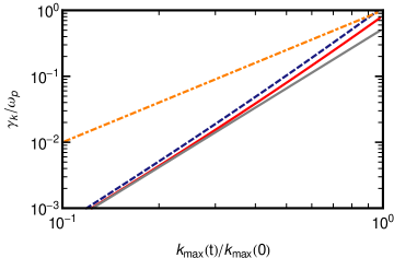
Figure 1: Damping rate vs wavenumber: in thick gray, the linear calculation; in thick red, the damping rate at first non-linear order, assuming $\kappa_{0}\,=\,1$ and $n_{B}\,=\,0$, calculated through Eq. (22); in dashed blue, the same damping rate calculated with the approximation Eq. (27); in dash-dotted orange, the scattering frequency $t_{\rm s}^{-1}$ in units of $\omega_{\rm p}$ at $\gamma_{\rm min}$.

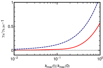
Figure 2: Evaluation of the non-linear correction to the linear damping rate ($\gamma_{k,\rm lin}$) vs wavenumber: in thick red, the correction calculated using Eq. (22); in dashed blue, the correction calculated with the approximation Eq. (27). As Fig. 1, this figure assumes $\kappa_{0}\,=\,1$ and $n_{B}\,=\,-1$.

Figure 1 also shows the evolution of the scattering frequency $t_{\rm s}^{-1}$ vs wavenumber: this allows to verify that, at all $k_{\rm max}$, one has $k^{-1}\,<\,t_{\rm s}\,<\,\gamma_{k}^{-1}$, which validates the assumptions inherent to the present approach.

These figures show that the non-linear calculation modifies the linear calculation by a factor of order unity at $k_{\rm max}(0)$, then converges to the linear calculation at smaller $k_{\rm max}$; indeed, $n_{B}\,=\,0$ implies $\kappa\,\propto\,k_{\rm max}^{-1}$: $\kappa$ increases with decreasing values of $k_{\rm max}$ at a same $\gamma_{\rm min}$, therefore the importance of non-linear effects, which is quantified by inverse powers of $\kappa$, becomes weaker as $k_{\rm max}$ decreases. As mentioned above, for $n_{B}\,=\,-1$, one would find a correction at all $k_{\rm max}$ equal to the correction calculated at $k_{\rm max}(0)$.

These calculations also indicate that the non-linear terms systematically lead to an increased damping rate, although the correction is modest. This goes contrary to the discussion in Chang et al. (2008), which conjectured that the deflection of particles by magnetic turbulence might lead to a weaker damping rate.

4 Discussion and conclusions

The present work studies the damping rate of the micro-turbulence which has been excited through e.g. Weibel/filamentation instabilities in the precursor of a weakly magnetized relativistic collisionless shock wave then transmitted downstream. As mentioned in Sec. 1, such calculations are directly relevant to the physics of collisionless shock waves, but also to high energy astrophysics, since the damping of the turbulence governs the strength of the magnetic field in which electrons radiate (and therefore the frequency at which they radiate the bulk of their energy).

In the standard afterglow model for gamma-ray burst, the canonical value for the equipartition fraction of magnetic energy density in the blast is taken as $\epsilon_{B}\,\sim\,10^{-2}$, on the basis on afterglow observations in various wavebands, see e.g. Waxman (1997), Wijers & Galama (1999) for early determinations, and Panaitescu & Kumar (2001) for a compilation of results, which however reveals a large scatter in this parameter. Such a value would fit nicely the results of PIC simulations in the absence of dissipation, since these simulations find $\epsilon_{B}\,\sim\,10^{-2}$ immediately downstream of the blast; the fact that $\epsilon_{B}$ remains that large up to the long time scales on which electrons can radiate gives rise to the notorious problem of the origin of these magnetic fields.

Recent detections of gamma-ray burst afterglows at high-energy $>100\,$MeV may have shed a new light on this issue. If this high-energy emission indeed corresponds to the synchrotron afterglow, e.g. (Kumar & Barniol Duran, 2009, 2010; Ghisellini et al., 2010), these detections offer another observational constraint to pin down $\epsilon_{B}$ beyond the degeneracies inherent to most of the previous studies, see the discussion in Lemoine et al. (2013). Then one derives low values of $\epsilon_{B}$, well below the canonical one, which may be interpreted as the partial dissipation of the Weibel-generated turbulence, as described here (Lemoine, 2013); in particular, assuming a power-law decay $\epsilon_{B}\,\propto\,(t\omega_{\rm p})^{\alpha_{t}}$ as a function of comoving time, one derives $-0.5\,\lesssim\,\alpha_{t}\,\lesssim\,-0.4$ from a handful of gamma-ray burst afterglows seen in radio, optical, X-ray and at high energy (Lemoine et al., 2013), i.e. a net dissipation. The decay of Weibel turbulence behind relativistic shock waves thus appears as a key ingredient in describing accurately the light curves of these extreme astronomical phenomena.

The present work presents a calculation of the damping rate to the first non-linear order, by computing the effects of particle diffusion in the micro-turbulence. As mentioned in Sec. 1, one interest of such a calculation is to study the dependence of this correction on the power spectrum of magnetic fluctuations, which at present cannot be reconstructed with confidence by PIC simulations. An exact calculation is possible, thanks to the small-scale and magneto-static nature of the turbulence, which allows for an explicit calculation of the trajectory correlators which determine the amount of resonance broadening. As discussed in the main text, this work assumes that the particles are not trapped in the micro-turbulence, i.e. the scattering length is assumed larger than the coherence length of the magnetic fluctuations.

The overall influence of non-linear terms is found to be of order unity at the maximum wavenumber, and to decrease with decreasing wavenumbers $k$, provided the three-dimensional power spectrum of magnetic fluctuations ${\cal S}_{\delta B}\,\propto\,k^{n_{B}}$ has an index $n_{B}\,>\,-1$. In this case, indeed, the ratio of the particle scattering timescale $t_{\rm s}$ to the coherence time $\tau_{\rm c}$ of the magnetic fluctuations increases, therefore the particle trajectories become more and more ballistic as $k$ decreases and one recovers the linear result in the small $k$ limit. The results obtained also indicate that the non-linear correction systematically increases the damping rate.

The present results would suggest that the damping rate does follow roughly the scaling $\gamma_{k}\,\propto\,k^{3}$ predicted by linear theory, however one cannot exclude at present that the power spectrum of magnetic fluctuations is such – i.e. $n_{B}\,<\,-1$ – that effects associated to particle trapping become more and more prominent as dissipation progresses (meaning, as the time-dependent maximum wavenumber decreases). Actually, if $\gamma_{k}\,\propto\,k^{\alpha_{k}}$, one can relate the decay exponent $\alpha_{t}$ to the power spectrum index $n_{B}$ and $\alpha_{k}$ (Chang et al., 2008; Lemoine, 2013):

$$\alpha_{t}\,=\,-\frac{3+n_{B}}{\alpha_{k}}\ .$$ (31)

Then, $\alpha_{k}\,\simeq\,3$ with a value $\alpha_{t}\,\sim\,-0.5$ as suggested by observations (Lemoine et al., 2013) would imply $n_{B}\,\sim\,-1.5$, in which case the ratio $t_{\rm s}/\tau_{\rm c}\,\propto\,k^{-n_{B}-1}$ would decrease with decreasing $k$: i.e., the non-linear effects would become more prominent as dissipation progresses.

The present calculations cannot address the situation in which particles are effectively trapped and other theoretical tools are needed to probe this regime and to make the connection with observations. Further PIC simulations, extended in time and dimensionality, would also provide useful guidance to better characterize the scaling of $\gamma_{k}$ vs $k$. Finally, dedicated PIC simulations with an artificially set-up power spectrum might be used to probe the regime $n_{B}\,<\,-1$ in which trapping is expected to become more effective as dissipation progresses.

It is a pleasure to thank Laurent Gremillet and Guy Pelletier for very valuable suggestions and discussions. This work has been financially supported by the “Programme National Hautes Energies” (PNHE) of the CNRS.

Appendix A

Separating the average and random parts as usual, as described in Sec. 2.2, one finds that the fluctuating part of the distribution function obeys:

$$\left[\frac{\partial}{\partial t}+{\cal L}\right]f_{\alpha}(\boldsymbol{r},\boldsymbol{p},t)-\left\langle\delta{\cal L}f_{\alpha}(\boldsymbol{r},\boldsymbol{p},t)\right\rangle\,=\,-\delta{\cal L}\overline{f}_{\alpha}$$ (32)

with:

$${\cal L}\,=\,\overline{\cal L}+\delta{\cal L},\quad\overline{\cal L}\,=\,\boldsymbol{v}\cdot\frac{\partial}{\partial\boldsymbol{r}},\quad\delta{\cal L}\,=\,q\left(\boldsymbol{\delta E}+\frac{\boldsymbol{v}}{c}\times\boldsymbol{\delta B}\right)\cdot\frac{\partial}{\partial\boldsymbol{p}}$$ (33)

Following Weinstock (1969) and Weinstock (1970), one introduces the averaging operator ${\cal A}$, which takes the average over the statistical realization of the fluctuations of all quantities to its right, i.e. $\psi_{1}(\boldsymbol{r},\boldsymbol{p},t){\cal A}\psi_{2}(\boldsymbol{r},\boldsymbol{p},t)\ldots\psi_{n}(\boldsymbol{r},\boldsymbol{p},t)\,=\,\psi_{1}\langle\psi_{2}\ldots\psi_{n}\rangle$. One then defines the following propagators:

$${\cal U}: \quad\left[\frac{\partial}{\partial t}+{\cal L}\right]{\cal U}(t,t_{0})\,=\,0,\quad{\cal U}(t_{0},t_{0})\,=\,1$$

$${\cal U_{A}}: \quad\left[\frac{\partial}{\partial t}+\left(1-{\cal A}\right){\cal L}\right]{\cal U_{A}}(t,t_{0})\,=\,0,\quad{\cal U_{A}}(t_{0},t_{0})\,=\,1$$

$${\cal\overline{U}}: \quad\left[\frac{\partial}{\partial t}+\overline{\cal L}\right]\overline{\cal U}(t,t_{0})\,=\,-\left\langle\delta{\cal L}\,{\cal U}\right\rangle,\quad\overline{\cal U}(t_{0},t_{0})\,=\,1\ .$$ (34)

${\cal U}(t,t_{0})$ of course represents the full propagator of the Vlasov equation; acting on a function $\psi(\boldsymbol{r},\boldsymbol{p},t)$, it propagates it backward in time, i.e. ${\cal U}(t,t_{0})\psi(\boldsymbol{r},\boldsymbol{p},t)\,=\,\psi(\boldsymbol{r_{s}}(t_{0}),\boldsymbol{p_{s}}(t_{0}),t_{0})$ with $\boldsymbol{r_{s}}(t_{0})$, $\boldsymbol{p_{s}}(t_{0})$ the solutions of the characteristic equations for the trajectories, such that $\boldsymbol{r_{s}}(t)=\boldsymbol{r}$ and $\boldsymbol{p_{s}}(t)=\boldsymbol{p}$. The merit of the propagator ${\cal U_{A}}$ is to provide an explicit solution for $\delta f_{\alpha}(\boldsymbol{r},\boldsymbol{p},t)$ in terms of its initial data and the average distribution function $\overline{f}_{\alpha}$.

The various propagators ${\cal U}$, ${\cal U_{A}}$ and $\overline{\cal U}$ are related through series expansions in powers of ${\cal L}$ (Birmingham & Bornatici, 1971). In order to obtain a tractable expression for ${\cal U_{A}}$, one generally truncates such series to the lowest order, which leads to ${\cal U_{A}}\,\simeq\,\overline{\cal U}$ (Dupree, 1966; Weinstock, 1969, 1970). Explicitly, one finds to the next-to-leading order (Birmingham & Bornatici, 1971):

$${\cal U}_{A}(t,t_{0})\,=\,\overline{\cal U}(t,t_{0})-\int_{t_{0}}^{t}{\rm d}\tau_{1}\,\,\overline{\cal U}(t,\tau_{1})\left(1-{\cal A}\right){\cal L}(\tau_{1})\overline{U}(\tau_{1},t_{0})\,+\ldots$$ (35)

The magnitude of the next-to-leading order term relatively to the first order term is $\tau_{\rm c}e\langle\delta B^{2}\rangle^{1/2}/(\gamma mc)$, with $\gamma$ the Lorentz factor of the particle.

The propagator $\overline{\cal U}$ acts on a function $\psi$ by propagating it backwards in time and taking the statistical average over the exact orbits:

$$\overline{\cal U}(t,t_{0})\psi(\boldsymbol{r},\boldsymbol{p},t)\,=\,\left\langle\psi\left[\boldsymbol{r_{s}}(t_{0}),\boldsymbol{p_{s}}(t_{0}),t_{0}\right]\right\rangle\ ,$$ (36)

with the boundary conditions $\boldsymbol{r_{s}}(t)=\boldsymbol{r}$ and $\boldsymbol{p_{s}}(t)=\boldsymbol{p}$. Consequently, $\overline{\cal U}$ commutes with quantities that depend solely on time.

Appendix B

This Appendix calculates the correlators over the characteristic trajectories in the turbulence, which enter the expression Eq. (20) for the non-linear susceptibility. All throughout this section, the index _s for the characteristic trajectories is dropped, for clarity.

The particle suffers pitch-angle scattering in a magnetostatic turbulence. As discussed in Plotnikov et al. (2011), a convenient way to calculate the transport coefficients is to write the time evolution of its velocity as a time-ordered product of an exponentiated Liouville operator:

$$\boldsymbol{v}(t^{\prime})\,=\,{\cal T}\,\exp\left[-\int_{t^{\prime}}^{t}{\rm d}\tau_{1}\widehat{\delta\Omega}\right]\boldsymbol{v}(t)\ ,$$ (37)

where a minus sign has been introduced in order to compute quantities at time $t^{\prime}<t$ as a function of quantities at time $t$. The rotation operator $\widehat{\delta\Omega}$ is defined as

$$\widehat{\delta\Omega}\,=\,\delta\Omega^{a}\widehat{L}_{a},\quad\delta\Omega^{a}\,=\,\frac{e\delta B^{a}}{\gamma mc}$$ (38)

with $\gamma$ the Lorentz factor of the particle, $a=1,2,3$, $\widehat{L}_{a}$ a generator of the rotation group, with matrix components: $\left.\widehat{L}_{a}\right._{k}\mbox{}^{l}\,=\,\epsilon_{ak}\mbox{}^{l}$ ($\epsilon_{akl}$ denotes the Levi-Civita symbol). Equation (37) solves the equation of motion of the particle.

The rotation operator is assumed to behave as isotropic white noise with correlation time $\tau_{\rm c}$:

$$\left\langle\delta\Omega^{a}(\tau_{1})\right\rangle\,=\,0,\quad\left\langle\delta\Omega^{a}(\tau_{1})\delta\Omega^{b}(\tau_{2})\right\rangle\,=\,\frac{2}{3}\tau_{\rm c}\delta(\tau_{1}-\tau_{2})\delta\Omega^{2}\delta^{ab}\ ,$$ (39)

with $\delta\Omega^{2}\,=\,\left[e\langle\delta B^{2}\rangle^{1/2}/(\gamma mc)\right]^{2}$. A useful identity is: $\delta^{ab}\widehat{L}_{a}\widehat{L}_{b}=-2\widehat{I}$, which implies $\left\langle\widehat{\delta\Omega}(\tau_{1})\widehat{\delta\Omega}(\tau_{2})\right\rangle\,=\,-4\delta\Omega^{2}\tau_{\rm c}\delta(\tau_{1}-\tau_{2})\widehat{I}$. Therefore, the average over the exact orbit gives

$$\left\langle\boldsymbol{v}(t^{\prime})\right\rangle\,=\,\exp\left[\frac{1}{2}\int_{t^{\prime}}^{t}{\rm d}\tau_{1}\int_{t^{\prime}}^{t}{\rm d}\tau_{2}\left\langle\widehat{\delta\Omega}(\tau_{1})\widehat{\delta\Omega}(\tau_{2})\right\rangle\right]\boldsymbol{v}\,=\,\exp\left[-\frac{2}{3}\tau_{\rm c}(t-t^{\prime})\delta\Omega^{2}\right]\boldsymbol{v}\ .$$ (40)

This correlator defines the scattering time $t_{\rm s}\,\equiv\,\frac{3}{2}\left(\tau_{\rm c}\delta\Omega^{2}\right)^{-1}$, which depends on the momentum of the particle. In the following, the generic notation $C_{a}(t)\,\equiv\,\exp\left(-at/t_{\rm s}\right)$ is adopted, with $a$ a rational number.

The calculation of the correlator $\langle v_{i}(t_{1})v_{j}(t_{2})\rangle$ is more involved as it involves the product of two time-ordered exponentials. One must stress that it differs from usual velocity correlators in diffusion calculations because of the particular boundary conditions: $v_{i}(t)=v_{i}$ and $v_{j}(t)=v_{j}$. This correlator is written:

$$v_{i}(t_{1})v_{j}(t_{2})\,=\,{\cal T}\exp\left[-\int_{t_{1}}^{t}{\rm d}\tau\,\widehat{\delta\Omega}\right]_{i}^{k}\,{\cal T}\exp\left[-\int_{t_{2}}^{t}{\rm d}\tau\,\widehat{\delta\Omega}\right]_{j}^{l}v_{k}v_{l}$$ (41)

Now, if $t_{1}>t_{2}$, one rewrites

$${\cal T}\exp\left[-\int_{t_{2}}^{t}{\rm d}\tau\,\widehat{\delta\Omega}\right]_{j}^{l}\,=\,{\cal T}\exp\left[-\int_{t_{1}}^{t}{\rm d}\tau\,\widehat{\delta\Omega}\right]_{j}^{m}\,{\cal T}\exp\left[-\int_{t_{2}}^{t_{1}}{\rm d}\tau\,\widehat{\delta\Omega}\right]_{m}^{l}$$ (42)

and conversely if $t_{2}<t_{1}$. In the following, $\overline{t}\,\equiv\,{\rm max}(t_{1},t_{2})$ and $\underline{t}\,\equiv\,{\rm min}(t_{1},t_{2})$. Furthermore, due to the white noise nature of $\widehat{\delta\Omega}$,

$$\Biggl{\langle}{\cal T} \exp\left[-\int_{\overline{t}}^{t}{\rm d}\tau\,\widehat{\delta\Omega}\right]\,{\cal T}\exp\left[-\int_{\overline{t}}^{t}{\rm d}\tau\,\widehat{\delta\Omega}\right]\,{\cal T}\exp\left[-\int_{\underline{t}}^{\overline{t}}{\rm d}\tau\,\widehat{\delta\Omega}\right]\Biggr{\rangle}\,=$$

$$\left\langle{\cal T}\exp\left[-\int_{\overline{t}}^{t}{\rm d}\tau\,\widehat{\delta\Omega}\right]\,{\cal T}\exp\left[-\int_{\overline{t}}^{t}{\rm d}\tau\,\widehat{\delta\Omega}\right]\right\rangle\,\left\langle{\cal T}\exp\left[-\int_{\underline{t}}^{\overline{t}}{\rm d}\tau\,\widehat{\delta\Omega}\right]\right\rangle$$

Finally, the action of $\left\langle{\cal T}\exp\left[-\int_{\underline{t}}^{\overline{t}}{\rm d}\tau\,\widehat{\delta\Omega}\right]\right\rangle$ on $v_{k}v_{l}$ gives a factor $C_{1}\left(\overline{t}-\underline{t}\right)v_{k}v_{l}$, see Eq. (40). One therefore needs to calculate only the first average on the r.h.s. of Eq. (LABEL:eq:avprod).

Here, a key observation is to note that the product of those two time ordered exponentials can be rewritten as the time ordered exponential of a tensorial operator; this is demonstrated in App. C. Expliciting the matrix components:

$${\cal T}\exp\left[-\int_{\overline{t}}^{t}{\rm d}\tau\,\widehat{\delta\Omega}\right]_{i}\mbox{}^{k}\,\,\,{\cal T}\exp\left[-\int_{\overline{t}}^{t}{\rm d}\tau\,\widehat{\delta\Omega}\right]_{j}\mbox{}^{l}\,=\,{\cal T}\exp\left[-\int_{\overline{t}}^{t}{\rm d}\tau\,\delta W\right]_{ij}\mbox{}^{kl}\ ,$$ (44)

with

$$\delta W_{ij}\mbox{}^{kl}\,=\,\delta W^{<}\mbox{}_{ij}\mbox{}^{kl}+\delta W^{>}\mbox{}_{ij}\mbox{}^{kl},\quad\delta W^{<}\mbox{}_{ij}\mbox{}^{kl}\,=\,\delta\Omega_{i}^{k}\,\delta_{j}^{l},\quad\delta W^{<}\mbox{}_{ij}\mbox{}^{kl}\,=\,\delta_{i}^{k}\,\delta\Omega_{j}^{l}$$ (45)

The tensor product rule in the time ordered exponential is understood as:

$$\left.\delta W\cdot\delta W\right._{ij}\mbox{}^{kl}\,\equiv\,\delta W_{ij}\mbox{}^{mn}\delta W_{mn}\mbox{}^{kl}$$ (46)

One therefore obtains:

$$\left\langle v_{i}(t_{1})v_{j}(t_{2})\right\rangle\,=\,{\cal T}\exp\left[\frac{1}{2}\int_{\overline{t}}^{t}\int_{\overline{t}}^{t}{\rm d}\tau_{1}{\rm d}\tau_{2}\left\langle\delta W(\tau_{1})\cdot\delta W(\tau_{2})\right\rangle\right]_{ij}\mbox{}^{kl}C_{1}(\overline{t}-\underline{t})v_{k}v_{l}$$ (47)

Now, using the identity

$$\left\langle\delta\Omega_{i}\mbox{}^{m}(\tau_{1})\delta\Omega_{j}\mbox{}^{n}(\tau_{2})\right\rangle \,=\, \left\langle\delta\Omega^{a}(\tau_{1})\delta\Omega^{b}(\tau_{2})\right\rangle\widehat{L_{a}}_{i}\mbox{}^{m}\widehat{L_{b}}_{j}\mbox{}^{n}$$ (48)

$$\,=\, \frac{2}{3}\tau_{\rm c}\delta(\tau_{1}-\tau_{2})\delta\Omega^{2}\left[\delta_{ij}\delta^{mn}-\delta_{i}\mbox{}^{m}\delta_{j}\mbox{}^{n}\right]$$

one finds

$$\left\langle\delta W(\tau_{1})\cdot\delta W(\tau_{2})\right\rangle_{ij}\mbox{}^{kl}\,=\,\frac{2}{3}\tau_{\rm c}\delta(\tau_{1}-\tau_{2})\delta\Omega^{2}\left[-4\delta_{i}\mbox{}^{k}\delta_{j}\mbox{}^{l}-2\delta_{i}\mbox{}^{l}\delta_{j}\mbox{}^{k}+2\delta_{ij}\delta^{kl}\right]\ .$$ (49)

This operator eventually acts on $v_{k}v_{l}$, which is symmetric in $k$ and $l$, therefore one can keep only the symmetric part. Define therefore

$$M_{ij}\mbox{}^{kl}\,=\,\delta_{i}\mbox{}^{k}\delta_{j}\mbox{}^{l}+\delta_{i}\mbox{}^{l}\delta_{j}\mbox{}^{k}-\frac{2}{3}\delta_{ij}\delta^{kl}$$ (50)

in terms of which one rewrites the symmetrized average, as indicated by the symbol $(kl)$:

$$\left\langle\delta W(\tau_{1})\cdot\delta W(\tau_{2})\right\rangle_{ij}\mbox{}^{(kl)}\,=\,-2\tau_{\rm c}\delta(\tau_{1}-\tau_{2})\delta\Omega^{2}\,M_{ij}\mbox{}^{kl}$$ (51)

Finally, the $M$ operator satisfies: $M\cdot M\,=\,2M$ so that

$$\exp(\alpha M)\,=\,1-\frac{M}{2}+e^{2\alpha}\frac{M}{2}\ ,$$ (52)

and

$$M_{ij}\mbox{}^{kl}v_{k}v_{l}\,=\,2v_{i}v_{j}-\frac{2}{3}v^{2}\delta_{ij}\ .$$ (53)

Combining together the above results, one ends up with:

$$\left\langle v_{i}(t_{1})v_{j}(t_{2})\right\rangle\,=\,C_{1}\left(\overline{t}-\underline{t}\right)\left\{C_{3}\left(t-\overline{t}\right)v_{i}v_{j}+\frac{v^{2}}{3}\delta_{ij}\left[1-C_{3}\left(t-\overline{t}\right)\right]\right\}\ ,$$ (54)

which has a simple interpretation: the correlator vanishes for time intervals $\overline{t}-\underline{t}$ larger than $t_{\rm s}$, else it tends towards $v_{i}v_{j}$ (the boundary conditions at time $t$) if $t-\overline{t}\,\ll\,t_{\rm s}/3$, or to the isotropic average $\delta_{ij}v^{2}/3$ in the opposite limit.

One then derives easily the position correlator, with $\Delta r_{i}(t^{\prime})\,\equiv\,r_{i}(t^{\prime})-r_{i}$, including the boundary condition $r_{i}(t)=r_{i}$:

$$\left\langle\Delta r_{i}(t^{\prime})\Delta r_{j}(t^{\prime})\right\rangle\, = \,\int_{t^{\prime}}^{t}\int_{t^{\prime}}^{t}{\rm d}\tau_{1}{\rm d}\tau_{2}\,\left\langle v_{i}(\tau_{1})v_{j}(\tau_{2})\right\rangle$$

$$= \,2t_{\rm s}^{2}\Biggl{\{}\left[\frac{1}{3}+\frac{1}{6}C_{3}(t-t^{\prime})-\frac{1}{2}C_{1}(t-t^{\prime})\right]v_{i}v_{j}+$$

$$\,\,\left[\frac{t-t^{\prime}}{t_{\rm s}}-\frac{4}{3}+\frac{3}{2}C_{1}(t-t^{\prime})-\frac{1}{6}C_{3}(t-t^{\prime})\right]\frac{v^{2}}{3}\delta_{ij}\Biggr{\}}$$

Similarly, one obtains

$$\left\langle\Delta r_{i}(t^{\prime})\right\rangle\,=\,-t_{\rm s}\left[1-C_{1}(t-t^{\prime})\right]v_{i}\ ,$$ (56)

hence

$$\left\langle\Delta r_{i}(t^{\prime})\Delta r_{j}(t^{\prime})\right\rangle- \left\langle\Delta r_{i}(t^{\prime})\right\rangle\left\langle\Delta r_{j}(t^{\prime})\right\rangle\,=\,$$

$$\quad\quad t_{\rm s}^{2}\Biggl{\{}\left[-\frac{1}{3}+C_{1}(t-t^{\prime})-C_{2}(t-t^{\prime})+\frac{1}{3}C_{3}(t-t^{\prime})\right]v_{i}v_{j}+$$

$$\quad\quad\quad\quad+\frac{2}{3}v^{2}\delta_{ij}\left[\frac{t-t^{\prime}}{t_{\rm s}}-\frac{4}{3}+\frac{3}{2}C_{1}(t-t^{\prime})-\frac{1}{6}C_{3}(t-t^{\prime})\right]\Biggr{\}}$$

The average $\left\langle\exp\left[i\boldsymbol{k}\cdot\boldsymbol{\Delta r}(t^{\prime})\right]\right\rangle$ can be truncated at the first cumulant, leading to

$$\left\langle\exp\left[i\boldsymbol{k}\cdot\boldsymbol{\Delta r}(t^{\prime})\right]\right\rangle\,\simeq\,\exp\Biggl{\{}ik^{i}\cdot\left\langle\Delta r_{i}(t^{\prime})\right\rangle-\frac{1}{2}k_{i}k_{j}\biggl{[}\left\langle\Delta r_{i}\Delta r_{j}\right\rangle-\left\langle\Delta r_{i}\right\rangle\left\langle\Delta r_{j}\right\rangle\biggr{]}\Biggr{\}}$$ (58)

In particular, the small-time limit $t-t^{\prime}\,\ll\,t_{\rm s}$ will be useful:

$$\left\langle\exp\left[i\boldsymbol{k}\cdot\boldsymbol{\Delta r}(t^{\prime})\right]\right\rangle\,\simeq\,\exp\left[-ikv\mu(t-t^{\prime})-\frac{1}{6}k^{2}v^{2}(1-\mu^{2})\left(t-t^{\prime}\right)^{3}/t_{\rm s}\right]\ ,$$ (59)

with $\mu=\boldsymbol{k}\boldsymbol{v}/(kv)$.

The correlator which enters the expression for the non-linear susceptibility is

$$\left\langle\exp\left[i\boldsymbol{k}\cdot\boldsymbol{\Delta r}(t^{\prime})\right]v_{j}(t^{\prime})\right\rangle\,=\,\left\langle\exp\left[i\boldsymbol{k}\cdot\boldsymbol{\Delta r}(t^{\prime})+\boldsymbol{\Delta v}\cdot\partial/\partial\boldsymbol{v}\right]\right\rangle v_{j}\ .$$ (60)

It is understood that $\boldsymbol{\Delta v}\,=\,\boldsymbol{v}(t^{\prime})-\boldsymbol{v}$ and the partial derivative $\partial/\partial\boldsymbol{v}$ does not act on $\boldsymbol{\Delta v}$. As before, the average of the exponential can be truncated at the first cumulant, leading to

$$\left\langle\exp\left[i\boldsymbol{k}\cdot\boldsymbol{\Delta r}(t^{\prime})\right]v_{j}(t^{\prime})\right\rangle \,=\,$$

$$\exp\Biggl{\{}ik^{i}\cdot\left\langle\Delta r_{i}(t^{\prime})\right\rangle-\frac{1}{2}k_{i}k_{j}\biggl{[}\left\langle\Delta r_{i}\Delta r_{j}\right\rangle-\left\langle\Delta r_{i}\right\rangle\left\langle\Delta r_{j}\right\rangle\biggr{]}+$$

$$ik_{i}\left\langle\Delta r_{i}(t^{\prime})\Delta v_{k}(t^{\prime})\right\rangle\partial/\partial v_{k}-ik_{i}\left\langle\Delta r_{i}(t^{\prime})\right\rangle\left\langle\Delta v_{k}(t^{\prime})\right\rangle\partial/\partial v_{k}\Biggr{\}}v_{j}$$

where the second-order cumulant $\langle\Delta v_{j}\Delta v_{k}\rangle\partial/\partial v_{j}\partial/\partial v_{k}$ has not been considered because it vanishes when acting on $\boldsymbol{v}$. Expanding the exponential in $\partial/\partial v_{j}$ to first order, one ends up with

$$\left\langle\exp\left[i\boldsymbol{k}\cdot\boldsymbol{\Delta r}(t^{\prime})\right]v_{j}(t^{\prime})\right\rangle \,=\, \left\langle\exp\left[i\boldsymbol{k}\cdot\boldsymbol{\Delta r}(t^{\prime})\right]\right\rangle$$ (62)

$$\quad\quad\times\Biggl{\{}\langle v_{j}\rangle+ik_{i}\biggl{[}\left\langle\Delta r_{i}(t^{\prime})\Delta v_{j}(t^{\prime})\right\rangle-\left\langle\Delta r_{i}(t^{\prime})\right\rangle\left\langle\Delta v_{j}(t^{\prime})\right\rangle\biggr{]}\Biggr{\}}$$

$$\,=\, \left\langle\exp\left[i\boldsymbol{k}\cdot\boldsymbol{\Delta r}(t^{\prime})\right]\right\rangle\Biggl{\{}C_{1}(t-t^{\prime})v_{j}+$$

$$\quad\quad ikvt_{\rm s}\mu\left[\frac{1}{2}C_{1}(t-t^{\prime})-C_{2}(t-t^{\prime})+\frac{1}{2}C_{3}(t-t^{\prime})\right]v_{j}-$$

$$\quad\quad\frac{i}{3}k_{j}v^{2}t_{\rm s}\left[1-\frac{3}{2}C_{1}(t-t^{\prime})+\frac{1}{2}C_{3}(t-t^{\prime})\right]\Biggr{\}}$$

In calculating the transverse susceptibility, the (longitudinal) last term $\propto k_{j}$ disappears, of course.

Appendix C

In order to demonstrate Eq. (44), one needs to expand the time ordered exponentials. The left hand side reads

$${\cal T}\exp\left[-\int_{\overline{t}}^{t}{\rm d}\tau\,\widehat{\delta\Omega}\right]_{i}^{k} \,{\cal T}\exp\left[-\int_{\overline{t}}^{t}{\rm d}\tau\,\widehat{\delta\Omega}\right]_{j}^{l}\,=\,\sum_{m,n=0}^{+\infty}\frac{1}{m!\,n!}\,$$

$$\overbrace{\int_{\overline{t}}^{t}{\rm d}\tau_{1}\,\delta\Omega_{i_{1}}^{i_{2}}\int_{\overline{t}}^{\tau_{1}}{\rm d}\tau_{2}\,\delta\Omega_{i_{2}}^{i_{3}}\ldots}^{m\,{\rm arguments}}\overbrace{\int_{\overline{t}}^{t}{\rm d}\tau^{\prime}_{1}\,\delta\Omega_{j_{1}}^{j_{2}}\int_{\overline{t}}^{\tau^{\prime}_{1}}{\rm d}\tau^{\prime}_{2}\,\delta\Omega_{j_{2}}^{j_{3}}\ldots}^{n\,{\rm arguments}}$$

and it is understood that $i_{1}=i$, $i_{m+1}=k$, $j_{1}=j$, $j_{n+1}=l$. The product of the $m$ by $n$ integrals can be written as a single time ordered sequence as follows. For the sake of clarity, one first rewrites $\delta\Omega^{<}$ the operators with $i$ indices and $\delta\Omega^{>}$ the operators with $j$ indices and one keeps in mind that all $\delta\Omega^{<}$ operators are contracted one with the other according to the time ordered sequence, and similarly for the $\delta\Omega^{>}$ operators. Then, one breaks the integral $\int_{\overline{t}}^{t}{\rm d}\tau^{\prime}_{1}\delta\Omega^{>}_{j_{1}}\mbox{}^{j_{2}}$ over the time intervals $[\overline{t},\tau_{m}]$, $[\tau_{m},\tau_{m-1}]$,…$[\tau_{1},t]$ and one reorders the sequence, noting that (indices discarded):

$$\int_{\overline{t}}^{\tau_{i}}{\rm d}\tau_{i+1}\,\delta\Omega^{<}\int_{\tau_{i+1}}^{\tau_{i}}{\rm d}\tau_{j}\,\delta\Omega^{>}\,=\,\int_{\overline{t}}^{\tau_{i}}{\rm d}\tau_{j}\,\delta\Omega^{>}\int_{\overline{t}}^{\tau_{j}}{\rm d}\tau_{i+1}\,\delta\Omega^{<}.$$ (64)

Repeating this exercise for all $\delta\Omega^{>}$ integrals, in the order of the time sequence, one ends up with a time ordered sum over all possible permutations $\sigma_{mn}$ of the operators:

$${\cal T}\exp\left[-\int_{\overline{t}}^{t}{\rm d}\tau\,\widehat{\delta\Omega}\right]_{i}^{k} \,{\cal T}\exp\left[-\int_{\overline{t}}^{t}{\rm d}\tau\,\widehat{\delta\Omega}\right]_{j}^{l}\,=\,\sum_{m,n=0}^{+\infty}\frac{1}{m!\,n!}\,\sum_{\sigma_{mn}}$$

$$\int_{\overline{t}}^{t}{\rm d}\tau_{1}\,\delta\Omega^{\sigma_{mn}(1)}\int_{\overline{t}}^{\tau_{1}}{\rm d}\tau_{2}\,\delta\Omega^{\sigma_{mn}(2)}\ldots\int_{\overline{t}}^{\tau_{m+n}}{\rm d}\tau_{m+n}\,\delta\Omega^{\sigma_{mn}(m+n)}\ .$$

The permutation is defined by: $\sigma_{mn}(a)\,=\,\left(>\,{\rm or}\,<\right)$, with $m$ copies of $<$ and $n$ copies of $>$. The indices have been discarded, but it is understood that all operators are contracted within their respective $<$ or $>$ families, as mentioned previously. One then notes that this contraction sequence can be rewritten as the tensor product of $\delta W^{<},\,\delta W^{>}$ operators introduced above, namely:

$$\left[\delta\Omega^{\sigma_{mn}(1)}\delta\Omega^{\sigma_{mn}(2)}\ldots\delta\Omega^{\sigma_{mn}(m+n)}\right]\mbox{}_{ij}\mbox{}^{kl}\,=\,\left[\delta W^{\sigma_{mn}(1)}\cdot\delta W^{\sigma_{mn}(2)}\cdot\ldots\cdot\delta W^{\sigma_{mn}(m+n)}\right]\mbox{}_{ij}\mbox{}^{kl}$$ (66)

since $\delta W^{<}$ acts non-trivially only on $i-$type indices, while $\delta W^{>}$ acts non-trivially only on $j-$type indices.

Finally, one uses:

$$\sum_{m,n=0}^{+\infty}\frac{1}{m!\,n!}\,{\cal T}\int{\rm d}\tau_{1}\,\delta W^{\sigma_{mn}(1)} \int{\rm d}\tau_{2}\,\delta W^{\sigma_{mn}(2)}\,\ldots\,=\,\sum_{p=0}^{\infty}\frac{1}{p!}\sum_{m=0}^{p}\frac{p!}{m!\,(p-m)!}$$

$${\cal T}\int{\rm d}\tau_{1}\,\delta W^{\sigma_{m,p-m}(1)}\int{\rm d}\tau_{2}\,\delta W^{\sigma_{m,p-m}(2)}\ldots$$

to obtain

$${\cal T}\exp\left[-\int_{\overline{t}}^{t}{\rm d}\tau\,\widehat{\delta\Omega}\right]_{i}^{k}\,{\cal T}\exp\left[-\int_{\overline{t}}^{t}{\rm d}\tau\,\widehat{\delta\Omega}\right]_{j}^{l}\,=\,\sum_{p=0}^{\infty}\frac{1}{p!}\,{\cal T}\left[\int_{\underline{t}}^{\overline{t}}{\rm d}\tau\left(\delta W^{<}+\delta W^{>}\right)\right]^{p}\mbox{}_{ij}\mbox{}^{kl}$$ (68)

which gives the desired result.

References

• Achterberg et al. (2001) Achterberg, A., Gallant, Y. A., Kirk, J. G. & Guthmann, A. W. 2001 Particle acceleration by ultrarelativistic shocks: theory and simulations. MNRAS 328, 393–408.
• Achterberg & Wiersma (2007) Achterberg, A. & Wiersma, J. 2007 The Weibel instability in relativistic plasmas. I. Linear theory. Astron. Astrophys. 475, 1–18.
• Achterberg et al. (2007) Achterberg, A., Wiersma, J. & Norman, C. A. 2007 The Weibel instability in relativistic plasmas. II. Nonlinear theory and stabilization mechanism. Astron. Astrophys. 475, 19–36.
• Bednarz & Ostrowski (1998) Bednarz, J. & Ostrowski, M. 1998 Energy Spectra of Cosmic Rays Accelerated at Ultrarelativistic Shock Waves. Physical Review Letters 80, 3911–3914.
• Ben-Israel et al. (1975) Ben-Israel, I., Piran, T., Eviatar, A. & Weinstock, J. 1975 A statistical theory of electromagnetic waves in turbulent plasmas. Astrophys. Sp. Sc. 38, 125–155.
• Bergman & Eliasson (2001) Bergman, J. & Eliasson, B. 2001 Linear wave dispersion laws in unmagnetized relativistic plasma: Analytical and numerical results. Physics of Plasmas 8, 1482–1492.
• Bezzerides & Weinstock (1972) Bezzerides, B. & Weinstock, J. 1972 Nonlinear Saturation of Parametric Instabilities. Physical Review Letters 28, 481–484.
• Birmingham & Bornatici (1971) Birmingham, T. J. & Bornatici, M. 1971 Propagators in Strong Plasma Turbulence. Physics of Fluids 14, 2239–2241.
• Blandford & Eichler (1987) Blandford, R. & Eichler, D. 1987 Particle acceleration at astrophysical shocks: A theory of cosmic ray origin. Phys. Rep. 154, 1–75.
• Blandford & McKee (1976) Blandford, R. D. & McKee, C. F. 1976 Fluid dynamics of relativistic blast waves. Physics of Fluids 19, 1130–1138.
• Bret et al. (2010) Bret, A., Gremillet, L. & Dieckmann, M. E. 2010 Multidimensional electron beam-plasma instabilities in the relativistic regime. Physics of Plasmas 17 (12), 120501.
• Chang et al. (2008) Chang, P., Spitkovsky, A. & Arons, J. 2008 Long-Term Evolution of Magnetic Turbulence in Relativistic Collisionless Shocks: Electron-Positron Plasmas. ApJ 674, 378–387.
• Drake & Gregori (2012) Drake, R. P. & Gregori, G. 2012 Design Considerations for Unmagnetized Collisionless-shock Measurements in Homologous Flows. Astrophys. J. 749, 171.
• Dum & Dupree (1970) Dum, C. T. & Dupree, T. H. 1970 Nonlinear Stabilization of High-Frequency Instabilities in a Magnetic Field. Physics of Fluids 13, 2064–2081.
• Dupree (1966) Dupree, T. H. 1966 A Perturbation Theory for Strong Plasma Turbulence. Physics of Fluids 9, 1773–1782.
• Felten & Schlickeiser (2013a) Felten, T. & Schlickeiser, R. 2013a Spontaneous electromagnetic fluctuations in unmagnetized plasmas. V. Relativistic form factors of weakly damped/amplified thermal modes. Physics of Plasmas 20 (8), 082117.
• Felten & Schlickeiser (2013b) Felten, T. & Schlickeiser, R. 2013b Spontaneous electromagnetic fluctuations in unmagnetized plasmas. VI. Transverse, collective mode for arbitrary distribution functions. Physics of Plasmas 20 (10), 104502.
• Felten et al. (2013) Felten, T., Schlickeiser, R., Yoon, P. H. & Lazar, M. 2013 Spontaneous electromagnetic fluctuations in unmagnetized plasmas. II. Relativistic form factors of aperiodic thermal modes. Physics of Plasmas 20 (5), 052113.
• Ghisellini et al. (2010) Ghisellini, G., Ghirlanda, G., Nava, L. & Celotti, A. 2010 GeV emission from gamma-ray bursts: a radiative fireball? Month. Not. Roy. Astron. Soc. 403, 926–937.
• Gruzinov (2000) Gruzinov, A. 2000 Ultra-Relativistic Blast Wave: Stability and Strong Non-Universality. ArXiv Astrophysics e-prints .
• Gruzinov & Waxman (1999) Gruzinov, A. & Waxman, E. 1999 Gamma-Ray Burst Afterglow: Polarization and Analytic Light Curves. Astrophys. J. 511, 852–861.
• Kato & Takabe (2008) Kato, T. N. & Takabe, H. 2008 Nonrelativistic Collisionless Shocks in Unmagnetized Electron-Ion Plasmas. ApJL 681, L93–L96.
• Katz et al. (2007) Katz, B., Keshet, U. & Waxman, E. 2007 Self-Similar Collisionless Shocks. Astrophys. J. 655, 375–390.
• Kelner et al. (2013) Kelner, S. R., Aharonian, F. A. & Khangulyan, D. 2013 On the Jitter Radiation. Astrophys. J. 774, 61.
• Keshet et al. (2009) Keshet, U., Katz, B., Spitkovsky, A. & Waxman, E. 2009 Magnetic Field Evolution in Relativistic Unmagnetized Collisionless Shocks. ApJL 693, L127–L130.
• Keshet & Waxman (2005) Keshet, U. & Waxman, E. 2005 Energy Spectrum of Particles Accelerated in Relativistic Collisionless Shocks. Physical Review Letters 94 (11), 111102.
• Kirk et al. (2000) Kirk, J. G., Guthmann, A. W., Gallant, Y. A. & Achterberg, A. 2000 Particle Acceleration at Ultrarelativistic Shocks: An Eigenfunction Method. Astrophys. J. 542, 235–242.
• Kocharovsky et al. (2010) Kocharovsky, V. V., Kocharovsky, V. V. & Martyanov, V. J. 2010 Self-Consistent Current Sheets and Filaments in Relativistic Collisionless Plasma with Arbitrary Energy Distribution of Particles. Physical Review Letters 104 (21), 215002.
• Kumar & Barniol Duran (2009) Kumar, P. & Barniol Duran, R. 2009 On the generation of high-energy photons detected by the Fermi Satellite from gamma-ray bursts. Month. Not. Roy. Astron. Soc. 400, L75–L79.
• Kumar & Barniol Duran (2010) Kumar, P. & Barniol Duran, R. 2010 External forward shock origin of high-energy emission for three gamma-ray bursts detected by Fermi. Month. Not. Roy. Astron. Soc. 409, 226–236.
• Lemoine (2013) Lemoine, M. 2013 Synchrotron signature of a relativistic blast wave with decaying microturbulence. MNRAS 428, 845–866.
• Lemoine et al. (2013) Lemoine, M., Li, Z. & Wang, X.-Y. 2013 On the magnetization of gamma-ray burst blast waves. Month. Not. Roy. Astron. Soc. 435, 3009–3016.
• Lemoine & Pelletier (2003) Lemoine, M. & Pelletier, G. 2003 Particle Transport in Tangled Magnetic Fields and Fermi Acceleration at Relativistic Shocks. Astrophys. J. 589, L73–L76.
• Lemoine & Pelletier (2010) Lemoine, M. & Pelletier, G. 2010 On electromagnetic instabilities at ultra-relativistic shock waves. MNRAS 402, 321–334.
• Lemoine & Pelletier (2011) Lemoine, M. & Pelletier, G. 2011 Dispersion and thermal effects on electromagnetic instabilities in the precursor of relativistic shocks. MNRAS 417, 1148–1161.
• Lemoine et al. (2006) Lemoine, M., Pelletier, G. & Revenu, B. 2006 On the Efficiency of Fermi Acceleration at Relativistic Shocks. Astrophys. J. Lett. 645, L129–L132.
• Levinson (2009) Levinson, A. 2009 Convective Instability of a Relativistic Ejecta Decelerated by a Surrounding Medium: An Origin of Magnetic Fields in Gamma-Ray Bursts? Astrophys. J.l 705, L213–L216.
• Levinson (2010) Levinson, A. 2010 Relativistic Rayleigh-Taylor instability of a decelerating shell and its implications for gamma-ray bursts. Geophysical and Astrophysical Fluid Dynamics 104, 85–111.
• Lyubarsky & Eichler (2006) Lyubarsky, Y. & Eichler, D. 2006 Are Gamma-Ray Burst Shocks Mediated by the Weibel Instability? ApJ 647, 1250–1254.
• Mart’yanov et al. (2008) Mart’yanov, V. Y., Kocharovsky, V. V. & Kocharovsky, V. V. 2008 Saturation of relativistic Weibel instability and the formation of stationary current sheets in collisionless plasma. Soviet Journal of Experimental and Theoretical Physics 107, 1049–1060.
• Medvedev et al. (2005) Medvedev, M. V., Fiore, M., Fonseca, R. A., Silva, L. O. & Mori, W. B. 2005 Long-Time Evolution of Magnetic Fields in Relativistic Gamma-Ray Burst Shocks. Astrophys. J. 618, L75–L78.
• Medvedev et al. (2011) Medvedev, M. V., Frederiksen, J. T., Haugbølle, T. & Nordlund, Å. 2011 Radiation Signatures of Sub-Larmor Scale Magnetic Fields. Astrophys. J. 737, 55.
• Medvedev & Loeb (1999) Medvedev, M. V. & Loeb, A. 1999 Generation of Magnetic Fields in the Relativistic Shock of Gamma-Ray Burst Sources. ApJ 526, 697–706.
• Medvedev & Zakutnyaya (2009) Medvedev, M. V. & Zakutnyaya, O. V. 2009 Magnetic Fields and Cosmic Rays in GRBs: A Self-Similar Collisionless Foreshock. Astrophys. J. 696, 2269–2274.
• Mizuno et al. (2014) Mizuno, Y., Pohl, M., Niemiec, J., Zhang, B., Nishikawa, K.-I. & Hardee, P. E. 2014 Magnetic field amplification and saturation in turbulence behind a relativistic shock. Month. Not. Roy. Astron. Soc. 439, 3490–3503.
• Moiseev & Sagdeev (1963) Moiseev, S. S. & Sagdeev, R. Z. 1963 Collisionless shock waves in a plasma in a weak magnetic field. Journal of Nuclear Energy 5, 43–47.
• Niemiec et al. (2006) Niemiec, J., Ostrowski, M. & Pohl, M. 2006 Cosmic-Ray Acceleration at Ultrarelativistic Shock Waves: Effects of Downstream Short-Wave Turbulence. ApJ 650, 1020–1027.
• Panaitescu & Kumar (2001) Panaitescu, A. & Kumar, P. 2001 Fundamental Physical Parameters of Collimated Gamma-Ray Burst Afterglows. Astrophys. J.l 560, L49–L53.
• Pelletier (1977) Pelletier, G. 1977 Renormalization method and singularities in the theory of Langmuir turbulence. Journal of Plasma Physics 18, 49–76.
• Pelletier et al. (2009) Pelletier, G., Lemoine, M. & Marcowith, A. 2009 On Fermi acceleration and magnetohydrodynamic instabilities at ultra-relativistic magnetized shock waves. MNRAS 393, 587–597.
• Piran (2004) Piran, T. 2004 The physics of gamma-ray bursts. Rev. Mod. Phys. 76, 1143–1210.
• Plotnikov et al. (2011) Plotnikov, I., Pelletier, G. & Lemoine, M. 2011 Particle transport in intense small-scale magnetic turbulence with a mean field. Astron. Astrophys. 532, A68.
• Pokhotelov & Amariutei (2011) Pokhotelov, O. A. & Amariutei, O. A. 2011 Quasi-linear dynamics of Weibel instability. Annales Geophysicae 29, 1997–2001.
• Rabinak et al. (2011) Rabinak, I., Katz, B. & Waxman, E. 2011 Long-wavelength Unstable Modes in the Far Upstream of Relativistic Collisionless Shocks. ApJ 736, 157.
• Ruyer et al. (2013) Ruyer, C., Gremillet, L., Bénisti, D. & Bonnaud, G. 2013 Electromagnetic fluctuations and normal modes of a drifting relativistic plasma. Physics of Plasmas 20 (11), 112104.
• Shaisultanov et al. (2012) Shaisultanov, R., Lyubarsky, Y. & Eichler, D. 2012 Stream Instabilities in Relativistically Hot Plasma. ApJ 744, 182.
• Sironi & Goodman (2007) Sironi, L. & Goodman, J. 2007 Production of Magnetic Energy by Macroscopic Turbulence in GRB Afterglows. Astrophys. J. 671, 1858–1867.
• Sironi & Spitkovsky (2009) Sironi, L. & Spitkovsky, A. 2009 Synthetic Spectra from Particle-In-Cell Simulations of Relativistic Collisionless Shocks. Astrophys. J. Lett. 707, L92–L96.
• Sironi et al. (2013) Sironi, L., Spitkovsky, A. & Arons, J. 2013 The Maximum Energy of Accelerated Particles in Relativistic Collisionless Shocks. ApJ 771, 54.
• Spitkovsky (2008a) Spitkovsky, A. 2008a On the Structure of Relativistic Collisionless Shocks in Electron-Ion Plasmas. ApJL 673, L39–L42.
• Spitkovsky (2008b) Spitkovsky, A. 2008b Particle Acceleration in Relativistic Collisionless Shocks: Fermi Process at Last? ApJL 682, L5–L8.
• Waxman (1997) Waxman, E. 1997 Gamma-Ray–Burst Afterglow: Supporting the Cosmological Fireball Model, Constraining Parameters, and Making Predictions. Astrophys. J.l 485, L5–L8.
• Weinstock (1969) Weinstock, J. 1969 Formulation of a Statistical Theory of Strong Plasma Turbulence. Physics of Fluids 12, 1045–1058.
• Weinstock (1970) Weinstock, J. 1970 Turbulent Plasmas in a Magnetic Field-A Statistical Theory. Physics of Fluids 13, 2308–2316.
• Weinstock (1972) Weinstock, J. 1972 Nonlinear Theory of Frequency Shifts and Broadening of Plasma Waves. Physics of Fluids 15, 454–459.
• Weinstock & Bezzerides (1973) Weinstock, J. & Bezzerides, B. 1973 Nonlinear saturation of parametric instabilities: Spectrum of turbulence and enhanced collision frequency. Physics of Fluids 16, 2287–2303.
• Wiersma & Achterberg (2004) Wiersma, J. & Achterberg, A. 2004 Magnetic field generation in relativistic shocks. An early end of the exponential Weibel instability in electron-proton plasmas. Astron. Astrophys. 428, 365–371.
• Wijers & Galama (1999) Wijers, R. A. M. J. & Galama, T. J. 1999 Physical Parameters of GRB 970508 and GRB 971214 from Their Afterglow Synchrotron Emission. Astrophys. J. 523, 177–186.
• Yoon et al. (2014) Yoon, P. H., Schlickeiser, R. & Kolberg, U. 2014 Thermal fluctuation levels of magnetic and electric fields in unmagnetized plasma: The rigorous relativistic kinetic theory. Physics of Plasmas 21 (3), 032109.