Slow ionized wind and rotating disklike system associated with the high-mass young stellar object G345.4938+01.4677

Abstract

We report the detection, made using ALMA, of the 92 GHz continuum and hydrogen recombination lines (HRLs) H40$\alpha$, H42$\alpha$, and H50$\beta$ emission toward the ionized wind associated with the high-mass young stellar object G345.4938+01.4677. This is the luminous central dominating source located in the massive and dense molecular clump associated with IRAS 16562$-$3959. The HRLs exhibit Voigt profiles, a strong signature of Stark broadening. We successfully reproduce the observed continuum and HRLs simultaneously using a simple model of a slow ionized wind in local thermodynamic equilibrium, with no need a high-velocity component. The Lorentzian line wings imply electron densities of $5\times 10^{7}$ cm^-3 on average. In addition, we detect SO and SO₂ emission arising from a compact ($\sim 3000$ AU) molecular core associated with the central young star. The molecular core exhibits a velocity gradient perpendicular to the jet-axis, which we interpret as evidence of rotation. The set of observations toward G345.4938+01.4677 are consistent with it being a young high-mass star associated with a slow photo-ionized wind.

1 INTRODUCTION

Stars of all masses form by gravitational collapse within unstable regions of molecular clouds. Observationally, low-mass star formation is characterized by the following inter-related phenomena: an infalling envelope, an accretion disk, and a highly collimated jet (Shu et al., 1987; Li et al., 2014). Highly collimated jets, flowing outwards in a roughly symmetrical fashion are one of the most spectacular phenomena occurring during the formation of stars (De Young, 1991). The origin and driving mechanism of these stellar jets are still major open issues, although the presence of an accretion disk (Livio, 2009) and magnetic fields are thought to be key in explaining the efficient jet acceleration and collimation (Blandford & Payne, 1982; Cabrit, 2007). There is a jet-disk symbiosis, well established observationally in the case of low-mass protostars, by which the surrounding accretion disk feeds the jet by transporting gas and dust from the infalling envelope to the protostar and the jet removes angular momentum and magnetic flux from the disk allowing accretion to proceed (Frank et al., 2014).

High-mass stars ($M_{\star}>8\mbox{$\,M_{\sun}$}$) form by accretion within massive ($\sim 10^{3}\mbox{$\,M_{\sun}$}$) and dense ($10^{4\text{-}5}$ cm^-3) molecular clumps, with typical diameters of 1 pc and generally supported by turbulent motions (Garay, 2005; Zinnecker & Yorke, 2007; Tan et al., 2014). These clumps harbor the luminous embedded infrared sources known as high-mass young stellar objects (HMYSOs), that represent an early evolutionary stage of a single high-mass star or a multiple stellar system. It is probable, also, that some high-mass stars are born forming tight binary systems that will eventually merge, populating the highest end of the stellar mass spectrum (Sana et al., 2012). Toward some massive clumps, the following phenomena — analogous to the ones observed in low-mass star formation — are detected:

• Extended infalling envelopes, with inflows motions involving a sizable fraction of the molecular clump (Ho & Haschick, 1986; Zhang & Ho, 1997; Garay et al., 2002, 2003; Wu & Evans, 2003).

• Bipolar molecular outflows, which are poorly collimated but much more massive and energetic than in the low-mass case (Zhang et al., 2001; Beuther et al., 2002; Wu et al., 2004; Zhang et al., 2005; Beltrán et al., 2011).

• Rotation-flattened molecular structures surrounding the HMYSOs, ranging from transient toroids with sizes $\geq 5000$ AU (Zhang, 2005; Beltrán et al., 2006) to more stable, disklike structures of $500$-$2000$ AU where centrifugal support may play a role (Patel et al., 2005; Franco-Hernández et al., 2009; Qiu et al., 2012; Sánchez-Monge et al., 2013; Beuther et al., 2013; Hunter et al., 2014).

When both bipolar outflows and rotating molecular structures are detected, the symmetry axis of the former and the velocity gradient of the latter are usually perpendicular. Most disklike structures around HMYSOs are, however, considerably different compared to low-mass circumstellar disks: they are not thin or supported entirely by rotation, and they might be unstable to further fragmentation. The closest analogs to low-mass circumstellar disks are the ones discovered around HMYSOs that are not deeply embedded (e.g., Kraus et al., 2010; Fallscheer et al., 2011). In addition, young high-mass stars emit copious amounts of UV radiation that ionize their surroundings (Keto & Wood, 2006; Keto & Klaassen, 2008). Important unsettled questions are: Does the infall extend all the way to the molecular core? Do accretion disks exist within rotating cores? Are molecular outflows driven by underlying collimated jets powered by accretion? Numerical models have shown that disks (e.g., Kuiper et al., 2011) and jets (e.g., Vaidya et al., 2011) are theoretically possible to form and sustain around young high-mass stars.

Optical and radio continuum observations indicate that a fraction of the matter in the young stellar jet is in the form of ionized gas (Anglada, 1996), i.e., the ionized jet. Examples of ionized jets associated to HMYSOs observed in radio continuum are IRAS 18162$-$2048 (also HH 80-81, Martí et al., 1993), Cepheus A HW2 (Rodríguez et al., 1994), IRAS 20126+4104 (Tofani et al., 1995; Cesaroni et al., 1997), G192.16$-$3.82 (Shepherd et al., 1998), W75N VLA 3 (Carrasco-González et al., 2010), AFGL 2591 VLA 3 (Johnston et al., 2013), G35.2$-$0.7N (Gibb et al., 2003), NGC7538 IRS 1 (Sandell et al., 2009), G343.1262$-$00.0620 (Garay et al., 2003, 2007, also IRAS 16547$-$4247), and G345.4938+01.4677 (Guzmán et al., 2010, 2011, also IRAS 16562$-$3959). Most of the present knowledge about ionized jets comes from studies at optical and near-infrared (NIR) wavelengths of low-mass young stars still associated with their protostellar disks, but no longer embedded in their parental molecular cores, referred to as Class II objects (Ray et al., 2007). Young stars in earlier evolutionary phases are still deeply embedded within their parental cores of dust and gas and are thus undetectable at optical or NIR observations. This is the general situation in jets associated with high-mass stars. Radio continuum observations, on the other hand, are not affected by dust absorption and are able to probe the characteristics of deeply embedded ionized jets.

Physical parameters of ionized jets associated with high-mass stars, such as the degree of collimation, ionization fraction, or kinematics, are not well determined, and they are usually constrained from observations of the lobes. In particular, estimates of the velocity of the gas in the jet are derived from measurements of the lobes proper motion. In most cases, the estimates are close to $\sim$500 km s^-1(Martí et al., 1998; Curiel et al., 2006; Rodríguez et al., 2008), considerably faster than the jet velocity of their low-mass counterparts. The dominant assumption in the literature has been that the velocity of the ionized gas within the jet is similar to that of the lobes. Until now, the only direct observational support for this assumption has been provided by hydrogen recombination line (HRL) observations made by Jiménez-Serra et al. (2011) toward the B-type YSO Cepheus A HW2. While HRLs have become standard tools to study regions of ionized gas (Mezger & Palmer, 1968; Brown et al., 1978; Gordon & Sorochenko, 2002), this has not been true for jets, which have much weaker flux densities and smaller sizes than classical H ii regions.

We present ALMA Band-3 observations of the HMYSO G345.4938+01.4677 (also IRAS 16562$-$3959). This HMYSO is associated with an ionized wind and symmetrically located lobes detected in centimeter radio continuum by Guzmán et al. (2010), an infalling envelope, and a bipolar molecular outflow (Guzmán et al., 2010, 2011). In the following, we use the name IRAS 16562$-$3959 to refer to the more extended, $\sim 40\arcsec$ angular size molecular clump characterized by single dish observations (e.g., Faúndez et al., 2004). G345.4938+01.4677 (G345.49+1.47 hereafter) is then the central dominating HMYSO within IRAS 16562$-$3959. For the present work, we adopt a distance to IRAS 16562$-$3959 of 1.7 kpc (López et al., 2011). The gas mass of IRAS 16562$-$3959 is $\sim 900\mbox{$\,M_{\sun}$}$. Assuming that approximately 30% of this mass will end up as stellar mass in a cluster (Lada & Lada, 2003), and using the empirical relationship $M_{\rm max}=1.2M_{\rm cluster}^{0.45}$ where $M_{\rm max}$ is the mass of the most massive member of a cluster and $M_{\rm cluster}$ is the cluster’s mass (in units of solar mass, see Larson, 2003), we determine that the likely mass of the central star of G345.49+1.47 is $\sim 15\mbox{$\,M_{\sun}$}$. In this work, we focus on results derived from the continuum, HRLs, and sulfuretted molecular lines, and we leave the analysis of other observed molecular tracers (e.g., SiO, CH₃OH, and C₂H) for upcoming publications.

Section 2 presents the ALMA observations toward G345.49+1.47 and data reduction. Section 3 presents the results from the radio continuum, from the three HRLs, and from the sulfuretted molecules. We discuss and model the results in Section 4, where we suggest that the G345.49+1.47 radio continuum and HRL emission are best explained as arising from a photo-ionized disk wind. Section 5 summarizes our main conclusions.

2 OBSERVATIONS

Table 1: Spectral Setting and Angular Resolution

	85.4 GHz	87.2 GHz	97.6 GHz	99.3 GHz
Spectral Window Limits (GHz)	[84.42, 86.30]	[86.18, 88.06]	[96.68, 98.56]	[98.38, 100.26]
Synthesized Beams	2.51″$\times$1.42″	2.47″$\times$1.40″	2.22″$\times$1.24″	2.18″$\times$1.26″
Position Angle	$97.8\arcdeg$	$97.3\arcdeg$	$97.2\arcdeg$	$97.7\arcdeg$

Data were obtained using the Atacama Large Millimeter/sub-millimeter Array (ALMA) during Cycle 0 using the extended array configuration (longest and shortest baselines 453 and 21 m, respectively). We observed G345.49+1.47 for $\sim$188 minutes on-source in Band-3, which covers the 3 mm atmospheric window, in 5 scheduling blocks. Two scheduling blocks were observed with 17 12-m antennas, and the other three with 25. The phase center of the array was R.A.$=16^{\rm h}59^{\rm m}$41$\fs$63, decl.$=-$40°03′43$\farcs$61 (J2000), the position of the central jet source identified by Guzmán et al. (2010).

The observations covered four spectral windows (SpWs), each one spanning 1.875 GHz. Each SpW consisted of 3840 channels of 488 kHz width and were centered at 85.4, 87.2, 97.6, and 99.3 GHz. We use these frequencies to refer to each SpW throughout this work. The effective spectral resolution is approximately two times the channel width, that is 976 kHz, which corresponds to $\sim$3.0 km s^-1. Table 1 gives the spectral limits of each SpW, and the synthesized beam of the array at these frequencies, which was typically $2\farcs 3\times 1\farcs 3$ with a position angle of 97° (Table 1). The primary beam FWHM was $67$″, and the typical system temperature was $70$ K.

We recalibrated the data using the Common Astronomy Software Applications (CASA) (v.4.0.1 Petry & CASA Development Team, 2012). The sources Neptune and Titan were used as flux calibrators, J1924$-$292 and 3C279 were used as bandpass calibrators, and J1717$-$337 was used as a gain calibrator. The flux densities derived for J1717$-$337 were $1.46\pm 0.03$, $1.44\pm 0.03$, $1.37\pm 0.03$, and $1.36\pm 0.03$ Jy at 85.4, 87.2, 97.6, and 99.3 GHz, respectively.

Maps were generated by Fourier transformation of the robust-weighted visibilities (Briggs, 1995), robust parameter $=0$, and deconvolved using the clean task within CASA. The pixel size used was $0\farcs 3\times 0\farcs 3$ in all cases. Most of the flux density detected toward G345.49+1.47 arises from a compact continuum source of $\sim 0.1$ Jy, which allowed us to perform an additional phase self-calibration iteration. All visibilities were calibrated in phase using this self-calibrated solution.

The spectral location of HRLs and strong molecular lines was masked out by visual inspection to isolate the continuum emission. This continuum was subtracted from the visibility data using the CASA task uvcontsub. The noise level achieved in the continuum maps for each SpW was typically 50 $\mu$Jy beam^-1, as measured by the rms of the final images. Deconvolved images per channel were obtained for selected spectral lines using clean, achieving noise levels of 1-2 mJy beam^-1. The continuum and spectral cube noise levels attained are comparable to the theoretical sensitivity calculated using the ALMA Observing Tool, which indicates 25 $\mu$Jy per SpW for the continuum and 1.4 mJy per channel for the spectral lines.

Fully reduced datasets, continuum, and spectral cubes are publicly available through the Dataverse.

3 RESULTS

3.1 Continuum emission

Figure 1 shows the 92 GHz deconvolved map of the continuum emission obtained combining the four SpWs (Table 1). The four SpW maps display similar morphology. Figure 1 shows that the emission is dominated by a central, bright compact source (Source 10) associated with G345.49+1.47, with an integrated flux density of $\sim 0.1$ Jy. We also distinguish 17 additional compact secondary sources, and extended emission partially recovered by the interferometer.

Table 2: Continuum Sources Detected toward IRAS 16562$-$3959

Source	R.A.	Decl.	Flux Density				Spectral	$\chi^{2}_{r}$
	(J2000)	(J2000)	85.4 GHz	87.2 GHz	97.6 GHz	99.3 GHz	Index
			(mJy)	(mJy)	(mJy)	(mJy)
1	16h59m39$\fs$81	$-$40°03′41$\farcs$4	2.53(0.13)	2.55(0.13)	2.71(0.14)	2.61(0.14)	0.33(0.6)	0.2
2	16 59 40.52	$-$40 03 33.7	2.64(0.11)	3.58(0.12)	4.55(0.12)	4.7(0.12)	3.08(0.4)	11.0
3	16 59 40.60	$-$40 03 29.5	4.67(0.12)	5.3(0.12)	7.71(0.13)	8.15(0.13)	3.54(0.2)	1.3
4	16 59 40.83	$-$40 03 40.8	4.72(0.10)	5.16(0.11)	7.57(0.11)	7.9(0.11)	3.4(0.2)	0.4
5	16 59 40.81	$-$40 03 44.2	1.89(0.10)	2.1(0.11)	2.55(0.11)	2.56(0.11)	1.89(0.5)	0.6
6	16 59 40.80	$-$40 03 46.9	1.69(0.11)	1.8(0.11)	2.04(0.11)	1.94(0.11)	0.98(0.7)	0.5
7	16 59 40.90	$-$40 03 28.0	5.55(0.12)	6.18(0.12)	9.07(0.12)	9.14(0.13)	3.31(0.2)	4.2
8	16 59 41.06	$-$40 03 39.1	13.54(0.10)	14.7(0.10)	21.31(0.1)	22.39(0.1)	3.31(0.07)	1.4
9	16 59 41.55	$-$40 03 47.8	1.62(0.10)	1.82(0.10)	2.13(0.1)	2.23(0.1)	1.85(0.6)	0.5
10	16 59 41.63	$-$40 03 43.6	103.8(0.90)	105.7(1.0)	118.5(1.1)	120.8(1.2)	1.01(0.1)	0.0
11	16 59 41.68	$-$40 03 39.1	3.34(0.10)	3.74(0.10)	4.87(0.1)	5.18(0.1)	2.69(0.3)	1.2
12	16 59 41.82	$-$40 03 59.3	0.69(0.11)	0.69(0.11)	1.31(0.12)	1.32(0.12)	4.8(1.5)	0.3
13	16 59 41.99	$-$40 03 43.9	26.24(2.02)	27.26(2.0)	37.44(2.02)	37.46(2.02)	2.52(0.8)	0.2
14	16 59 42.16	$-$40 03 48.3	2.17(0.10)	2.27(0.10)	3.33(0.1)	3.44(0.1)	3.18(0.5)	0.2
15	16 59 42.17	$-$40 03 59.1	3.13(0.12)	3.26(0.12)	5.21(0.12)	5.61(0.12)	3.99(0.3)	0.3
16	16 59 42.29	$-$40 03 38.3	3.24(0.10)	3.56(0.10)	5.3(0.11)	5.32(0.11)	3.33(0.3)	2.1
17	16 59 42.27	$-$40 03 52.9	1.62(0.11)	1.94(0.11)	3.08(0.11)	3.1(0.11)	4.14(0.6)	1.6
18	16 59 42.85	$-$40 03 36.2	2.17(0.11)	2.18(0.11)	2.74(0.12)	2.51(0.12)	1.35(0.4)	1.5

Note. — Fluxes are corrected for primary beam response.

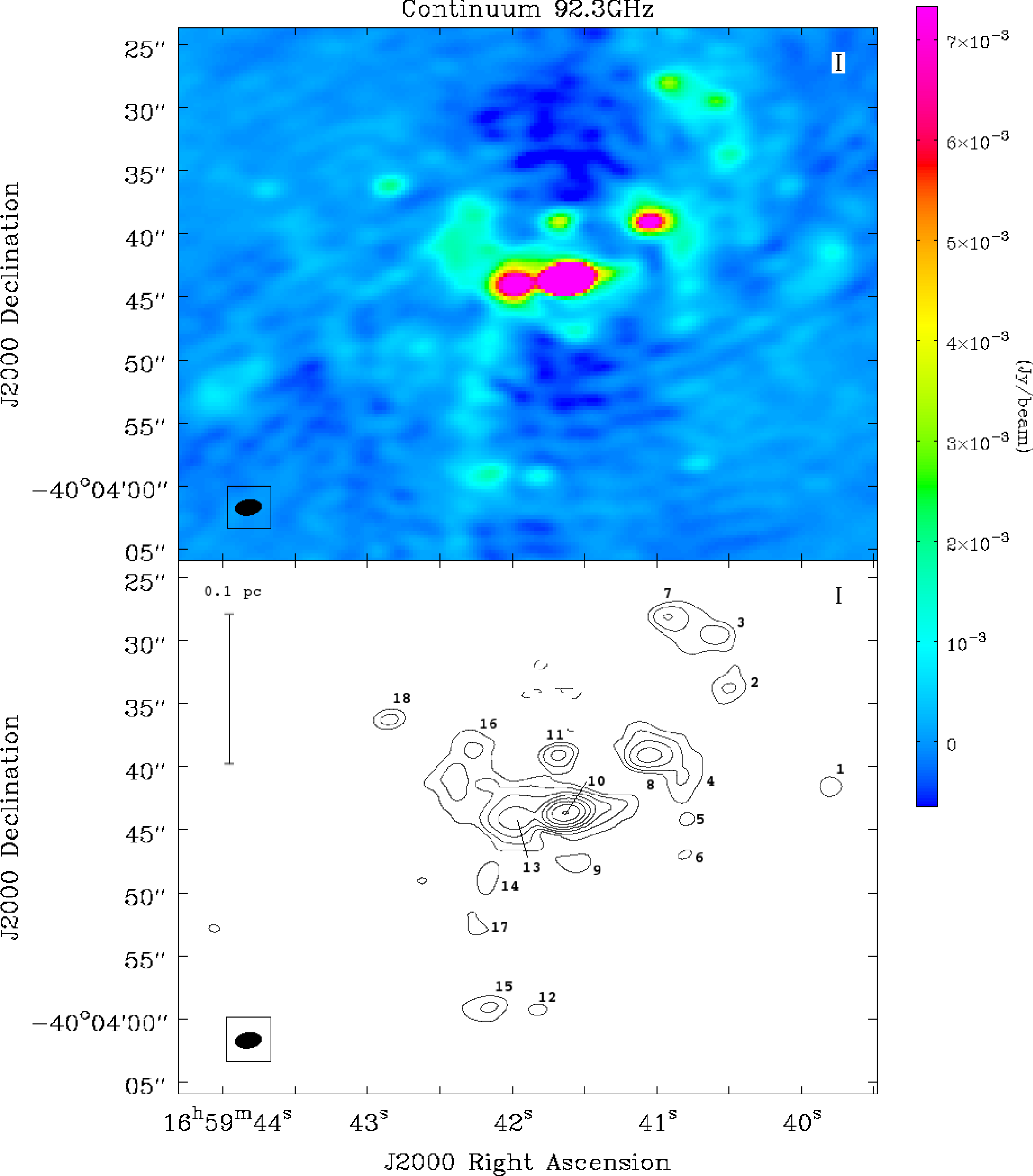
Figure 1: Continuum emission detected at 92.3 GHz toward IRAS 16562$-$3959. Bottom panel: Contours shown correspond to $-15,15,30,60,120,250,500,1000$, and 2000 $\sigma$, with $\sigma=50~{}\mu$Jy beam^-1. $\sigma$ represents the r.m.s. variations of the dynamic range limited image measured at the edge of the field. Compact sources are identified by the number given in Table 2. All sources are within the primary beam.

The continuum sources identified in Figure 1 correspond to compact emission detected above 0.75 mJy in the combined continuum map. This threshold is $\geq 15~{}\sigma$, where $\sigma$ is the r.m.s. variations of the image measured at the edge of the field. This number does not represent random noise, but it arises mainly because of dynamic range limitations of the image. All sources, except perhaps source 18, are embedded in somewhat extended and diffuse emission.

The positions of the continuum sources are given in Table 2. The coordinates correspond to the position of the emission peak determined by using the CASA function maxfit, except for Sources 10 and 13, for which we fit two 2-D Gaussians using the CASA task imfit. For each source, the coordinates determined in the four SpWs are consistent within 0$\farcs$15. Note that the position of Source 10 corresponds to the position of the jet source reported by Guzmán et al. (2010). The deconvolved size of Source 10 is $\lesssim$0$\farcs$4 in each SpW, which is less than one-third of the beam size. Since Source 10 is not completely isolated, we refrain from further analyzing its deconvolved size here.

Table 2 also lists the integrated flux densities in each of the SpWs and the derived in-band spectral index. For Sources 10 and 13, integrated flux densities are derived from the Gaussian fittings. For the rest of the sources, we integrated the flux density within boxes of two times the size of the beam. The uncertainty assumed for each flux density is either $2\sigma\sim 0.1$ mJy or the uncertainty derived from the 2-D Gaussian fit. Best-fit spectral indexes and their uncertainties were obtained by weighted least-squares (or $\chi^{2}$) minimization using the procedure described in Lampton et al. (1976). Unless stated otherwise, this is the procedure we follow throughout this work. The last column of Table 2 shows $\chi^{2}_{r}$, that is, the least-square value divided by the number of degrees of freedom (2).

3.2 HRL emission

HRL emission was detected toward the central Source 10 in three transitions: H40$\alpha$, H42$\alpha$, and H50$\beta$, whose rest frequencies are 99022.95, 85688.39, and 86846.96 MHz, respectively. The spatial distribution of the emission of the three HRLs is similar in all velocity channels and can be described as an unresolved source located within 0$\farcs$1 with respect to the phase center.

Figure 2 shows the spectra of the three HRLs detected toward G345.49+1.47. Table 3 gives the observed parameters of the line profiles at the peak position. From this table and Figure 2 it is evident that the HRL profiles exhibit extended wing emission. Two further characteristics in the observed spectrum are worth mentioning: First, the line located at a velocity of $\sim+125$ km s^-1 in the H40$\alpha$ spectra. This line is narrower than the HRLs, and was identified as one of the SO₂ rotational transitions (see §3.3). Second, an unidentified feature appears in the spectrum of the H40$\alpha$ toward $V_{\rm LSR}<-140$ km s^-1. We have excluded the velocity range affected by this emission in the analysis of the HRLs.

Table 3: Observed parameters of the HRLs

	Peak Flux	$V_{\rm LSR}$ of	FWHM	FWZP	Integrated
	Density	Peak	(km s-1)	(km s-1)	flux
	(mJy)	(km s-1)			(Jy km s-1)
H40$\alpha$	42.6(1)	$-$18.3	44.4	360	2.86(0.05)
H42$\alpha$	32.7(1)	$-$13.6	39.3	227	1.95(0.04)
H50$\beta$	9.1(1)	$-$13.2	50.2	124	0.43(0.03)

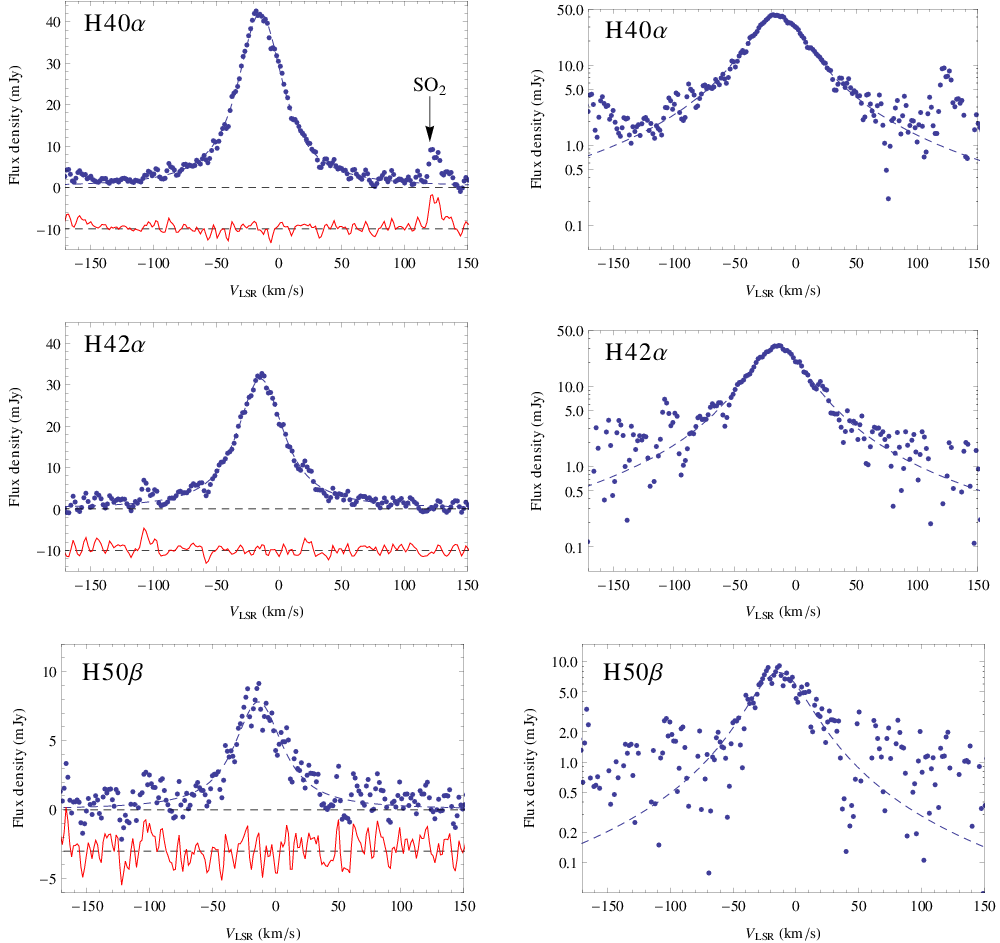
Figure 2: Spectra of the HRLs detected toward G345.49+1.47. Blue dots: Observed data. Dashed lines: Voigt profile fits to the spectra, using the same central velocity and thermal parameter for the three lines. Left column: The flux density plotted in linear scale. The red lines indicate the residuals from the fits. Right column: The flux density displayed in log scale in order to emphasize the wing emission.

3.3 Sulfuretted molecules

Table 4 shows the list of sulfuretted molecules detected in our observations toward G345.49+1.47 and summarizes their main characteristics. The detected species are sulfur monoxide (SO) and its ³⁴S isotopologue, sulfur dioxide (SO₂), carbonyl sulfide (OCS), and carbon monosulfide (CS) and its ³³S isotopologue. We synthesized spatial maps of the emission for all the lines, except of SO₂ $28_{7,21}\rightarrow 29_{6,24}$ (see next section). Columns 2-4 of Table 4 list the frequency, transition, and energy associated with the upper level of the transition in K ($E_{u}=kT$) obtained from the JPL (Pickett et al., 1998) and CDMS (Müller et al., 2001) databases consulted through the Splatalogue (Remijan et al., 2007). Column 5 indicates whether we detect a velocity gradient associated with the central compact component. Column 6 gives the velocity integrated from $V_{\rm LSR}$ $-30$ to 0  km s^-1 line flux within a 5″$\times$5″ box centered on G345.49+1.47 (equatorial orientation). Finally, columns 7-9 display the results of Gaussian fittings to the line flux integrated in the same central 5″$\times$5″ region. The Gaussian parameters roughly describe the most important characteristics of each line, but we stress that Gaussian models to the line profiles are generally poor. Additionally, since the spectral resolution of our data is $\sim$3.0 km s^-1, in the majority of the lines, we have only two independent spectral sampling points per FWHM (column 9 of Table 4). This sampling is too scarce to attempt a detailed modeling of the line profiles.

Table 4: Sulfuretted molecular species detected.

						Gaussian Fitting
Species	Rest Frequency	Transition	$E_{u}/k$	Velocity	Line Flux ($W$)	Peak	$V_{\rm LSR}$	FWHM
	(MHz)		(K)	Gradient	(Jy km s-1)	(Jy)	(km s-1)	(km s-1)
(1)	(2)	(3)	(4)	(5)	(6)	(7)	(8)	(9)
SO	86093.950	$J_{N}=2_{2}\rightarrow 1_{1}$	19.3	Yes	6.22	0.873	$-$12.9	6.6
	99299.870	$J_{N}=3_{2}\rightarrow 2_{1}$	9.2	Yes	14.1	1.777	$-$13.8	7.2
	100029.64	$J_{N}=4_{5}\rightarrow 4_{4}$	38.6	Yes	2.39	0.544	$-$13.2	6.5
34SO	96781.76	$J_{N}=4_{5}\rightarrow 4_{4}$	38.1	Yes	0.099	0.016	$-$13.7	5.4
	97715.317	$J_{N}=3_{2}\rightarrow 2_{1}$	9.1	Yes	1.30	0.196	$-$12.9	6.0
SO2	86639.088	$J_{K_{p}K_{o}}=8_{3,5}\rightarrow 9_{2,8}$	55.2	Yes	0.97	0.118	$-$13.1	7.5
	86828.938	$J_{K_{p}K_{o}}=20_{2,18}\rightarrow 21_{1,21}$	207.8	No	0.025	0.002	$-$10.6	9.4
	97702.334	$J_{K_{p}K_{o}}=7_{3,5}\rightarrow 8_{2,6}$	47.8	Yes	1.32	0.170	$-$12.9	7.3
	98976.294	$J_{K_{p},K_{o}}=28_{7,21}\rightarrow 29_{6,24}$	493.7	No	0.11	0.007	$-$16.8	13.5
	99392.513	$J_{K_{p}K_{o}}=29_{4,26}\rightarrow 28_{5,23}$	440.7	No	0.23	0.023	$-$16.8	9.0
OCS	85139.104	$J=7\rightarrow 6$	16.3	No	1.08	0.130	$-$14.1	6.0
	97301.208	$J=8\rightarrow 7$	21.0	No	1.63	0.251	$-$14.1	5.9
CS	97980.953	$J=2\rightarrow 1$	7.1	No	6.81	1.38	$-$14.2	4.6
C33S	97172.09	$J=2\rightarrow 1$	6.3	No	0.19	0.052	$-$13.5	3.5

The main morphological features of the integrated line maps (or 0th moment) associated with SO, ³⁴SO, and SO₂ (the sulfur oxides) are all similar. Taking SO $J_{N}=4_{5}\rightarrow 4_{4}$ as a representative example, Figure 3 shows contours of the velocity integrated flux within [$-$30.0,0.0] km s^-1. Most of the emission comes from a central bright component with a peak position displaced about 0$\farcs$4 northwest of Source 10. There is also emission from a weaker source located $\sim 4$″ east of Source 10, consistent with the position of Source 13. From Figure 3 we also see that the selected 5″$\times$5″ region encloses well the emission associated with G345.49+1.47, whose parameters for each line are in columns 7-9 of Table 4.

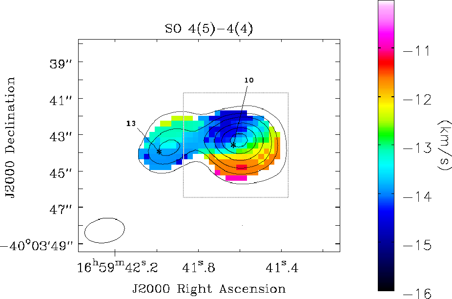
Figure 3: Moment 1 of the SO $J_{N}=4_{5}\rightarrow 4_{4}$ emission detected toward G345.49+1.47 in color scale. Data below 20% of the peak $=0.158$ Jy beam^-1 are masked. Black contours display the emission integrated in the velocity interval between $-22.5$ and $-2.5$ km s^-1. Contours correspond to 10, 20, 30, 50, 70, and 90% of the peak value $=1.16$ Jy beam^-1 km s^-1. The position of the continuum Sources 10 and 13 are indicated by asterisks. The dashed square indicates the 5″$\times$5″integration region used to calculate the line fluxes reported in column 6 of Table 4.

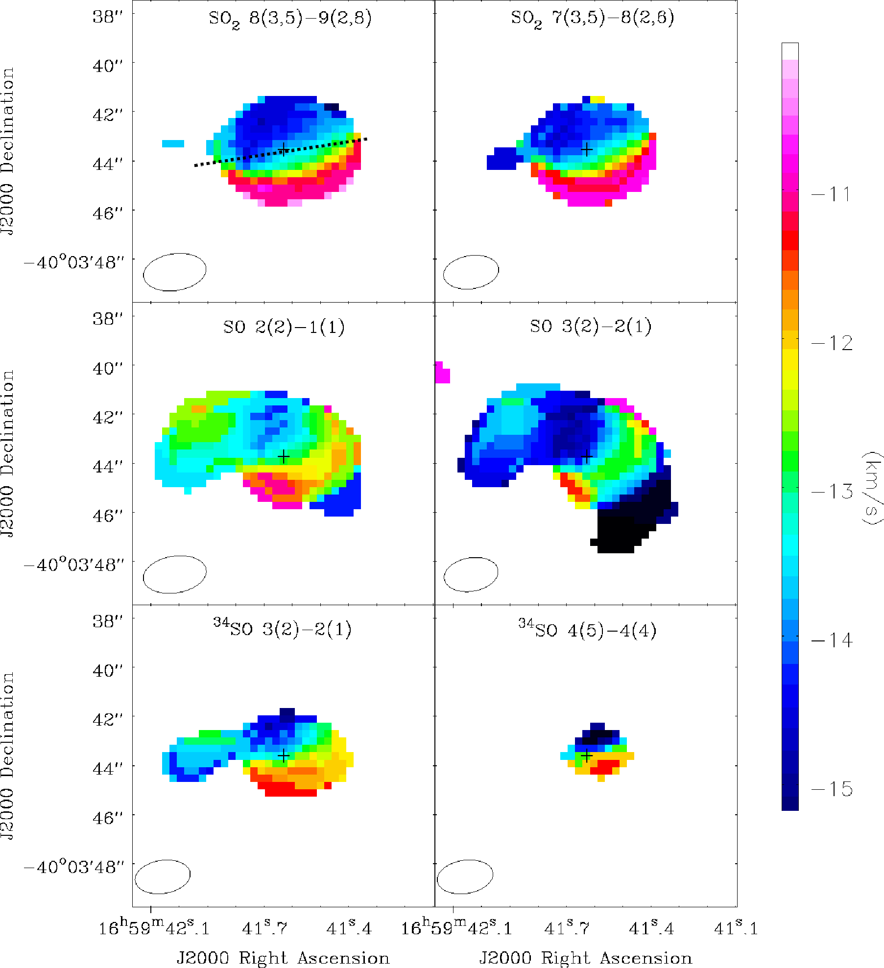
Figure 4: Moment-1 maps of the sulfuretted molecules that display clear velocity gradients associated with G345.49+1.47. The color stretch is equivalent to that of Figure 3. In each panel, a “+” sign indicates the continuum peak. Top left panel: The dashed black line corresponds to the direction inferred for the jet as traced by the ionized lobes (Guzmán et al., 2010).

Figures 3 and 4 show the first moment of some of the sulfur oxide lines. There is a clear velocity gradient associated with G345.49+1.47. The gradient directions and magnitudes are similar in all these transitions.

The morphology of the emission in the other sulfuretted species (CS, C³³S, and OCS) is different than that of the sulfur oxides. Figure 5 shows integrated line maps of the CS 2$\rightarrow$1, C³³S 2$\rightarrow$1, OCS 7$\rightarrow$6, and OCS 8$\rightarrow$7 transitions. The OCS emission is dominated by a single compact source, but displaced from the center of the map by $\sim$0$\farcs$7 to the northwest. The CS and C³³S trace significant extended emission in addition to a compact source near the map center but displaced $\sim 1\farcs 2$ to the northwest. This source is relatively more prominent in the C³³S map with respect to the diffuse extended emission, when compared to CS.

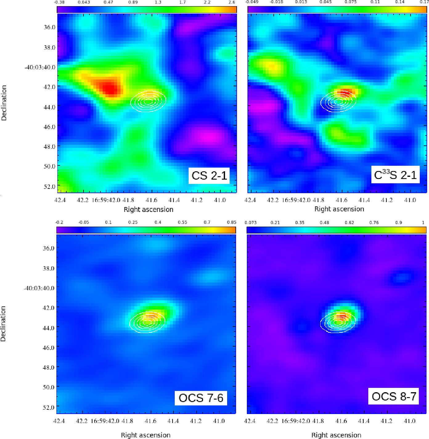
Figure 5: Velocity integrated emission of the CS and OCS lines. The color bars indicate the scale in Jy km s^-1. White contours correspond to continuum emission, dominated by Source 10, at 20, 40, 60, 80, and 90% of the peak (${\rm peak}=0.106$ Jy beam^-1).

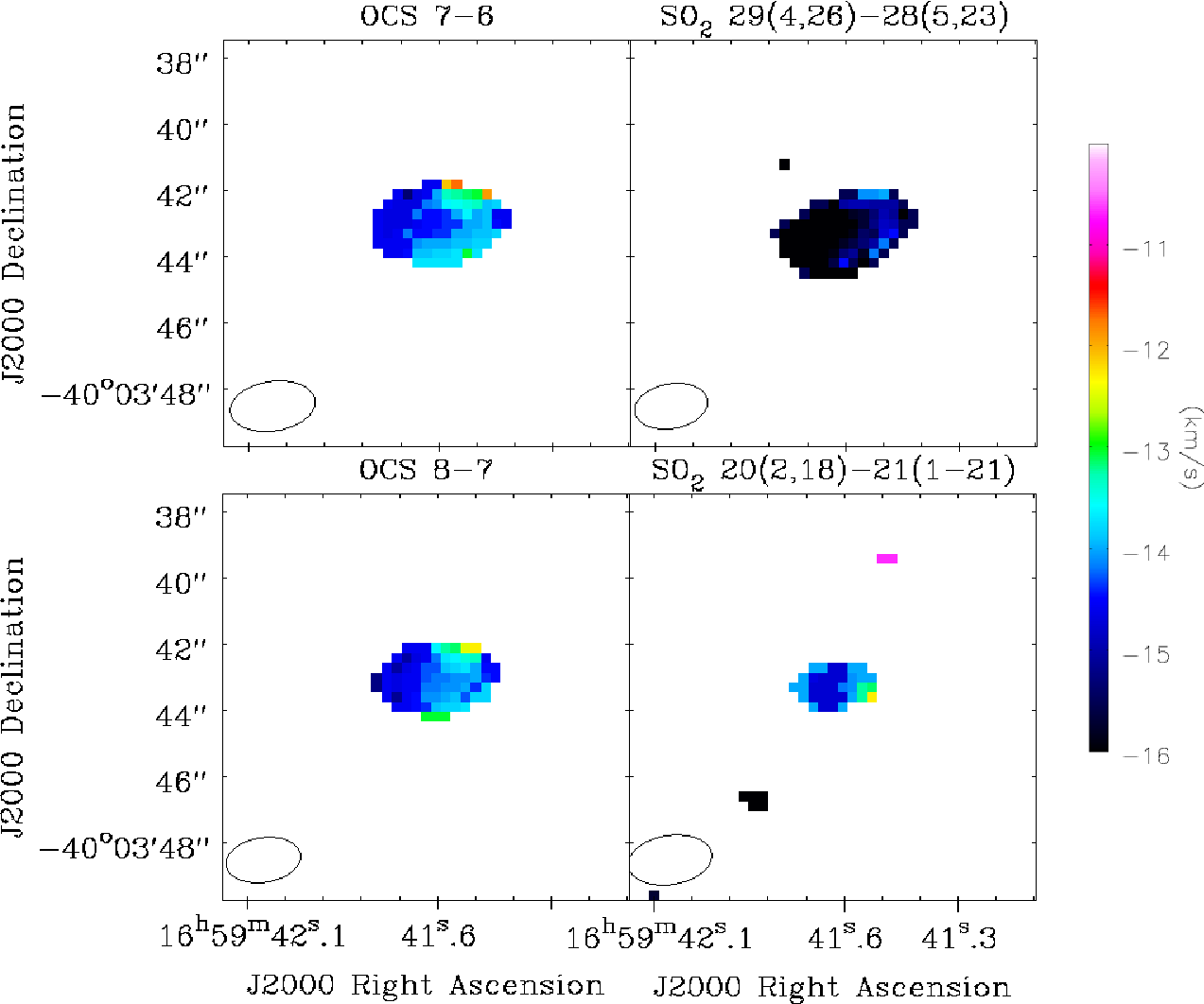
Figure 6: Moment 1 of the sulfuretted molecular line emission associated with G345.49+1.47 that shows no velocity gradient (except for SO₂ $28_{7,21}\rightarrow 29_{6,24}$).

Figure 6 shows first moment maps of the OCS lines and of the SO₂ $20_{2,18}\rightarrow 21_{1,21}$ and $29_{4,26}\rightarrow 28_{5,23}$ transitions. We do not detect any velocity gradient in these lines. Neither CS nor C³³S lines display velocity gradients analogous to the ones traced by the sulfur oxides. Finally, we identify emission from the SO₂ $28_{7,21}\rightarrow 29_{6,24}$ line near the H40$\alpha$ HRL. We expect this SO₂ line to have an apparent velocity displacement of $+126$ km s^-1 with respect to the H40$\alpha$ line, consistent with the observations (see previous section and Figure 2). Having observed other strong SO₂ transitions strengthens this identification.

4 DISCUSSION

In this section, we discuss and analyze the continuum, HRL, and sulfuretted molecular line emission detected toward the compact source G345.49+1.47 and the clump IRAS 16562$-$3959.

4.1 Continuum sources toward IRAS 16562$-$3959

We distinguish three groups of continuum sources associated with the IRAS 16562$-$3959 clump, classified according to their spectral indexes given in Table 2. The indices allow us to propose three plausible mechanisms for the emission.

1. Sources with spectral index $\sim 1$ (Sources 6, 10, and 18): These indexes are characteristic of ionized thermal jets and hypercompact H ii regions (HCH ii regions Guzmán et al., 2012; Keto et al., 2008) and indicate partially optically thick free-free emission. Source 10 is coincident with the jet detected by Guzmán et al. (2010), which is the main interest of the present work and which we analyze in detail in the next sections. The position of Source 18 coincides with the mid-IR source GLIMPSE G345.4977+01.4668 (Benjamin et al., 2003) . An exploration of YSO models with mid-IR fluxes consistent with Source 18, made using the online fitter tool described in Robitaille et al. (2007), indicates that this source is likely an intermediate-mass young star with a luminosity of $\sim 10^{4}\mbox{$\,L_{\sun}$}$. The association with an OH maser (Caswell, 1998) supports this interpretation. The 92 GHz emission from Source 18 most likely arises from a photo-ionized HCH ii region or a stellar wind. This is also possibly the case for Source 6, although it is one of the faintest sources detected in the field.

2. Sources with flat spectrum (Source 1): This spectrum is characteristic of optically thin free-free emission. In Source 1, the excitation arises most likely from shocks, since it is associated with one of the ionized lobes of G345.49+1.47 (see Figure 7).

3. Sources with spectral indices $>2$. Fourteen of the eighteen sources are in this category. They have a mean spectral index of 3.2. For the case of isothermal free-free emission, the spectral index must remain between $-0.1$ and 2 for all density distributions (Rodriguez et al., 1993). However, if the ionized medium has a temperature gradient, then large spectral indices can be obtained (Reynolds, 1986). A more likely explanation is, however, that the spectrum near 100 GHz is substantially affected by optically thin dust (e.g.  Zhang et al., 2007; Beuther et al., 2007; Zapata et al., 2009; Galván-Madrid et al., 2010; Maud et al., 2013). Since the dust emissivity varies as $\nu^{\beta}$, optically thin emission in the Rayleigh-Jeans limit has a spectral index of $\beta+2$. Values of $\beta\sim 1$ can be attributed to grain growth in dense environments (Draine, 2006). However, our spectral indices were derived over a very narrow frequency range of 85-100 GHz. Hence, since we cannot separate the free-free component from the dust component, we do not draw any definite conclusions about the nature of the dust grains. We propose that all these sources are associated with dust emission arising from molecular cores within the young stellar population of IRAS 16562$-$3959. Among these, we highlight Sources 12 and 13. Source 12 position is consistent with IR sources GLIMPSE G345.4906+01.4655 and 2MASS 16594180-4003591 (Skrutskie et al., 2006), and the results of the YSO online fitting tool indicate that it corresponds to a source with a bolometric luminosity of $\sim 1000\mbox{$\,L_{\sun}$}$. Source 13 is the second most luminous source detected toward the IRAS 16562$-$3959 field, and its position suggests that it may harbor the powering source of the North-South bipolar molecular outflow detected by Guzmán et al. (2011). Finally, we note that Sources 9 and 14 seem to be associated with mid-IR point sources detected by IRAC at 4.5 µm (Fazio et al., 2004; Benjamin et al., 2003).

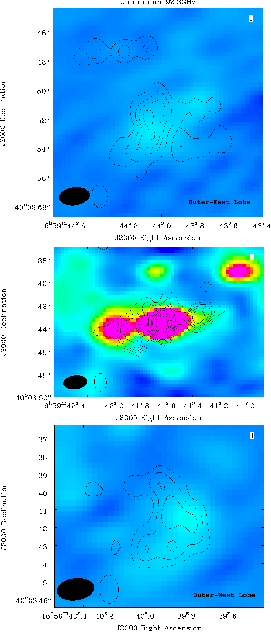
Figure 7: Comparison between the 92 GHz continuum (color background image) and 8.6 GHz emission (black contours) reported by Guzmán et al. (2010) following their naming convention. In the bottom left corner of each panel, we show the synthesized beams, filled and outlined for the 92 GHz and 8.6 GHz data, respectively. Top and bottom panel: Emission detected toward the O-E and O-W lobes, respectively. The central panel shows the emission toward the inner lobes flanking the central jet source identified by Guzmán et al. (2010).

4.2 The ionized jet observed at 92 GHz

The three panels of Figure 7 show images of the 92 GHz emission observed toward the jet and the lobe system reported by Guzmán et al. (2010), overlaid with contours at 8.6 GHz emission. In this work, we refer to 92 GHz emission as the emission calculated combining the four SpWs. Following the Guzmán et al. (2010) naming convention, the two outermost lobes are referred to as outer-east (O-E) and outer-west (O-W) lobes, while the two innermost as inner-east (I-E) and inner-west (I-W) lobes.

Source 10 coincides, within the uncertainties, with the jet source. Furthermore, the spectral indexes of the radio continuum from the jet below 10 GHz ($0.85\pm 0.15$) and of the 92 GHz emission of Source 10 ($1.0\pm 0.1$) are similar. We conclude that Source 10 is the 92 GHz counterpart of the ionized jet and that the emission at both frequency ranges comes from partially optically thick ionized gas.

Figure 8 presents the radio continuum spectra of the ionized jet in the range from 1 to 100 GHz. This spectra is well fitted by a power law in frequency with an spectral index of $0.92\pm 0.01$ over the entire frequency range, consistent with partially optically thick thermal free-free emission (Anglada, 1996; Villuendas et al., 1996; Jaffe & Martín-Pintado, 1999). While this is the dominating emission mechanism, it is likely that at the highest frequencies a small fraction of the emission arises from thermal dust. We note that the ALMA spectrum of Source 10 is marginally steeper than the one measured at centimeter wavelengths alone, which might be attributed to dust emission. By fitting the data with two power laws, one for partially optically thick free-free emission and the other with an spectral index equal to 3, representing the dust contribution, we find that the flux attributable to dust is $\sim 11$ mJy at 92 GHz, that is, $\sim$10% of the total flux coming from G345.49+1.47.

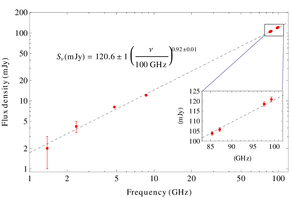
Figure 8: Radio continuum flux density vs. frequency (log-log plot) for G345.49+1.47. The dashed line indicates a least-squares power law fit over the whole frequency range, giving an spectral index of $0.92$. The fit parameters of the spectrum are shown in the figure. The inset displays a zoom over the range of data from ALMA. ATCA data shown for frequencies below 10 GHz are taken from Guzmán et al. (2010).

The ionizing photon flux needed to maintain the recombination equilibrium is $\geq 5.8\times 10^{46}$ s^-1 (Guzmán et al., 2012), which is larger than the typical ionizing fluxes needed to maintain the typical mJy-level flux of jets detected in centimeter bands. The momentum rate estimated for G345.49+1.47, of $\sim 10^{-3}$ $\,M_{\sun}$ yr^-1 km s^-1(Guzmán et al., 2010), is approximately two orders of magnitude smaller than the minimum required for the jet in order to shock-ionize itself (Johnston et al., 2013; Curiel et al., 1989). Furthermore, as analyzed in the subsequent sections, the value of the momentum rate computed for G345.49+1.47 is likely overestimated since the velocity of the ionized gas is $<300$ km s^-1. We conclude that the ionizing UV photons come from the young high-mass star itself, from which we expect fluxes larger than $10^{47}$ s^-1 (see, for example Martins et al., 2005). This is despite the evidence that G345.49+1.47 appears to be accreting at a high rate, which in theory should quench the development of an H ii region (Walmsley, 1995) or decrease substantially the effective temperature of the young star (Hoare & Franco, 2007; Hosokawa & Omukai, 2009).

We also detected emission at the positions of the outer lobes of the jet, as shown in Figure 7. Source 1 of Table 2 corresponds to the O-W lobe. This source has a flat spectrum, characteristic of optically thin free-free emission, which is expected since the emission from the ionized lobes is already optically thin at centimeter wavelengths. The O-E lobe is associated with diffuse emission above $5\sigma$, shown in Figure 7. This identification gives confidence that most features shown in the color map of Figure 7 are real. The flux density of the outer lobes at 92 GHz, corrected for primary beam response and integrated over the regions shown in Figure 7, are 4.5 and 5.8 mJy for the O-W and O-E lobes, respectively. These fluxes are consistent with the ones reported by Guzmán et al. (2010), scaled with frequency as $\nu^{-0.1}$.

Emission from the inner lobes is, however, difficult to disentangle from our data. This is partly because the angular resolution of the ALMA data is approximately two times lower than that of the centimeter wavelength observations, producing an overlap of the emission from the inner lobes with that of nearby sources and from the jet. We expect the inner lobes to have $\sim 4$ mJy each. Source 13, as remarked previously, displays a dustlike emission spectrum, and it is not a free-free counterpart of the inner-east lobe.

4.3 Broadening of the HRLs associated with the jet G345.49+1.47

Theoretical work predicts that, in addition to thermal and turbulent broadening, HRLs should be broadened by the linear Stark effect, namely, the splitting and displacement of the atomic energy levels by an electric field. For interstellar ionized regions and for HRLs in the radio and millimeter regions of the spectrum, the most important mechanism for Stark broadening is scattering with electrons under conditions where the impact approximation is valid (Griem, 1967). The Stark broadening redistributes the energy in the line over a frequency interval larger than that produced by the thermal and turbulent broadening. The predicted line shape is a Voigt profile, which corresponds to the convolution of a Gaussian component, produced by the thermal and turbulent motions of the recombining atoms, and a Lorentzian component, produced by the impacts with electrons. Toward the center of the line, the profile is nearly Gaussian, whereas toward the wings, it is nearly Lorentzian.

The theory of hydrogen Stark broadening was developed after a few setbacks (see Gordon & Sorochenko, 2002, for a historical account) in which astronomical observations played a crucial role. Recently, the theory was again questioned by observations (Bell et al., 2000), triggering a debate settled recently by Alexander & Gulyaev (2012). Direct detection of clear-cut Voigt profiles is an important confirmation of the currently accepted broadening theory, and until now, these profiles have not been unambiguously observed in the astronomical context.

Most of the reported HRL observations in the literature are not sensitive enough to detect the wing emission from the Voigt profiles, and consequently, their profiles appear roughly Gaussian. The presence of Stark broadening is inferred indirectly, usually from observations of two HRLs with different principal quantum numbers. Because the pressure broadening increases with the transition quantum number as $n^{7.5}$, the thermal broadening is determined from the width of the HRL with the smaller $n$ (higher frequency), and the pressure broadening is estimated from the increase of the line width of the high $n$ transition with respect to that of the low $n$, assuming optically thin conditions (Keto et al., 2008; Sewiło et al., 2011; Galván-Madrid et al., 2012). In the few cases where there is a direct wing detection, it is weak (e.g., Simpson, 1973; Smirnov et al., 1984; Foster et al., 2007; von Procházka et al., 2010). Apparently, the clearest previous case of pressure broadening is shown in carbon recombination lines observed in absorption towards SNR Cas A (see Stepkin et al., 2007, and references therein). The lack of direct detection of the wing emission in Voigt profiles from HRLs is likely due both to their intrinsic low intensities and to the wide velocity range they span, requiring for identification sensitive observations and flat or linear instrumental baselines that just have become available with the new generation of radio telescopes.

4.3.1 Voigt profile fitting

Figure 6 shows the HRL profiles at the peak position. They display evident wing emission, which we fit using Voigt functions. Figure 2 also shows the results of Voigt profile fits and residuals. The Voigt function is characterized by four parameters: the value at the peak, the central velocity, and the Lorentzian and Gaussian widths. We parameterize the Gaussian width ($\Delta_{G}$) using the relation $\Delta_{G}=0.22\sqrt{T\,\text{(K)}}$ km s^-1 (Gordon & Sorochenko, 2002, § 2.2.2), where $T$ is the temperature of the gas that emits the HRL.

Best-fit parameters are obtained by minimization of the weighted-squared difference

$$\sum_{\rm HRLs}\sum_{V_{l}<v_{i}<V_{m}}\left(\frac{{\rm HRL}({v_{i}})-\mathcal{V}({\rm Peak},V_{0},\delta_{L},T;v_{i})}{\sigma}\right)^{2}~{}~{},$$ (1)

where $\sigma=1$ mJy is the noise per channel, the first sum runs over the three recombination line data (${\rm HRL}=$H40$\alpha$, H42$\alpha$, H50$\beta$), and the second sum runs over the channels ($v_{i}$) between the $V_{\rm LSR}$ limits $V_{l}=-80$ and $V_{m}=100$ km s^-1. These velocity limits exclude the regions where we expect contamination from He or C recombination lines, or molecular lines. The expression $\mathcal{V}({\rm Peak},V_{0},\delta_{L},T;v_{i})$ represents the value of the Voigt function associated with its four parameters (${\rm Peak},V_{0},\delta_{L}$ and $T$), evaluated at velocity $v_{i}$. The Voigt function parameters are allowed to be different between the HRLs, except for $T$. Our best-fit model indicates that this temperature is $T=2000^{+6000}_{-1000}$ K. The 1-$\sigma$ uncertainty range of best-fit temperatures is large since the thermal Gaussian width is much narrower than the wings. However, the range of values is within what is expected for ionized regions in the Galaxy. In particular, we do not find evidence of nonthermal Gaussian broadening, as may be expected from turbulence. In the following analysis, we fixed the value of the temperature of the ionized gas as $T=7000$ K, which is close to the expected electronic temperature for the galactocentric distance of G345.49+1.47 (6400 K, Paladini et al., 2004) and within the uncertainty.

Table 5 lists the best-fit values and uncertainties of the Voigt-function fittings to the three HRLs detected, assuming $T=7000$ K. The central velocity of the three lines is the same within the errors. The half-width at half-maximum of the Lorentzian portion of the profiles, $\delta_{L}$, is between 18 and 20 km s^-1. The Voigt function model, with and without constrained temperature, performs better than single or double Gaussian models evaluated by a heuristic visual assessment and according to the quantitative Akaike information criterion (AIC, Feigelson & Babu, 2012, § 3.7.3). The AIC penalizes the weighted least-squared difference by adding two times the number of free parameters of the specific model. The free parameters of the Voigt model are 10, while for two independent Gaussians per HRL they are 18. The correlation between adjacent channels introduced by the Hanning smoothing of the data does not affect the validity of the application of the AIC.

Table 5: Voigt fitting parameters of the HRLs

	Peak Flux	$V_{0}$	${\delta_{L}}$	Characteristic
	Density	(LSR)	(km s-1)	Density
	(mJy)	(km s-1)		($10^{7}\,$cm-3)
H40$\alpha$	$41.4\pm 0.8$	$-14.8\pm 0.5$	$18.6\pm 1.0$	$9.7\pm 0.5$
H42$\alpha$	$30.1\pm 0.8$	$-14.8\pm 0.7$	$19.2\pm 1.0$	$6.9\pm 0.4$
H50$\beta$	$7.7\pm 0.8$	$-13.3\pm 3.0$	$20.2\pm 4.0$	$3.8\pm 0.8$

Note. — Assuming $T_{e}=7000$ K for the three lines.

4.3.2 Electron density

The electron density can be derived theoretically from Voigt fitting of the HRLs using the relation between $\delta_{L}$ and the physical parameters of the ionized gas, first computed by Griem (1967). For the range of principal quantum numbers appropriate for this work, this relation can be written to an adequate accuracy level as (Walmsley, 1990)

$$\delta_{L}=2.72~{}{\rm km~{}s^{-1}}\left(\frac{n}{42}\right)^{7.5}{\Delta n}^{-1}\left(\frac{N_{e}}{10^{7}~{}{\rm cm^{-3}}}\right)\left(\frac{T_{e}}{\rm 10^{4}~{}K}\right)^{-0.1}~{}.$$ (2)

In Equation (2), the HRL is produced by the decay of an electron from the $(n+\Delta n)$ to the $n$ quantum level. $T_{e}$ is the electron temperature, and $N_{e}$ is the free electron density. The last column of Table 5 gives the electron densities derived from the observed values of $\delta_{L}$. We find a characteristic value for the electron density of $5\times 10^{7}$ cm^-3.

4.4 Ionized wind model: continuum and recombination lines

In this section, we present a simple model of the jet that explains simultaneously the main characteristics of the continuum and HRL emission.

4.4.1 Collimated ionized jet model and continuum spectrum

A useful parameterization of the jet structure is given in Reynolds (1986). This parameterization is flexible enough to reproduce the continuum emission spectrum for most ionized jetlike sources, including G345.49+1.47 (Guzmán et al., 2010). We use the same notation as Reynolds (1986), with a few differences that are made explicit below. Figure 9 depicts the geometry of the jet model. Quantities with a 0-subscript ($r_{0},w_{0}$, etc.…) correspond to those at a fixed fiducial radius $r_{0}$, rather than at the inner termination radius of the jet, as used in Reynolds (1986). We choose as the fiducial radius $r_{0}=100$ AU. For parameters at the the inner termination radius, we use an i-subscript ($r_{\rm i},w_{\rm i}$, etc.…), and for quantities at the outer limit of the jet, an f-subscript.

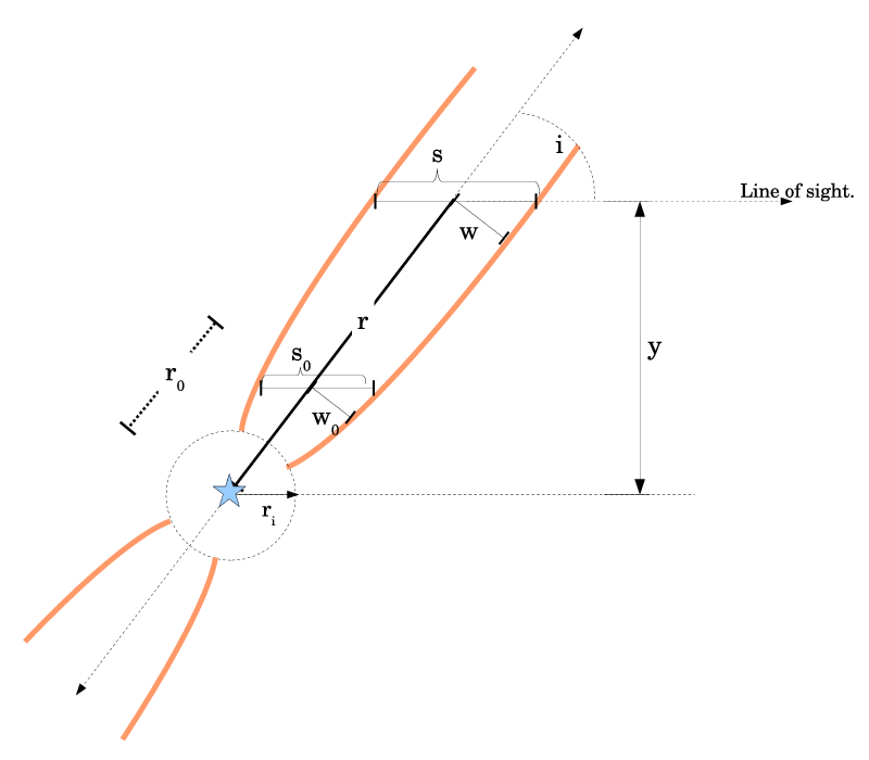
Figure 9: Geometrical model of the jet plus a symmetrical counterjet. This figure is based on Figure 1 from Reynolds (1986). It represents a cut of the jet+counterjet system in the plane that includes the axis of the jet and the line of sight. The jet+counterjet system is assumed to be axisymmetric.

We use the following relations

$$w(r) =w_{0}\left(\frac{r}{r_{0}}\right)^{\epsilon}$$ aperture power law, (3)

$$y(r) =r\sin(i)$$ projected distance, (4)

$$\theta_{0} =\frac{2w_{0}}{r_{0}}$$ collimation factor, (5)

$$s(r) =\frac{2w(r)}{\sin(i)}$$ path length. (6)

The shape of the jet is given by $\epsilon$ and $\theta_{0}$, with $0.5<\epsilon\leq 1$. A conical wind corresponds to $\epsilon=1$. The physical size of the jet is given by $w_{0}$, $r_{\rm i}$, and $r_{\rm f}$. We assume that the ionized gas consists only of hydrogen, with a constant ionization fraction. Therefore, the density (in cm^-3) of the ionized gas is equal to two times the free electron density $N_{e}(r)$. The density $N_{e}(r)$, velocity $v(r)$, and temperature $T(r)$ are assumed to depend as power laws with the distance from the origin as

$$N_{e}(r) =N_{e,0}(r/r_{0})^{q_{n}}~{}~{},$$ (7)

$$v(r) =v_{0}(r/r_{0})^{q_{v}}~{}~{},$$ (8)

$$T(r) =T_{0}(r/r_{0})^{q_{T}}~{}~{}.$$ (9)

If we assume that the velocity of the ionized gas is in the axis direction and away from the origin, $q_{v}>0$ and $q_{v}<0$ represent, respectively, accelerating and decelerating winds. Considering a constant ionization fraction, mass conservation implies that $q_{n}=-q_{v}-2\epsilon$. We assume that the free-free absorption coefficient ($\kappa_{\nu}$) has a power law dependence with temperature ($\propto T^{-1.35}$) and density ($\propto N_{e}^{2}$, see, for example, Wilson et al., 2009, §10.6). This assumption implies that the free-free optical depth associated with a line of sight that intersects the jet axis, given approximately by $\tau(\nu,r)\approx\kappa_{\nu}(r)\times s(r)$, also behaves as a power law on $r$ given by

$$\tau(\nu,r) =\tau(\nu,0)(r/r_{0})^{q_{\tau}}~{}~{},$$ (10)

$$\text{with}\ q_{\tau} =\epsilon+2q_{n}-1.35q_{T}~{}~{}.$$ (11)

The flux density predicted from the jet model presented here is derived in appendix A. In the intermediate range of frequencies where the jet is neither completely optically thin nor thick, the flux density is given by

$$S_{\nu} =S_{\nu_{0}}\left(\frac{\nu}{\nu_{0}}\right)^{\alpha_{\rm op}}~{}~{},$$ (12)

$$\alpha_{\rm op} =2+2.1(1+\epsilon+q_{T})/q_{\tau}~{}~{},$$ (13)

where $S_{\nu_{0}}$ is the flux at the fiducial frequency $\nu_{0}$. Equation (12) is a rising power law in frequency, as observed in G345.49+1.47 over almost two decades in frequency (see § 4.2) and toward several other jets and broad-HRL HCH ii regions (see Guzmán et al., 2012; Jaffe & Martín-Pintado, 1999, and references therein).

The most important caveat associated with the model is that the data constraints on the parameters are not tight. The selection of particular parameters is heuristic and starts with what is considered the simplest choice. In our case, we will explore isothermal models ($q_{T}=0$) with a constant ionization fraction. These constraints are not sufficient to determine uniquely the jet parameters. There are still five free parameters: the inclination angle ($i$), the fiducial aperture ($\theta_{0}$), the density at the fiducial radius ($N_{e,0}$), and two exponents: the shape exponent ($\epsilon$) and the density exponent ($q_{n}$). The constraints imposed by the spectral energy distribution, given in Equation (12), are only two: $S_{\nu_{0}}$ and $\alpha_{\rm op}$. The inclination angle $i$ was estimated as $\sim 45$° by Guzmán et al. (2010), based on the appearance of the 2 µm image of the inner cavity, and we use this value throughout.

With these constraints, we find that the observed continuum spectrum of G345.49+1.47 is well modeled as free-free emission arising from a fully ionized, isothermal (7000 K), conical ($\epsilon=1$) wind, with a collimation factor $\theta_{0}=0.33$. There are still two degrees of freedom on the model, and this particular selection of $\epsilon$ and $\theta_{0}$ is arbitrary.

4.4.2 Model prediction for HRLs

In this section, we discuss the HRLs expected from the model presented in the previous section. The goal is to test whether we can reproduce the observed line fluxes and profiles using only Stark and thermal Gaussian broadening. This would imply, at least as far our observations can constrain, that the observed line wings are not due to bulk motions of the ionized gas. Even though the lines seem to be well reproduced by Voigt profiles, there is a problem with the interpretation of the pressure broadening: the observed ratio between the line widths of the $\alpha$ and $\beta$ transitions is not as expected from Equation (2), using a single characteristic density. Equation (2) predicts that the FWHMs should be in the ratio $\sim(50/40)^{7.5}/2\approx 2.7$, while the observed value is $\sim 1$. We will come back to this issue at the end of the section.

The line flux expected from the jet model described in the previous section, $S_{\rm\nu,L}$, under assumptions of isothermality and local thermodynamic equilibrium (LTE), is derived in appendix B. $S_{\rm\nu,L}$ is given by

$$S_{\rm\nu_{0}}\left(\frac{\nu}{\nu_{0}}\right)^{\alpha_{op}}\left(\Gamma\left(\frac{\alpha_{\rm op}-2}{2.1}\right)^{-1}\int_{0}^{\infty}\tau^{\frac{\alpha_{\rm op}-4.1}{2.1}}\left(1-e^{-\tau(1+\Delta\nu_{\rm L}\phi(\nu,N_{e}))}\right)d\tau-1\right)~{},$$ (14)

where $\phi(\nu,N_{e})$ is the line profile ($\int\phi d\nu=1$), and $\Delta\nu_{L}$ (defined in appendix B) depends only on the specific transition and on the gas temperature. For the three lines considered in this work, $\Delta\nu_{L}$ takes the value

$$\{\Delta\nu_{\rm H40\alpha},\Delta\nu_{\rm H42\alpha},\Delta\nu_{\rm H50\beta}\}=\{10.8,~{}7.9,~{}3.0\}~{}{\rm MHz}\times\left(\frac{T_{e}}{10,000{\rm K}}\right)^{-1.25}~{}~{},$$ (15)

where the temperature dependence form is appropriate for frequencies around 100 GHz (Lang, 1999). The line profile $\phi(\nu,N_{e})$ is a Voigt function with density parameter $N_{e}$. This density is not constant but depends on the integration variable (the continuum opacity $\tau$) as $N_{e}(\tau)=N_{e,0}(\tau/\tau_{0})^{q_{n}/q_{\tau}}$. This relation can be deduced from Equations (7) and (10).

We test the hypothesis that the observed line wings are reproducible with negligible bulk motions. We assume in Equation (15) that the line profiles have the same central frequency instead of being displaced by their corresponding Doppler shifts and that the gas velocity behaves as $v_{0}(r/r_{0})^{q_{v}}$ (Equation 8). Our hypothesis of negligible bulk motions is equivalent to $v_{0}$ being small compared to the line widths.

Figure 10 shows with a continuous red line the expected profiles derived from Equation (14) using $S_{\nu_{0}}=S_{\rm 100\,GHz}=120.6$ mJy, $\alpha_{op}=0.92$, and $T_{0}=7000$ K. Either of the following jet parameters give indistinguishable predictions

$$\begin{split}\epsilon=1&,~{}~{}\theta_{0}=0.33,~{}~{}N_{e,0}=2.19\times 10^{7}~{}\text{cm}^{-3}\quad\text{(conical wind),}\\ \epsilon=0.5&,~{}~{}\theta_{0}=0.23,~{}~{}N_{e,0}=2.82\times 10^{7}~{}\text{cm}^{-3}~{}~{}.\end{split}$$ (16)

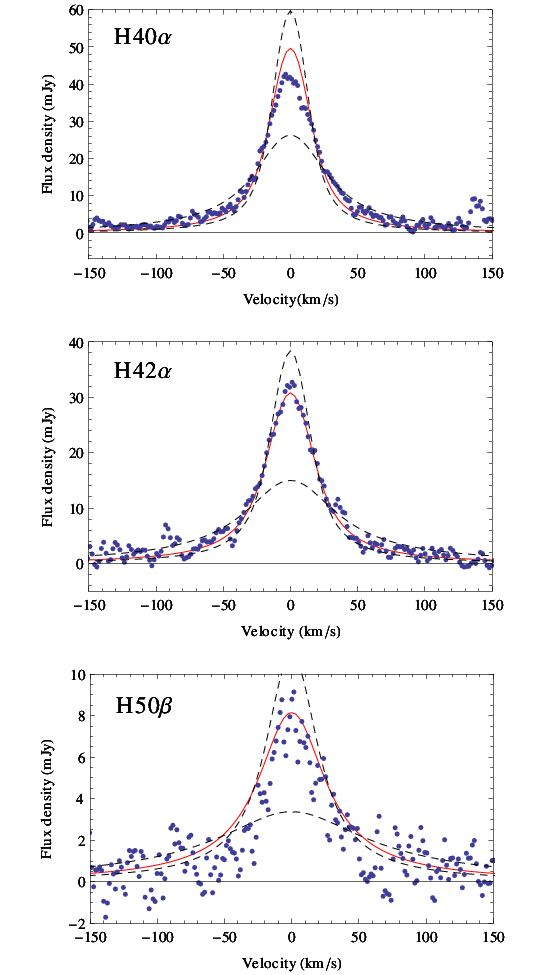
Figure 10: Blue dots: Spectra of the observed HRLs toward G345.49+1.47. Continuous red line: Prediction of the emission arising from a jet model with negligible velocities and the parameters given in Equation (16). The velocity scale is shifted to the common central velocity of the HRLs of $-14.8$ km s^-1. Dashed lines: Model predictions of the HRLs using a smaller and larger fiducial aperture compared with the optimal value, predicting, respectively, the flatter and sharper curves.

For each value of the geometrical aperture exponent $\epsilon$, there is an optimal fiducial aperture $\theta_{0}$ that predicts approximately the same HRLs. Therefore, the HRL observations have decreased the degeneracy degree from 2 (see previous section) to 1. The optimal $\epsilon$-$\theta_{0}$ curve has as extreme points the conical ($\epsilon=1$) and $\epsilon=0.5$ aperture laws given in Equations (16). The dashed lines in Figure 10 show the behavior of the model predictions for $\theta_{0}$ larger and smaller than the best-fit aperture angle ($\theta_{0,{\rm opt}}$). If $\theta_{0}>\theta_{0,{\rm opt}}$, a larger fraction of the gas is more diffuse, increasing the peak-to-width ratio appearance of the line. This is illustrated in Figure 10 with the narrower and sharp dashed curve, representing the prediction for a conical wind and $\theta_{0}=0.4$. On the other hand, if $\theta_{0}<\theta_{0,{\rm opt}}$, more emission arises from more dense gas, and the HRLs widen, illustrated by the flatter curve ($\theta_{0}=0.2$).

We find that the predicted flux level and shape of the lines are consistent with the data, which is remarkable considering the simplicity of the model, namely, no bulk motions and LTE assumptions. Quantitatively, LTE can be justified since the typical densities derived for G345.49+1.47 ($\sim 5\times 10^{7}$ cm^-3, see Table 5) are $\sim 1$ order of magnitude larger than the critical electron density given by Equation (3.1.6) from Strelnitski et al. (1996). These higher electronic densities increase the collision rates and damp non-LTE effects.

The model also reproduces the relation observed between the line widths of the $\alpha$ and $\beta$ transitions, which are not in the ratio of $2.7$ as would be expected from Equation (2). Usually in the literature, a strong dependence of line width with quantum number is a common criterion to identify pressure broadening in HRLs from young massive stars (e.g., see Lumsden et al. 2012, using IR HRLs; and Keto et al. 2008). The reason for the unusual behavior of the G345.49+1.47 lines is that $\alpha$ transitions, in contrast to $\beta$ transitions, are associated with large line opacities that saturate the line near the peak, increasing the line width. The flux-weighted line peak optical depth for the H50$\beta$ line is $\sim 1$, while for the $\alpha$ lines, it is $>6$. Accordingly, we stress that the values deduced for the density from independent Voigt profiles fittings, given in Table 5, represent average values that need to be interpreted with care.

The agreement between the model and the data is not perfect, showing discrepancies near the line center of H40$\alpha$ and in the width of the H50$\beta$ line. Typically, the analysis of hydrogen recombination lines in the millimeter and sub-millimeter wavelengths includes large corrections due to non-LTE effects (Mezger & Palmer, 1968; Peters et al., 2012; Báez-Rubio et al., 2013). We might be observing these effects near the line center where we expect the largest opacities. Finally, we note that despite the model reproduces a lower ratio between the widths of the $\beta$ and $\alpha$ transitions compared to that associated with optically thin LTE conditions, the data seems to accent this feature even more.

4.5 Sulfuretted molecular emission from G345.49+1.47

Sulfuretted molecules, and specially sulfur oxides, seem to increase their abundance $\sim$3-4 orders of magnitude in high-mass star formation regions when evolving from IR luminous massive cores (Herpin et al., 2009) to a hot core phase (van der Tak et al., 2003; Jiménez-Serra et al., 2012). These molecules, particularly SO₂, have become common tracers of rotation in disklike structures associated with HMYSOs (see Fernández-López et al. 2011 and references therein; also Jiménez-Serra et al. 2012). Figures 3 and 4 show that this also seems to be the case for G345.49+1.47.

The analysis presented in the following sections has made extensive use of the Splatalogue, JPL, CDMS and Basecol (Dubernet et al., 2013) catalogs and databases to obtain transition frequencies, energies, partition functions, Einstein coefficients, and collision rate coefficients.

4.5.1 Qualitative chemical analysis of the sulfuretted molecules emission distribution

All sulfuretted molecules in Table 4 display compact emission associated with the central source G345.49+1.47. While the sulfur oxides emission coincides with the jet location and several of their transitions show characteristic disklike velocity gradients, the OCS and especially the CS and C³³S lines peak away from the jet and do not exhibit velocity gradients. The morphological similarity of the CS and C³³S maps suggests that, at least for CS, self-absorption is not the main cause of the observed displacement. Based on Earth sulfur isotopic ratios $[\,^{32}{\rm S}:\,^{34}{\rm S}:\,^{33}{\rm S}]=[126.7:5.6:1.0]$ given by De Biévre & Taylor (1993), we expect an opacity of the C³³S line $\sim 130$ times smaller than that of the main isotopologue.

In the rest of this section, we address the following questions: i) What determines which transitions trace the velocity gradient that we attribute to a disklike structure? ii) Why do sulfur oxides seem to be intimately associated with the G345.49+1.47 jet free-free continuum? ii) Why do the OCS and CS lines peak away from the jet location?

To answer the first question, we note that two groups of lines do not show the disklike velocity gradient: the SO₂ transitions associated with upper energy levels $>200$ K, and the OCS and CS transitions. We attribute the lack of detection of the velocity gradient in the first case to the relatively poor angular resolution of our data. The emission from the high-energy SO₂ lines most likely arises from the hot inner regions of the disklike structure, located close to the central young star (or stars). If this is the case, we should detect the velocity gradients in these transitions using better angular resolution observations. On the other hand, emission from the CS and C³³S lines arises from a different location compared to the sulfur oxide lines.

The displacement between the OCS and sulfur oxides emission is smaller, but it is highly unlikely the OCS emission is associated with an unresolved hot gas component because, as derived in section 4.5.2, OCS is in a relatively low excitation state ($\sim 40$ K). Subthermal excitation does not play a role, since the density estimation made from dust continuum in Guzmán et al. (2010) ($\gtrsim 10^{5}$ cm^-3) is above the OCS transitions’ critical densities of approximately $3\times 10^{4}$ cm^-3 (Green & Chapman, 1978). Summarizing, we propose that the high-energy SO₂ lines trace an unresolved hot component and hence do not show a velocity gradient, and that OCS and CS arise from the outer gas near the G345.49+1.47 core.

The close match of the SO and SO₂ emission with the central free-free jet emission is consistent with the hot core model of Charnley (1997). According to this model, SO and SO₂ are created in the gas phase on timescales $\sim 10^{3\text{-}4}$ yr, while OCS and CS arise in $\sim 10^{4\text{-}5}$ yr. Therefore, since we expect G345.49+1.47 to be younger than $10^{5}$ yr (Guzmán, 2012), SO, ³⁴SO, and SO₂ have been synthesized in the irradiated disklike structure, but only insignificant amounts of OCS or CS would have been formed. This explains the absence of OCS and CS in the rotating disklike structure, but, why does OCS appear to be associated with the G345.49+1.47 core? Charnley (1997), Hatchell et al. (1998), and van der Tak et al. (2003), all report difficulties in reproducing the observed abundance of OCS from observed hot cores, resorting to grain-mantle chemistry and evaporation from solid-phase ices as additional sources of OCS. SO₂ and OCS have been detected in interstellar ices (Gibb et al., 2004), so we adhere to this as a plausible possibility. We propose that the OCS emission originated from evaporated ices near the G345.49+1.47 core.

If evaporated ices are indeed the source of the gas-phase OCS, we have to ask why OCS is absent from the rotating disklike structure. Why is there no ice-evaporated OCS associated with the rotating core? The study made by Ferrante et al. (2008) may provide an answer: they report that, under laboratory conditions, high-energy irradiation of ices synthesizes OCS in the solid phase, but it is easily destroyed by prolonged radiation exposure. It is possible then that the UV-exposed disk ices are depleted of OCS. This possibility is also consistent with the absence of CS in the disklike structure, since CS is not produced as result of the OCS destruction (Ferrante et al., 2008). In fact, CS does not appear to be formed within sulfur-containing ices (Maity & Kaiser, 2013).

At least qualitatively, there seems to be a consistent theoretical picture that explains the presence of sulfur oxides in the directly irradiated disklike molecular structure and, at the same time, explains the OCS distribution. We also note that the CS and OCS spatial distributions are not the same: they peak at different locations, and the fraction of spread CS emission is larger compared with OCS. In general, our results are compatible with the results of van der Tak et al. (2003) and Wakelam et al. (2011) that find that CS traces the chemically inactive envelope surrounding the HMYSOs and hot cores. It seems now clear that the strong CS 2$\rightarrow$1 emission detected toward IRAS 16562$-$3959, first reported by Bronfman et al. (1996) using single-dish observations, traces the dense molecular gas on a clump scale with a limited contribution coming from the compact central core.

4.5.2 Excitation temperatures

Deriving physical parameters from the observed molecular emission from a model assuming single excitation temperature (SET) conditions (van der Tak, 2011; Guzmán, 2012) gives some physical insight into the conditions of the gas in G345.49+1.47.

We briefly describe the main relations and hypotheses behind the modeling of molecular lines. Detailed discussions are given in Garden et al. (1991), Sanhueza et al. (2012), and Wilson et al. (2009). Assuming optically thin and SET conditions,

$$\begin{split}W=\int\int I_{\nu}d\Omega dv&=B_{\nu}(T)\Omega_{s}\int\tau_{\nu}\,dv\\ &=\frac{hc}{4\pi}\Omega_{s}A_{\rm ul}N_{\rm u}~{}~{},\end{split}$$ (17)

where $W$ is the velocity-integrated line-flux density, $B_{\nu}(T)$ is the Planck function evaluated at the excitation temperature, $\tau_{\nu}$ is the line opacity, $\Omega_{s}$ is the solid angle of the source, $A_{\rm ul}$ is the Einstein A-coefficient of the transition, and $N_{\rm u}$ is the column density of the molecules in the upper level of the transition. The integration in velocity covers the spectral extent of the line. We define the total luminosity of the line $\mathcal{L}:=4\pi d^{2}W$, where $d=1.7$ kpc. The relationship between the population in the upper state and the temperature is given by the Boltzmann equation,

$$\frac{N_{u}}{g_{u}}=\frac{N_{X}}{Q_{X}(T)}\exp\left(-\frac{E_{u}}{kT}\right)~{}~{},$$ (18)

where $N_{X}$ is the total column density of species $X$ (SO₂, OCS, etc.…), $g_{u}$ is the statistical weight of the upper level, $E_{u}$ is its energy (column 4 of Table 4) and $Q_{X}(T)$ is the partition function evaluated at temperature $T$. Analogous to $\mathcal{L}$, we define $\mathcal{N}_{X}:=d^{2}\Omega_{s}N_{X}$, the total number of $X$-molecules in the source. The critical density of the SO transitions is approximately $2.8\times 10^{5}$ cm^-3. We did not find rate coefficients for the high-energy SO₂ transitions, so we assume them equal to $10^{-11}$ cm³ s^-1. With this assumption, the critical density is $2\times 10^{5}$ cm^-3, close to that of the SO transitions. These critical densities are similar to the density estimation for the inner parts of the IRAS 16562$-$3959 clump (Guzmán et al., 2010). Therefore, we do not expect that subthermal excitation has an important observable effect on our data.

We combine Equations (17) and (18) and obtain

$$\frac{\mathcal{L}_{X}}{hcA_{\rm u,l}g_{u}}=\frac{\mathcal{N}_{X}}{Q_{X}(T)}\exp\left(-\frac{E_{u}}{kT}\right)~{}~{},$$ (19)

where the left side of the equation has observable quantities and the right side has two free parameters per molecular species ($\mathcal{N}_{X}$ and $T$).

Figure 11 shows the quantity corresponding to the left side of Equation (19) vs. the upper energy of the transition for the three molecules that display the velocity gradient interpreted as rotation. The velocity-integrated line fluxes are taken from column (6) of Table 4, with typical uncertainties of 15 mJy km s^-1. We find that a single SET model cannot fit simultaneously the data of the low ($\lesssim 50$ K) and high ($\gtrsim 200$ K) upper-energy molecular transitions. This is somewhat expected, since the high-energy SO₂ transitions trace the rotating core from locations closer to the HMYSO compared with the low-energy transitions. However, the addition of two independent SET models can reproduce well the emission of SO₂ and ³⁴SO. We fit a warm and a hot component, with temperatures of $140^{+60}_{-20}$ and $35^{+25}_{-20}$ K, respectively. Dashed lines in Figure 11 show the prediction of the model.

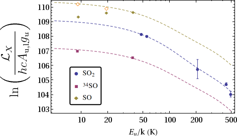
Figure 11: Boltzmann plot of the SO, ³⁴SO, and SO₂ molecular line emission associated with G345.49+1.47. Dashed lines represent fits using two independent thin-SET models, with the same two temperatures fitted to the ³⁴SO and SO₂ transitions. The model for SO was derived from the ³⁴SO data, assuming the same temperatures and the isotopic ratio [³²S/³⁴S]$=22.5$. Empty diamond symbols are the opacity-corrected SO values.

Departures from optically thin predictions are expected for lines whose opacity is greater than 1, and this may be so for the strong SO transitions. We evaluate this possibility by comparing the transitions $3_{2}\rightarrow 2_{1}$ and $4_{5}\rightarrow 4_{4}$ of ³⁴SO and ³²SO. For two isotopologues under SET conditions, the integrated line quotient between two matching transitions is given by

$$\frac{W_{1}}{W_{2}}=\frac{1-e^{-\tau_{1}}}{1-e^{-\tau_{2}}}~{}~{},$$ (20)

where the optical depths are averaged in the line and the ratio $\tau_{1}/\tau_{2}$ is approximately equal to the abundance ratio between the isotopologues. The right side of Equation (20) approaches the opacity ratio under optically thin conditions and approaches 1 in the optically thick limit (Guzmán, 2012, § 3.3.1). We assume that the abundance ratio between the ³²SO and ³⁴SO isotopologues is equal to the terrestrial abundance ratio of the sulfur isotopes, that is, [³²S/³⁴S]$=22.5$. The line ratio of the $3_{2}\rightarrow 2_{1}$ and $4_{5}\rightarrow 4_{4}$ transition and derived ³²SO opacities are

$$\begin{split}W_{\rm{}^{32}SO}/W_{\rm{}^{34}SO}~{}~{}3_{2}\rightarrow 2_{1}&=10.9\Longrightarrow\tau_{32}=1.8\\ W_{\rm{}^{32}SO}/W_{\rm{}^{34}SO}~{}~{}4_{5}\rightarrow 4_{4}&=24.1\Longrightarrow\tau_{32}\ll 1~{}~{}.\end{split}$$ (21)

A simple opacity correction can be applied to the optically thin model by multiplying the right side of Equation (19) by $(1-\exp{(-\tau)})/\tau$, where $\tau$ is the line’s optical depth (Goldsmith & Langer, 1999). We estimate the opacities of the SO $3_{2}\rightarrow 2_{1}$ and $4_{5}\rightarrow 4_{4}$ lines from Equation (21), and that of $2_{2}\rightarrow 1_{1}$ line from the SET model assuming the isotopic abundance ratio [³²S/³⁴S]$=22.5$. The yellow dashed line in Figure 11 displays the prediction of the right side of Equation (19) for SO. Empty diamonds in Figure 11 indicate the opacity-corrected parameters of the SO lines, which we find consistent with the SET model under the assumed isotopic abundance ratio. As derived in Equation (21), no correction is associated with the $4_{5}\rightarrow 4_{4}$ optically thin transition. We emphasize that the SO lines were not used to derive the SET model (dashed lines).

To conclude, we mention that the temperature derived from the two OCS transitions is $\sim 40$ K. It is similar to the warm component temperature determined for the sulfur oxides, but as remarked in the previous section, OCS does not trace the disklike rotating structure. Apparently, at the physical scales probed by our observations (3000 AU, see next section), both a rotating and a presumably larger non-rotating envelope coexist.

4.5.3 Dynamics of the molecular emission

Figure 12 shows the position-velocity (PV) diagram measured from the SO₂ $8_{3,5}\rightarrow 9_{2,8}$ emission. The direction of the PV line is perpendicular to the line indicated in the top left panel of Figure 4 — the jet direction — with zero offset at the position of the jet source. This direction is consistent, within our angular and spectral resolution, with the direction of the largest velocity gradient. It supports the interpretation that the molecular structure probed by our observations is part of a rotating structure with angular momentum direction aligned with the jet axis.

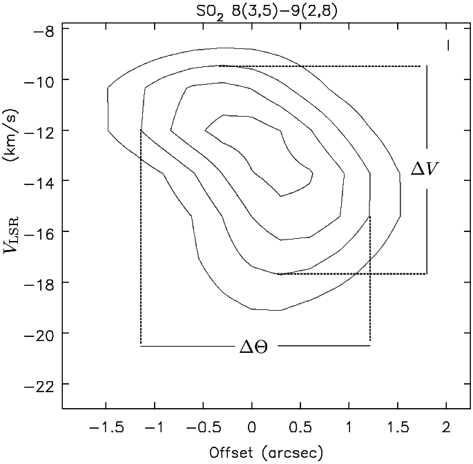
Figure 12: Contour map of the position velocity diagram of the SO₂ $8_{3,5}\rightarrow 9_{2,8}$ emission taken across the direction with P.A.$=8.9$°, through the jet source position (Source 10), averaging 1″ width. The contours correspond to 30, 50, 70, and 90% of the peak equal to 79.2 mJy beam^-1. $\Delta V$ and $\Delta\Theta$ correspond to the extension of the 50% contour in velocity and angular size, respectively.

In order to estimate a dynamical mass, we assume that the disklike structure is centrifugally supported against the gravity of a central mass. We estimate the dynamical mass from the following simplified version of Equation (1) from Franco-Hernández et al. (2009)

$$M_{\star,{\rm dyn}}=\frac{(\sqrt{\Delta\Theta^{2}-\theta_{b}^{2}})\,d}{2G\sin^{2}(i)}\left(\frac{\Delta V}{2}\right)^{2}~{}~{},$$ (22)

where $\Delta\Theta$ is the source size, $\Delta V$ is the velocity breadth, $d$ is the distance, $i$ is the inclination of the disk axis with respect to the line of sight, and $\theta_{b}$ is the beam size. From the 50% contour of the PV diagram shown in Figure 12, we estimate $\Delta\Theta=2\farcs 5$ and $\Delta V=8~{}\mbox{km~{}s${}^{-1}$}$. Using a distance of 1.7 kpc, $\theta_{b}=1\farcs 7$, and an inclination of 45° (Guzmán et al., 2010), we derive a dynamical mass of $56\mbox{$\,M_{\sun}$}$. The approximate physical size of the rotating core, given by $\sqrt{\Delta\Theta^{2}-\theta_{b}^{2}}\,d$, is $3000$ AU. We obtain the same results using instead the SO₂ $7_{3,5}\rightarrow 8_{2,6}$ transition.

4.6 Gentle photo-ionized wind and rotating molecular core toward the HMYSO G345.49+1.47

Our HRL observations indicate that the ionized gas toward G345.49+1.47 is not moving at a very high velocity ($\sim 500$ km s^-1), as observed toward similar objects such as the Cepheus A HW2 jet (Jiménez-Serra et al., 2011). As shown in §4.3.1, Voigt profiles fit the data adequately and they relate naturally with the simple physical model presented in §4.4.2. In principle, however, the HRLs’ wing emission could be produced by high-velocity outflowing gas analogous to the way molecular line wings trace molecular outflows. Line-wing models of outflows are sufficiently flexible to allow for any decay exponents between $-1$ and $-4$ (e.g., Masson & Chernin, 1992; Downes & Cabrit, 2003; Smith et al., 1997), and molecular outflow observations find a distribution of decay exponents also covering this range (Richer et al., 2000). It would be fortuitous, however, if the ionized wings produced by entraining ambient gas had a Lorentz-like and a symmetric shape. Furthermore, between the red- and blue-shifted wing emission we detect no shift in the peak position larger than 0$\farcs$2, an upper boundary limited by our angular resolution (see §3.2).

Four symmetrically aligned ionized lobes seem to be associated with the ionized wind of G345.49+1.47 (Guzmán et al., 2010). If these radio lobes trace shocked-ionized gas, they must trace high-velocity shocks. Proper motion studies have confirmed that radio-lobes associated with objects similar to G345.49+1.47 move rapidly, determining velocities close to $500$ km s^-1 (Martí et al., 1998; Curiel et al., 2006; Rodríguez et al., 2008). Accordingly, it has been often assumed in the literature (e.g. Garay et al., 2003; Su et al., 2004; Bronfman et al., 2008; Guzmán et al., 2010, 2011; Carrasco-González et al., 2012; Johnston et al., 2013) that the continuum ionized source detected toward the center of such systems is tracing high-velocity ionized gas, and even when no lobes are apparent. In view of the results presented in this work toward G345.49+1.47, these assumptions do not seem to be justified unless supported by complementary HRL data.

The dynamical mass determined in § 4.5.3 ($56\mbox{$\,M_{\sun}$}$) is larger than that of a single high-mass star producing the total luminosity of IRAS 16562$-$3959 ($70,000\mbox{$\,L_{\sun}$}$, $25\mbox{$\,M_{\sun}$}$) or the $15\mbox{$\,M_{\sun}$}$ estimated for the dominant HMYSO. Could the rest of the mass, $30\text{-}40\mbox{$\,M_{\sun}$}$ or more, be in the molecular gas phase? This is not likely for two reasons. First, most of the 92 GHz emission comes from ionized gas, with at most $\sim 11$ mJy attributable to dust emission. This is justified in § 4.2, but also by the HRLs’ line intensities, which are consistent with the continuum. This flux corresponds to only 4 $\,M_{\sun}$ assuming 50 K (ref. § 4.5.2), a dust absorption coefficient of $0.3$ cm² g^-1 (extrapolated from the coagulated dust tables of Ormel et al., 2011), a gas-to-dust mass ratio of 100, and optically thin conditions. Second, comparing the total number of SO₂ molecules in the core, more than $30\mbox{$\,M_{\sun}$}$ of molecular gas imply an [SO₂/H] abundance $<6\times 10^{-9}$, which seems low compared with the results of Wakelam et al. (2011). We concede, however, that the SO₂ is expected to vary greatly and this is not an stringent constraint. We conclude that it is more probable that there are (likely more than one) protostellar companions together with the central star. Other compact components will need higher angular resolution studies to be resolved.

Even though there is no evidence from the observed HRLs to suggest that the ionized gas is moving, it is unlikely to be in hydrostatic equilibrium. A coherent model for G345.49+1.47 is that of a pressure-accelerated photo-ionized wind, whose main characteristics can be approximated by a transonic Parker wind (Lamers & Cassinelli, 1999, § 3.1.3) within a conical aperture (Lugo et al., 2004; Keto, 2007). In the Parker wind, the velocity of gas increases very slowly with distance, following $(v/a)\approx\sqrt{\ln(r/r_{c})}$, with $r_{c}=GM_{\star}/2a^{2}$ and $a=9.8~{}\mbox{km~{}s${}^{-1}$}$ is the isothermal sound speed of a solar composition ionized gas at 7000 K. The $\epsilon=1$ conical model presented in § 4.4 is a rough approximation to this solution, since it is conical and has the most shallow acceleration law compared to models with a different geometry ($\epsilon<1$). The acceleration exponent (Equation 8) takes the form $q_{v}=0.97-0.53\epsilon$, as derived from Equation (13) and mass conservation. It remains to be seen what would be the effects of the inclusion of low wind velocities in the line radiation transfer.

The wind collimation derived from the model is $\sim 3$ (§ 4.4.2), which is not high but nevertheless is comparable to the collimation derived from deconvolved resolved radio sources believed to be thermal jets, such as NGC 7538 IRS1 (Sandell et al., 2009), AFGL 2591 (Johnston et al., 2013), Cep A HW2 (Curiel et al., 2006), and G343.1262$-$00.0620 (Rodríguez et al., 2005). In addition, the presence of aligned radio lobes in some cases allows us to infer a more collimated wind such as in G343.1262$-$00.0620 and G345.49+1.47. However, what appears to be clear, at least for G345.49+1.47, is that the hypothetical highly collimated fast jet that excites the ionized lobes does not correspond to the central radio continuum source. For the moment, there are no proper motion measurements toward the lobes of G345.49+1.47, but if they are rapidly moving ($>300$ km s^-1, as in G343.1262$-$00.0620, Cep A, and HH 80-81), it would confirm that the “Jet” source of Guzmán et al. (2010) and the lobes are not linked in the way previously thought.

An interesting possibility is that the ionized wind is analogous to the wide angle low-velocity component observed toward low-mass protostellar jets (Torrelles et al., 2011, and references therein). It is possible that inside this slow ionized wind exists a much narrower, denser, and faster jet, powered by accretion, and responsible for the excitation of the radio lobes. The analogy should not be taken very far, however, since low-mass stars do not produce photo-ionized winds.

5 SUMMARY

We made observations at frequencies 85-99 GHz using ALMA of the continuum, HRLs, and sulfuretted molecular lines toward the massive molecular clump IRAS 16562$-$3959, which harbors the HMYSO G345.49+1.47. The main results are summarized as follows:

1. We detect spatially unresolved emission in the H40$\alpha$, H42$\alpha$, and H50$\beta$ HRLs toward the collimated ionized wind source associated with G345.49+1.47. The lines display Voigt profiles with Lorentzian wings of widths between 30 and 40 km s^-1, which we interpret as pressure broadening arising from ionized gas with average density of $5\times 10^{7}$ cm^-3.

2. A parameterized model of a slow ionized wind is sufficient to simultaneously fit the HRLs and the continuum emission between 1 and 100 GHz associated with G345.49+1.47. There is no need for ionized gas moving at velocities in excess of 50 km s^-1in order to explain the HRL profiles.

3. We detect in the ALMA field of view ($\sim 1\arcmin$) at least 15 additional continuum sources, probably associated with the IRAS 16562$-$3959 clump, with spectra consistent with part of the emission arising from optically thin dust. These sources are likely to correspond to dusty molecular cores.

4. The emission in the SO₂, ³⁴SO, and SO lines with upper energy levels $\leq 50$ K exhibits velocity gradients that we interpret as arising from a rotating compact ($\sim 3000$ AU) molecular core with angular momentum aligned with the jet axis. The estimated dynamical mass is $56\mbox{$\,M_{\sun}$}$.

5. Sulfuretted molecular emission associated with the core has excitation temperatures that range between 35 and 140 K.

6. Qualitatively, the SO, SO₂, and CS emission and morphology can be understood using the predictions of hot gaseous phase chemical models (e.g., Charnley 1997 and van der Tak et al. 2003). Additional irradiated ice-chemistry might be necessary to explain the characteristics of the OCS emission.

7. G345.49+1.47 is a $\sim 15\mbox{$\,M_{\sun}$}$ HMYSO associated with a photo-ionized wind that dominates the free-free emission. It is likely that within this photo-ionized wind, a highly collimated jet is powered by an accretion disk, responsible for the excitation of the aligned radio lobes.

Appendix A Continuum flux expected from the jet model

Assuming that the Rayleigh-Jeans approximation is valid at the frequencies of interest ($B_{\nu}(T)\approx 2kT\nu^{2}/c^{2}$) and that all relevant quantities along a line of sight through the jet are given by their values at the jet axis (see Figure 9), the radio continuum flux density from the whole jet system (jet+counterjet) can be written approximately as (see Equations 7 and 8 from Reynolds 1986)

$$S_{\nu} =2\times\int_{y_{\rm i}}^{y_{\rm f}}\frac{2kT(y)\nu^{2}}{c^{2}}\frac{2w(y)}{d^{2}}\left(1-\exp(-\tau(\nu,y))\right)dy$$

$$=2\times\frac{2kT_{0}\nu^{2}}{c^{2}}\frac{2w_{0}y_{0}}{d^{2}}\int_{y_{\rm i}}^{y_{\rm f}}\left(\frac{y}{y_{0}}\right)^{\epsilon+q_{T}}\left(1-\exp\left(-\tau_{0}(\nu)\,(y/y0)^{q_{\tau}}\right)\right)\frac{dy}{y_{0}}~{}~{}.$$

The extra factor 2 with respect to the equations in Reynolds (1986) takes into account the emission from the two sides of the jet. Note that $(r/r_{0})=(y/y_{0})$, making it trivial to change the dependence on $r$ to a dependence on $y$. Defining $\Omega_{0}=2w_{0}y_{0}/d^{2}$ and making the change of variable $u=y/y_{0}$, we obtain

$$S_{\nu}=2\times B_{\nu}(T_{0})\Omega_{0}\int_{u_{\rm i}}^{u_{\rm f}}u^{\epsilon+q_{T}}\left(1-\exp\left(-\tau_{0}(\nu)\,u^{q_{\tau}}\right)\right)du~{}~{},$$ (A1)

which, after the following change of variable, $\tau=\tau_{0}(\nu)u^{q_{\tau}}$ (note that $q_{\tau}<0$), becomes

$$S_{\nu}=2\times B_{\nu}(T_{0})\Omega_{0}\left(\tau_{0}(\nu)\right)^{-\frac{\epsilon+q_{T}+1}{q_{\tau}}}\int_{\tau_{\rm f}}^{\tau_{\rm i}}\tau^{\frac{\epsilon+q_{T}+1}{q_{\tau}}-1}\left(1-\exp(-\tau)\right)\frac{d\tau}{(-q_{\tau})}~{}~{}.$$ (A2)

In this way, the integral over the source extension in the sky is re-written as an integral over the values taken by the continuum opacity. Equation (A2) gives us the flux density of the source, which is the only quantity we can actually probe since we do not resolve the jet structure.

Defining $\eta:=(1+\epsilon+q_{T})/q_{\tau}$ (called “$c$” in Reynolds 1986), we finally obtain

$$S_{\nu}=2\times B_{\nu}(T_{0})\Omega_{0}\frac{(\tau_{0})^{-\eta}}{(-q_{\tau})}\left(\frac{\tau_{\rm i}^{\eta}-\tau_{\rm f}^{\eta}}{\eta}+\Gamma(\eta,\tau_{\rm i})-\Gamma(\eta,\tau_{\rm f})\right)~{}~{},$$ (A3)

where $\Gamma(\eta,\tau):=\int_{\tau}^{\infty}t^{\eta-1}e^{-t}dt$ is the incomplete Gamma function. Note that the frequency dependence is in the Planck function and on the optical depth. The reason for changing to this formalism is that under the limit $\tau_{i}\rightarrow\infty$ and $\tau_{e}\rightarrow 0$ (valid for the frequencies where we see the spectrum is a power law), Equation (A3) simplifies to

$$S_{\nu}=2\times B_{\nu}(T_{0})\Omega_{0}\frac{\Gamma(\eta)}{q_{\tau}}(\tau_{0}(\nu))^{-\eta}~{}~{},$$ (A4)

where $\Gamma(\eta)$ is the Gamma function evaluated for $\eta$. No assumption regarding the dependence of the opacity on frequency has been made. If we assume that $\tau_{0}(\nu)\propto\nu^{-2.1}$ — a valid approximation for the frequencies of interest — we get the Equation (13) for the spectral index, equivalent to

$$\alpha_{op}=2+2.1\eta~{}~{},$$

which is Equation (15) from Reynolds (1986). $\eta$ is a negative number between $-1$ and 0. In particular, when $\alpha_{op}=0.92$, $\eta=-0.51$ and $\Gamma(\eta)<0$ $\left(\Gamma(-0.51)\approx-2\sqrt{\pi}\right)$. After introducing a fiducial frequency $\nu_{0}$ and replacing it in Equation (A4), we obtain Equation (12). Equations (A3) and (A4) extend the derivation of Reynolds (1986).

A.1 Morphological constraints

Our observations give little information about the physical scale size of the jet. Both ALMA and the centimeter wavelength observations (Guzmán et al., 2010) indicate that the jet is unresolved, which imply that the optically thick portion does not extend farther than the size of the beam. This condition is equivalent to

$$\bar{y} =d\times\text{FWHM}_{\rm obs}/2$$ (A5)

$$\tau(\bar{y}) =\tau_{0}\left(\frac{\text{FWHM}_{\rm obs}\,d}{2r_{0}\sin i}\right)^{q_{\tau}}<1\qquad\text{(From Equation \ref{proj-height}.)}$$ (A6)

where $\text{FWHM}_{\rm obs}$ is the full-width at half-maximum of the synthesized beam. It turns out that the most stringent constraint is given by the ATCA data at 8.6 GHz. All the models consistent with the data easily fulfill Equation (A6).

Appendix B Line flux expected from the jet model

To derive the expected HRLs, we start in Equation (A1), which is also valid for the emission at the frequencies of the lines, taking into account that the optical depth includes the continuum and line contributions. The equation for the total flux (continuum+recombination line) is

$$S_{\rm\nu,L+C}=2\times B_{\nu}(T_{0})\Omega_{0}\int_{u_{\rm i}}^{u_{\rm f}}u^{\epsilon+q_{T}}\left(1-\exp\left(-\tau(\nu,u)\right)\right)du~{}~{},$$ (B1)

where the integration is over $u=y/y_{0}$ (see Figure 9). The total, continuum, and line optical depths are given across the jet by

$$\tau(\nu,u) =\tau_{C}(\nu,u)+\tau_{L}(\nu,u)~{}~{},$$ (B2)

$$\tau_{\rm C}(\nu,u) =\tau_{\rm C,0}(\nu)u^{q_{\tau}}~{}~{},$$ (B3)

$$\tau_{\rm L}(\nu,u) =\mathcal{T}_{\rm L}(u)\times\phi(\nu,u)~{}~{}.$$ (B4)

In the last equation, $\mathcal{T}_{\rm L}(u)$ represents the integrated optical depth of the line, and we assume that $\int\phi(\nu,u)d\nu=1$. The line profile $\phi(\nu,u)$ depends on the line of sight, parameterized by $u$ in Equation (B1). The integrated optical depth $\mathcal{T}_{\rm L}(u)$ depends on $u$ because it depends on the density ($\propto N_{e}^{2}$) and on the path length. We use the formulae for HRLs described in Gordon & Sorochenko (2002, § 2.3.5),

$$\mathcal{T}_{\rm L}=s(u)\times N_{n}\frac{\alpha h}{2m_{e}}f(n,\Delta n)\left(1-e^{-h\nu_{\rm L}/kT_{e}}\right)~{}~{},$$ (B5)

where $s(u)$ is the path length, $N_{n}$ is the population in the $n$ quantum level, $\nu_{L}$ corresponds to the rest frequency of the line associated with the $(n+\Delta n)\rightarrow n$ transition, and the rest of the physical constants, including $\alpha\approx 137^{-1}$, are in the usual notation. The oscillator strength of the line, $f(n,\Delta n)$, is given by

$$f(n,\Delta n)=n\mathcal{M}(\Delta n)\left(1+1.5\frac{\Delta n}{n}\right)~{}~{},$$

where $\mathcal{M}(1)=0.190775$ and $\mathcal{M}(2)=0.026332$ are the Menzel constants (Menzel, 1968). The population level $N_{n}$ under LTE is given by the Saha-Boltzmann ionization equation,

$$N_{n}=N_{e}^{2}\frac{n^{2}h^{3}}{(2\pi m_{e}kT_{e})^{3/2}}\exp\left(\frac{m_{e}c^{2}}{2kT_{e}}\left(\frac{\alpha}{n}\right)^{2}\frac{m_{H}}{m_{e}+m_{H}}\right)~{}~{},$$ (B6)

assuming a purely hydrogen gas with $m_{H}$ being the hydrogen mass. Note that the statistical weight associated with degeneracy of the $n$-th level, $g_{n}=n^{2}$, is already included.

As in the appendix for the continuum, we assume that all relevant quantities along a line of sight through the jet are given by their values at the jet axis.

Note that the optical depth of the continuum and the integrated optical depth $\mathcal{T}_{\rm L}$ are both proportional to $N_{e}^{2}$ and to the path length $s$ (see Figure 9). Therefore, the quotient $\mathcal{T}_{\rm L}/\tau_{\rm C}$ is independent of density and path length and depends only on $T_{e}$. Under the assumption of isothermality, it is also independent of the integration variable in Equation (B1). We call this quotient the equivalent line width of the transition, defined by $\Delta\nu_{\rm L}:=\mathcal{T}_{\rm L}/\tau_{\rm C}$. The value of $\Delta\nu_{\rm L}$ for the HRLs observed in this work is given in Equation (15). We remark that these are not truly line widths, but a measure of the area of the line compared to the continuum level.

Then, we change the variable of integration to the continuum opacity using

$$\begin{split}\tau(\nu,u)&=\tau_{\rm C}(\nu,u)+\tau_{\rm L}(\nu,u)\\ &=\tau_{\rm C}(\nu,u)\left(1+\Delta\nu_{\rm L}\phi(\nu,u)\right)\\ &=\tau_{\rm C,0}(\nu)u^{q_{\tau}}\left(1+\Delta\nu_{\rm L}\phi(\nu,u)\right)~{}~{}.\end{split}$$ (B7)

This allows us to calculate the limit $\tau_{i}\rightarrow\infty$ and $\tau_{e}\rightarrow 0$, which is the same procedure used to derive Equation (12). Therefore, Equation (B1) takes the following form,

$$S_{\rm\nu,L+C}=2\times B_{\nu}(T_{0})\Omega_{0}\frac{(\tau_{\rm C,0})^{-\eta}}{(-q_{\tau})}\int_{0}^{\infty}\tau^{\eta-1}\left(1-e^{-\tau(1+\Delta\nu_{\rm L}\phi(\nu,\tau))}\right)d\tau~{}~{},$$ (B8)

where $\eta=(\alpha_{\rm op}-2)/2.1$. Combining the previous equation with Equation (12), we determine that the line flux $S_{\rm L}=S_{\rm L+C}-S_{\rm C}$ is given by

$$\begin{split}S_{\rm\nu,L}&=S_{\rm\nu,C}\left(\frac{\int_{0}^{\infty}\tau^{\eta-1}\left(1-e^{-\tau(1+\Delta\nu_{\rm L}\phi(\nu,\tau))}\right)d\tau}{-\Gamma(\eta)}-1\right)\\ &=S_{\rm\nu_{0},C}\left(\frac{\nu}{\nu_{0}}\right)^{\alpha_{op}}\left(\frac{\int_{0}^{\infty}\tau^{\eta-1}\left(1-e^{-\tau(1+\Delta\nu_{\rm L}\phi(\nu,\tau))}\right)d\tau}{-\Gamma(\eta)}-1\right)~{}~{},\end{split}$$ (B9)

which gives the line flux density predicted for HRLs in LTE from the ionized jet model presented in the previous section. Equation (B9) corresponds to Equation (14).

References

- Alexander & Gulyaev (2012) Alexander, J., & Gulyaev, S. 2012, ApJ, 745, 194
- Anglada (1996) Anglada, G. 1996, in Astronomical Society of the Pacific Conference Series, Vol. 93, Radio Emission from the Stars and the Sun, ed. A. R. Taylor & J. M. Paredes, 3–7
- Báez-Rubio et al. (2013) Báez-Rubio, A., Martín-Pintado, J., Thum, C., & Planesas, P. 2013, A&A, 553, A45
- Bell et al. (2000) Bell, M. B., Avery, L. W., Seaquist, E. R., & Vallée, J. P. 2000, PASP, 112, 1236
- Beltrán et al. (2006) Beltrán, M. T., Cesaroni, R., Codella, C., Testi, L., Furuya, R. S., & Olmi, L. 2006, Nature, 443, 427
- Beltrán et al. (2011) Beltrán, M. T., Cesaroni, R., Neri, R., & Codella, C. 2011, A&A, 525, A151
- Benjamin et al. (2003) Benjamin, R. A., et al. 2003, PASP, 115, 953
- Beuther et al. (2007) Beuther, H., Leurini, S., Schilke, P., Wyrowski, F., Menten, K. M., & Zhang, Q. 2007, A&A, 466, 1065
- Beuther et al. (2013) Beuther, H., Linz, H., & Henning, T. 2013, A&A, 558, A81
- Beuther et al. (2002) Beuther, H., Schilke, P., Sridharan, T. K., Menten, K. M., Walmsley, C. M., & Wyrowski, F. 2002, A&A, 383, 892
- Blandford & Payne (1982) Blandford, R. D., & Payne, D. G. 1982, MNRAS, 199, 883
- Briggs (1995) Briggs, D. S. 1995, PhD thesis, New Mexico Institute of Mining and Technology, USA
- Bronfman et al. (2008) Bronfman, L., Garay, G., Merello, M., Mardones, D., May, J., Brooks, K. J., Nyman, L.-Å., & Güsten, R. 2008, ApJ, 672, 391
- Bronfman et al. (1996) Bronfman, L., Nyman, L.-A., & May, J. 1996, A&AS, 115, 81
- Brown et al. (1978) Brown, R. L., Lockman, F. J., & Knapp, G. R. 1978, ARA&A, 16, 445
- Cabrit (2007) Cabrit, S. 2007, in Lecture Notes in Physics, Berlin Springer Verlag, Vol. 723, Jets from Young Stars I: Models and Constraints, ed. J. Ferreira, C. Dougados, & E. Whelan, 21–50
- Carrasco-González et al. (2010) Carrasco-González, C., Rodríguez, L. F., Torrelles, J. M., Anglada, G., & González-Martín, O. 2010, AJ, 139, 2433
- Carrasco-González et al. (2012) Carrasco-González, C., et al. 2012, ApJ, 752, L29
- Caswell (1998) Caswell, J. L. 1998, MNRAS, 297, 215
- Cesaroni et al. (1997) Cesaroni, R., Felli, M., Testi, L., Walmsley, C. M., & Olmi, L. 1997, A&A, 325, 725
- Charnley (1997) Charnley, S. B. 1997, ApJ, 481, 396
- Curiel et al. (1989) Curiel, S., Rodriguez, L. F., Bohigas, J., Roth, M., Canto, J., & Torrelles, J. M. 1989, Astrophysical Letters and Communications, 27, 299
- Curiel et al. (2006) Curiel, S., et al. 2006, ApJ, 638, 878
- De Biévre & Taylor (1993) De Biévre, P., & Taylor, P. D. P. 1993, International Journal of Mass Spectrometry and Ion Processes, 123, 149
- De Young (1991) De Young, D. S. 1991, Science, 252, 389
- Downes & Cabrit (2003) Downes, T. P., & Cabrit, S. 2003, A&A, 403, 135
- Draine (2006) Draine, B. T. 2006, ApJ, 636, 1114
- Dubernet et al. (2013) Dubernet, M.-L., et al. 2013, A&A, 553, A50
- Fallscheer et al. (2011) Fallscheer, C., Beuther, H., Sauter, J., Wolf, S., & Zhang, Q. 2011, ApJ, 729, 66
- Faúndez et al. (2004) Faúndez, S., Bronfman, L., Garay, G., Chini, R., Nyman, L.-Å., & May, J. 2004, A&A, 426, 97
- Fazio et al. (2004) Fazio, G. G., et al. 2004, ApJS, 154, 10
- Feigelson & Babu (2012) Feigelson, E., & Babu, G. 2012, Modern Statistical Methods for Astronomy: With R Applications (Cambridge University Press)
- Fernández-López et al. (2011) Fernández-López, M., Girart, J. M., Curiel, S., Gómez, Y., Ho, P. T. P., & Patel, N. 2011, AJ, 142, 97
- Ferrante et al. (2008) Ferrante, R. F., Moore, M. H., Spiliotis, M. M., & Hudson, R. L. 2008, ApJ, 684, 1210
- Foster et al. (2007) Foster, T. J., Kothes, R., Kerton, C. R., & Arvidsson, K. 2007, ApJ, 667, 248
- Franco-Hernández et al. (2009) Franco-Hernández, R., Moran, J. M., Rodríguez, L. F., & Garay, G. 2009, ApJ, 701, 974
- Frank et al. (2014) Frank, A., et al. 2014, ArXiv e-prints
- Galván-Madrid et al. (2012) Galván-Madrid, R., Goddi, C., & Rodríguez, L. F. 2012, A&A, 547, L3
- Galván-Madrid et al. (2010) Galván-Madrid, R., Zhang, Q., Keto, E., Ho, P. T. P., Zapata, L. A., Rodríguez, L. F., Pineda, J. E., & Vázquez-Semadeni, E. 2010, ApJ, 725, 17
- Garay (2005) Garay, G. 2005, in IAU Symposium, Vol. 227, Massive Star Birth: A Crossroads of Astrophysics, ed. R. Cesaroni, M. Felli, E. Churchwell, & M. Walmsley, 86–91
- Garay et al. (2003) Garay, G., Brooks, K. J., Mardones, D., & Norris, R. P. 2003, ApJ, 587, 739
- Garay et al. (2002) Garay, G., Brooks, K. J., Mardones, D., Norris, R. P., & Burton, M. G. 2002, ApJ, 579, 678
- Garay et al. (2007) Garay, G., et al. 2007, A&A, 463, 217
- Garden et al. (1991) Garden, R. P., Hayashi, M., Hasegawa, T., Gatley, I., & Kaifu, N. 1991, ApJ, 374, 540
- Gibb et al. (2003) Gibb, A. G., Hoare, M. G., Little, L. T., & Wright, M. C. H. 2003, MNRAS, 339, 1011
- Gibb et al. (2004) Gibb, E. L., Whittet, D. C. B., Boogert, A. C. A., & Tielens, A. G. G. M. 2004, ApJS, 151, 35
- Goldsmith & Langer (1999) Goldsmith, P. F., & Langer, W. D. 1999, ApJ, 517, 209
- Gordon & Sorochenko (2002) Gordon, M. A., & Sorochenko, R. L. 2002, Astrophysics and Space Science Library, Vol. 282, Radio Recombination Lines. Their Physics and Astronomical Applications (Springer-Verlag)
- Green & Chapman (1978) Green, S., & Chapman, S. 1978, ApJS, 37, 169
- Griem (1967) Griem, H. R. 1967, ApJ, 148, 547
- Guzmán (2012) Guzmán, A. E. 2012, PhD thesis, Universidad de Chile
- Guzmán et al. (2010) Guzmán, A. E., Garay, G., & Brooks, K. J. 2010, ApJ, 725, 734
- Guzmán et al. (2011) Guzmán, A. E., Garay, G., Brooks, K. J., Rathborne, J., & Güsten, R. 2011, ApJ, 736, 150
- Guzmán et al. (2012) Guzmán, A. E., Garay, G., Brooks, K. J., & Voronkov, M. A. 2012, ApJ, 753, 51
- Hatchell et al. (1998) Hatchell, J., Thompson, M. A., Millar, T. J., & MacDonald, G. H. 1998, A&A, 338, 713
- Herpin et al. (2009) Herpin, F., Marseille, M., Wakelam, V., Bontemps, S., & Lis, D. C. 2009, A&A, 504, 853
- Ho & Haschick (1986) Ho, P. T. P., & Haschick, A. D. 1986, ApJ, 304, 501
- Hoare & Franco (2007) Hoare, M. G., & Franco, J. 2007, in Diffuse Matter from Star Forming Regions to Active Galaxies, ed. Hartquist, T. W., Pittard, J. M., & Falle, S. A. E. G., 61
- Hosokawa & Omukai (2009) Hosokawa, T., & Omukai, K. 2009, ApJ, 691, 823
- Hudson & Moore (2000) Hudson, R. L., & Moore, M. H. 2000, A&A, 357, 787
- Hunter et al. (2014) Hunter, T. R., Brogan, C. L., Cyganowski, C. J., & Young, K. H. 2014, ApJ, 788, 187
- Jaffe & Martín-Pintado (1999) Jaffe, D. T., & Martín-Pintado, J. 1999, ApJ, 520, 162
- Jiménez-Serra et al. (2011) Jiménez-Serra, I., Martín-Pintado, J., Báez-Rubio, A., Patel, N., & Thum, C. 2011, ApJ, 732, L27
- Jiménez-Serra et al. (2012) Jiménez-Serra, I., Zhang, Q., Viti, S., Martín-Pintado, J., & de Wit, W.-J. 2012, ApJ, 753, 34
- Johnston et al. (2013) Johnston, K. G., Shepherd, D. S., Robitaille, T. P., & Wood, K. 2013, A&A, 551, A43
- Keto (2007) Keto, E. 2007, ApJ, 666, 976
- Keto & Klaassen (2008) Keto, E., & Klaassen, P. 2008, ApJ, 678, L109
- Keto & Wood (2006) Keto, E., & Wood, K. 2006, ApJ, 637, 850
- Keto et al. (2008) Keto, E., Zhang, Q., & Kurtz, S. 2008, ApJ, 672, 423
- Kraus et al. (2010) Kraus, S., et al. 2010, Nature, 466, 339
- Kuiper et al. (2011) Kuiper, R., Klahr, H., Beuther, H., & Henning, T. 2011, ApJ, 732, 20
- Lada & Lada (2003) Lada, C. J., & Lada, E. A. 2003, ARA&A, 41, 57
- Lamers & Cassinelli (1999) Lamers, H. J. G. L. M., & Cassinelli, J. P. 1999, Introduction to Stellar Winds (Cambridge University Press)
- Lampton et al. (1976) Lampton, M., Margon, B., & Bowyer, S. 1976, ApJ, 208, 177
- Lang (1999) Lang, K. 1999, Astrophysical Formulae (Springer)
- Larson (2003) Larson, R. B. 2003, in Astronomical Society of the Pacific Conference Series, Vol. 287, Galactic Star Formation Across the Stellar Mass Spectrum, ed. J. M. De Buizer & N. S. van der Bliek, 65–80
- Li et al. (2014) Li, Z.-Y., Banerjee, R., Pudritz, R. E., Jørgensen, J. K., Shang, H., Krasnopolsky, R., & Maury, A. 2014, ArXiv e-prints
- Livio (2009) Livio, M. 2009, in Protostellar Jets in Context, ed. Tsinganos, K., Ray, T., & Stute, M., 3–9
- López et al. (2011) López, C., Bronfman, L., May, J., Nyman, L.-A., & Garay, G. 2011, A&A, 534, A131
- Lugo et al. (2004) Lugo, J., Lizano, S., & Garay, G. 2004, ApJ, 614, 807
- Lumsden et al. (2013) Lumsden, S. L., Hoare, M. G., Urquhart, J. S., Oudmaijer, R. D., Davies, B., Mottram, J. C., Cooper, H. D. B., & Moore, T. J. T. 2013, ApJS, 208, 11
- Lumsden et al. (2012) Lumsden, S. L., Wheelwright, H. E., Hoare, M. G., Oudmaijer, R. D., & Drew, J. E. 2012, MNRAS, 424, 1088
- Maity & Kaiser (2013) Maity, S., & Kaiser, R. I. 2013, ApJ, 773, 184
- Martí et al. (1993) Martí, J., Rodríguez, L. F., & Reipurth, B. 1993, ApJ, 416, 208
- Martí et al. (1998) —. 1998, ApJ, 502, 337
- Martins et al. (2005) Martins, F., Schaerer, D., & Hillier, D. J. 2005, A&A, 436, 1049
- Masson & Chernin (1992) Masson, C. R., & Chernin, L. M. 1992, ApJ, 387, L47
- Maud et al. (2013) Maud, L. T., Hoare, M. G., Gibb, A. G., Shepherd, D., & Indebetouw, R. 2013, MNRAS, 428, 609
- Menzel (1968) Menzel, D. H. 1968, Nature, 218, 756
- Mezger & Palmer (1968) Mezger, P. G., & Palmer, P. 1968, Science, 160, 29
- Müller et al. (2001) Müller, H. S. P., Thorwirth, S., Roth, D. A., & Winnewisser, G. 2001, A&A, 370, L49
- Ormel et al. (2011) Ormel, C. W., Min, M., Tielens, A. G. G. M., Dominik, C., & Paszun, D. 2011, A&A, 532, A43
- Paladini et al. (2004) Paladini, R., Davies, R. D., & De Zotti, G. 2004, MNRAS, 347, 237
- Patel et al. (2005) Patel, N. A., et al. 2005, Nature, 437, 109
- Peters et al. (2012) Peters, T., Longmore, S. N., & Dullemond, C. P. 2012, MNRAS, 425, 2352
- Petry & CASA Development Team (2012) Petry, D., & CASA Development Team. 2012, in Astronomical Society of the Pacific Conference Series, Vol. 461, Astronomical Data Analysis Software and Systems XXI, ed. P. Ballester, D. Egret, & N. P. F. Lorente, 849
- Pickett et al. (1998) Pickett, H. M., Poynter, R. L., Cohen, E. A., Delitsky, M. L., Pearson, J. C., & Müller, H. S. P. 1998, J. Quant. Spec. Radiat. Transf., 60, 883
- Qiu et al. (2012) Qiu, K., Zhang, Q., Beuther, H., & Fallscheer, C. 2012, ApJ, 756, 170
- Ray et al. (2007) Ray, T., Dougados, C., Bacciotti, F., Eislöffel, J., & Chrysostomou, A. 2007, Protostars and Planets V, 231
- Remijan et al. (2007) Remijan, A. J., Markwick-Kemper, A., & ALMA Working Group on Spectral Line Frequencies. 2007, in Bulletin of the American Astronomical Society, Vol. 39, American Astronomical Society Meeting Abstracts, 132.11
- Reynolds (1986) Reynolds, S. P. 1986, ApJ, 304, 713
- Richer et al. (2000) Richer, J. S., Shepherd, D. S., Cabrit, S., Bachiller, R., & Churchwell, E. 2000, Protostars and Planets IV, 867
- Robitaille et al. (2007) Robitaille, T. P., Whitney, B. A., Indebetouw, R., & Wood, K. 2007, ApJS, 169, 328
- Rodríguez et al. (2005) Rodríguez, L. F., Garay, G., Brooks, K. J., & Mardones, D. 2005, ApJ, 626, 953
- Rodríguez et al. (1994) Rodríguez, L. F., Garay, G., Curiel, S., Ramírez, S., Torrelles, J. M., Gómez, Y., & Velazquez, A. 1994, ApJ, 430, L65
- Rodriguez et al. (1993) Rodriguez, L. F., Marti, J., Canto, J., Moran, J. M., & Curiel, S. 1993, Rev. Mexicana Astron. Astrofis., 25, 23
- Rodríguez et al. (2008) Rodríguez, L. F., Moran, J. M., Franco-Hernández, R., Garay, G., Brooks, K. J., & Mardones, D. 2008, AJ, 135, 2370
- Sana et al. (2012) Sana, H., et al. 2012, Science, 337, 444
- Sánchez-Monge et al. (2013) Sánchez-Monge, Á., et al. 2013, A&A, 552, L10
- Sandell et al. (2009) Sandell, G., Goss, W. M., Wright, M., & Corder, S. 2009, ApJ, 699, L31
- Sanhueza et al. (2012) Sanhueza, P., Jackson, J. M., Foster, J. B., Garay, G., Silva, A., & Finn, S. C. 2012, ApJ, 756, 60
- Sewiło et al. (2011) Sewiło, M., Churchwell, E., Kurtz, S., Goss, W. M., & Hofner, P. 2011, ApJS, 194, 44
- Shepherd et al. (1998) Shepherd, D. S., Watson, A. M., Sargent, A. I., & Churchwell, E. 1998, ApJ, 507, 861
- Shu et al. (1987) Shu, F. H., Adams, F. C., & Lizano, S. 1987, ARA&A, 25, 23
- Simpson (1973) Simpson, J. P. 1973, Ap&SS, 20, 187
- Skrutskie et al. (2006) Skrutskie, M. F., et al. 2006, AJ, 131, 1163
- Smirnov et al. (1984) Smirnov, G. T., Sorochenko, R. L., & Pankonin, V. 1984, A&A, 135, 116
- Smith et al. (1997) Smith, M. D., Suttner, G., & Yorke, H. W. 1997, A&A, 323, 223
- Stepkin et al. (2007) Stepkin, S. V., Konovalenko, A. A., Kantharia, N. G., & Udaya Shankar, N. 2007, MNRAS, 374, 852
- Strelnitski et al. (1996) Strelnitski, V. S., Ponomarev, V. O., & Smith, H. A. 1996, ApJ, 470, 1118
- Su et al. (2004) Su, Y.-N., Zhang, Q., & Lim, J. 2004, ApJ, 604, 258
- Tan et al. (2014) Tan, J. C., Beltran, M. T., Caselli, P., Fontani, F., Fuente, A., Krumholz, M. R., McKee, C. F., & Stolte, A. 2014, ArXiv e-prints
- Tofani et al. (1995) Tofani, G., Felli, M., Taylor, G. B., & Hunter, T. R. 1995, A&AS, 112, 299
- Torrelles et al. (2011) Torrelles, J. M., et al. 2011, MNRAS, 410, 627
- Vaidya et al. (2011) Vaidya, B., Fendt, C., Beuther, H., & Porth, O. 2011, ApJ, 742, 56
- van der Tak (2011) van der Tak, F. 2011, in IAU Symposium, Vol. 280, IAU Symposium, ed. J. Cernicharo & R. Bachiller, 449–460
- van der Tak et al. (2003) van der Tak, F. F. S., Boonman, A. M. S., Braakman, R., & van Dishoeck, E. F. 2003, A&A, 412, 133
- Villuendas et al. (1996) Villuendas, E., Anglada, G., Estalella, R., Rodríguez, L. V., Curiel, S., & Torrelles, J. M. 1996, in Astronomical Society of the Pacific Conference Series, Vol. 93, Radio Emission from the Stars and the Sun, ed. A. R. Taylor & J. M. Paredes, 56–58
- von Procházka et al. (2010) von Procházka, A. A., et al. 2010, PASP, 122, 354
- Wakelam et al. (2011) Wakelam, V., Hersant, F., & Herpin, F. 2011, A&A, 529, A112
- Walmsley (1990) Walmsley, C. M. 1990, A&AS, 82, 201
- Walmsley (1995) Walmsley, M. 1995, in Revista Mexicana de Astronomia y Astrofisica Conference Series, Vol. 1, Revista Mexicana de Astronomia y Astrofisica Conference Series, ed. S. Lizano & J. M. Torrelles, 137
- Wilson et al. (2009) Wilson, T. L., Rohlfs, K., & Hüttemeister, S. 2009, Tools of Radio Astronomy (Springer-Verlag)
- Wu & Evans (2003) Wu, J., & Evans, II, N. J. 2003, ApJ, 592, L79
- Wu et al. (2004) Wu, Y., Wei, Y., Zhao, M., Shi, Y., Yu, W., Qin, S., & Huang, M. 2004, A&A, 426, 503
- Zapata et al. (2009) Zapata, L. A., Ho, P. T. P., Schilke, P., Rodríguez, L. F., Menten, K., Palau, A., & Garrod, R. T. 2009, ApJ, 698, 1422
- Zhang (2005) Zhang, Q. 2005, in IAU Symposium, Vol. 227, Massive Star Birth: A Crossroads of Astrophysics, ed. R. Cesaroni, M. Felli, E. Churchwell, & M. Walmsley, 135–144
- Zhang & Ho (1997) Zhang, Q., & Ho, P. T. P. 1997, ApJ, 488, 241
- Zhang et al. (2007) Zhang, Q., Hunter, T. R., Beuther, H., Sridharan, T. K., Liu, S.-Y., Su, Y.-N., Chen, H.-R., & Chen, Y. 2007, ApJ, 658, 1152
- Zhang et al. (2005) Zhang, Q., Hunter, T. R., Brand, J., Sridharan, T. K., Cesaroni, R., Molinari, S., Wang, J., & Kramer, M. 2005, ApJ, 625, 864
- Zhang et al. (2001) Zhang, Q., Hunter, T. R., Brand, J., Sridharan, T. K., Molinari, S., Kramer, M. A., & Cesaroni, R. 2001, ApJ, 552, L167
- Zinnecker & Yorke (2007) Zinnecker, H., & Yorke, H. W. 2007, ARA&A, 45, 481