Collective decision making and paradoxical games.

Abstract

We study an ensemble of individuals playing the two games of the so-called Parrondo paradox. In our study, players are allowed to choose the game to be played by the whole ensemble in each turn. The choice cannot conform to the preferences of all the players and, consequently, they face a simple frustration phenomenon that requires some strategy to make a collective decision. We consider several such strategies and analyze how fluctuations can be used to improve the performance of the system.

1 Introduction

Collective decision making is a major topic not only in economics and public choice theory [1], but also in communication, computer science, machine learning, game theory, and control theory. The so-called paradoxical games or Parrondo paradox [2, 3] have provided a simple example of collective decision making exhibiting interesting features, such as the inefficiency of voting [4] and of short-term optimization [5].

The paradox was initially designed as an illustration of Brownian ratchets. However, its simplicity has helped to explore possible applications of the ratchet effect to quantum games [6], quantum decoherence [7], microbial evolution [8, 9], deterministic chaos [10], and stochastic control and optimization [11, 12].

The paradox consists of two losing gambling games, A and B, which yield a winning game when alternated either in a periodic or random way. In the original formulation of the paradox, an individual plays against the casino with the following rules. In game A, the player has a probability $p_{A}=1/2-\epsilon$ of winning one euro and a probability $1-p_{A}=1/2+\epsilon$ of losing one euro, where the bias $\epsilon$ is a small positive number. This game can be considered as a bet of one euro on the toss of a slightly biased coin.

The second game, B, is played with two biased coins, a “bad coin” and a “good coin”. The player must toss the bad coin if her capital $X(t)$ is a multiple of $3$, the probability of winning being $p_{\rm bad}=1/10-\epsilon$. Otherwise, the good coin is tossed and the probability of winning is $p_{\rm good}=3/4-\epsilon$. The rules of games A and B are represented in Fig. 1, in which darkness indicates the “badness” of each coin.

The rules are such that the two games are losing if $\epsilon>0$, i.e., the mean value of the capital $X(t)$ is a decreasing function of the number $t$ of turns played. However, for many random and periodic sequences, such as ABBABBABB…, the capital increases on average.

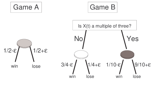
Figure 1: Rules of the paradoxical games.

Recently, the possible relevance of the paradox has been questioned by arguing that it becomes trivial if the player is allowed to choose the game in each turn [13]. This argument is itself quite trivial. The choice is very simple: if $X(t)$ is a multiple of three, one has to choose game A to avoid the use of the bad coin in game B; on the other hand, if $X(t)$ is not a multiple of three, then the best choice is B. With this strategy, the capital is clearly increasing on average. Moreover, this is the optimal strategy for a single player.

However, if we now consider an ensemble of players who have to make a collective decision, i.e., to choose the game to be played by the whole ensemble, then the problem becomes more interesting. Some of the players will have a capital multiple of three and will prefer to play game A, while the rest will choose B. This is a simple frustration phenomenon, which makes the paradoxical games a suitable model for analyzing the efficiency of collective decisions.

Some possible strategies have been recently studied finding new counter-intuitive results. For instance, a maximization of the profits of a single turn (short-term optimization) yields worse results than a “blind” periodic strategy [5]. Moreover, a “democratic” decision, which chooses the game preferred by the majority of players, can be losing whereas a random choice is winning [4]. Part of these results have inspired the consideration of Brownian ratchets as feedback control systems [11].

In this paper, we review the voting and the short-term optimization strategies as special cases of a democratic choice with variable threshold. Then we consider decisions taken by a subset of players —“dictators” and “oligarchs”—, although affecting the whole ensemble. These new strategies or decision protocols are of interest for the general theory of stochastic control and decision making in random environments, and can also be translated to controlled Brownian ratchets, in order to improve its performance or induce segregation of target particles [15].

The paper is organized as follows. In section 2 we review the performance of the democratic decision with different thresholds. In section 3 we consider decisions taken by a single player or dictator, a model which is analytically solved in the Appendix. In section 4, we analyze a strategy where a reduced set of players, the oligarchs, choose the game to be played in each turn. Finally, we present our main conclusions in section 5.

2 Democracy

We consider along the paper a set of $N$ individuals playing independently against a casino either game A or B with $\epsilon=0$. Each player votes for A or B according to her own interest, i.e., those players with capital multiple of three vote for A and the rest for B. Finally, game A is chosen in turn $t$ if the fraction $\pi_{0}(t)$ of votes for A is above a certain threshold $u\in[0,1]$.

In this model, some analytical results are known for $N\to\infty$. Let us define the state of the system at turn $t$ as the vector:

$$\vec{\pi}(t)=\left(\begin{array}[]{c}\pi_{0}(t)\\ \pi_{1}(t)\\ \pi_{2}(t)\end{array}\right)$$ (1)

where $\pi_{i}(t)$ is the fraction of players whose capital $X_{k}(t)$ can be written as $X_{k}(t)=3n+i$ for some integer $n$ [3]. For $N\to\infty$, the evolution of this state is deterministic and follows a piecewise linear recurrence map, which depends on the threshold $u$. Cleuren [16] and Dinis [17] have studied the attractors of such maps and the sequence of selected games corresponding to each attractor.

In the case of simple majority, $u=1/2$, it is not difficult to see that the stationary sequence of games is BBB…. The reason is that, if B is played a large number of turns in a row, $\pi_{0}(t)$ tends to $5/13$ [3] which is far below the threshold 1/2. Since B is a fair game (recall that we have set $\epsilon=0$), the stationary gain for this simple majority rule vanishes in the limit $N\to\infty$ (cfr. Fig. 2).

Another important case is $u=5/13$, since it corresponds to a short-term maximization of returns [5]. In this case, one can show [16, 17] that the sequence of games in the stationary regime is ABBABB… yielding a gain per player $g_{short}=\frac{2416}{35601}=0.06789...$.

However, this short-term maximization does not give rise to the actual optimal sequence, which is ABABBABABB… [17]. Such a sequence can be achieved in the limit $N\to\infty$ only by using a threshold within a narrow interval $u\in(1/3,11945/35601)\approx(0.3333,0.33550)$ [16]. This optimal sequence yields an average gain per player and turn $g_{opt}=\frac{514608}{47747645}=0.07568...$

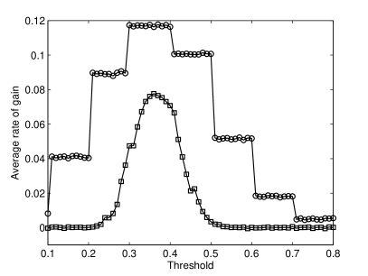
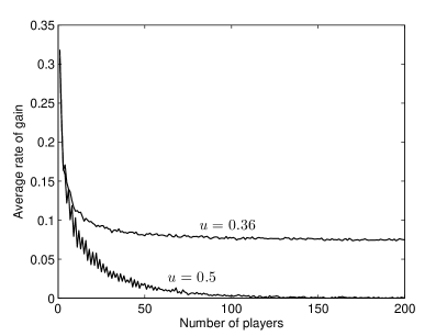
Figure 2: Left: Average rate of gain per player as a function of the threshold, i.e., minimal fraction of votes for A to select this game, for $N=10$ (circles) and $N=100$ (squares) players. Right: Average rate of gain per player as a function of the number of players for two values of the threshold $u$: simple majority, $u=1/2$, and optimal threshold for $N=100$, $u=0.36$.

For finite ensembles the results are very similar. In Fig. 2 (left) we show the average rate of gain per player as a function of the threshold, for $N=10$ and $N=100$ players. We see that the simple majority rule ($u=1/2$) yields a small gain even for $N=10$. On the other hand, a threshold around $u=0.36$ turns out to be optimal for both small ($N=10$) and large ($N=100$) ensembles. Notice however that $u=0.36$ is no longer optimal for infinite ensembles, since gives rise to the stationary periodic sequence ABBABB… For $N=100$, fluctuations are still important (of the order of 10%), and the threshold $u=0.36$ makes a better use of such fluctuations yielding an average gain $g\approx 0.776$ (recall that the average gain with the optimal periodic sequence ABABB… is $g_{opt}\approx 0.07568$). The associated sequence of games is similar to ABBABB… plus some random “mutations” that depend on the random state of the system and improve its overall performance.

Finally, we show in Fig. 2 (right) the average rate of gain per player as a function of the number of individuals in the ensemble for the simple majority threshold ($u=1/2$) and for the optimal threshold found in the cases $N=10$ and $N=100$, namely, $u=0.36$. Both thresholds give similar returns for small ensembles but the simple majority rule rapidly decreases to zero as $N$ increases.

We have to stress that these results are very sensitive to the rules of the games. For instance, the average gain in the case of the short-term optimization vanishes for $N\to\infty$ if the probability to win and loose in each game do not sum up to one, i.e., if there is a non zero probability that players do not change their capitals in each turn [5].

3 Dictatorship

We now consider a model where the choice of the game is made by a single player, the dictator, whereas the rest of the players —the “citizens”— must accept her decision. Hence, the whole ensemble plays game A if the dictator’s capital is a multiple of three and B otherwise. The results of a simulation with 10 players (the dictator plus 9 “citizens”), is shown in Figure 3 (left).

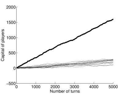
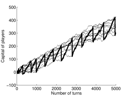
Figure 3: Simulation results for the fixed (left) and alternating (right) dictator model, with 10 players (9 citizens and one dictator). The capital of the dictator at each turn is indicated by the thick line.

This model can be solved analytically, as explained in the Appendix, and the average gain per turn and player for both the dictator and the citizens read, respectively:

$$g_{d} = \frac{12}{37}=0.324...$$

$$g_{c} = \frac{628224}{13685449}=0.0459...$$ (2)

which coincide with those observed in simulations (cfr. Fig. 3, left).

As expected, dictator’s earnings grow fast since she is playing the optimal strategy for a single player. It is not so clear at first sight what will happen to the rest of the players or citizens. Note that the choice of the game does not depend on their capital at all and therefore it should behave exactly as if a given sequence of games was imposed. This sequence is the result of the random walk performed by the dictator’s capital, so it is a random sequence. Interestingly enough, the capital of the citizens increases at a bigger rate than in the optimal random and uncorrelated sequence of games. This optimal random sequence is achieved when games A and B are played at frequencies $\gamma$ and $1-\gamma$, respectively, with $\gamma\approx 0.4146$, and the resulting maximum gain per turn is $g_{max,rand}\approx 0.02620$ [14], significantly smaller than $g_{c}\approx 0.0459$ in Eq. (3). This means that the random sequence of games imposed by the dictator exhibits time correlations which are beneficial for the rest of the players, although the sequence is not correlated with their own state.

The performance of the whole community under the dictator rule is given by the average gain per turn and player:

$$g=\frac{g_{d}+(N-1)g_{c}}{N}$$ (3)

This average gain $g$ is shown in Fig. 4 (solid line). The dictator protocol is better than the democracy with a simple majority rule, but worse than democracy with the optimal threshold. In this protocol, as clearly seen in Fig. 3 (left), the dictator separates from the rest of the players. A similar strategy in ratchets can be useful for segregation of target particles [15].

One could think that the high rate of gain of the dictator will further help to boost the capital of the whole community if the role of the dictator is alternated among all the players. We have explored several versions of this idea. In first place, a purely cyclic dictator among $N$ players yields the same average rate of gain $g$ given by (3), which clearly converges to $g_{c}$ for large $N$. This average rate of gain is the same as in the case of a fixed dictator, although, with a cyclic dictator there is no segregation of a single individual.

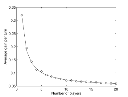
Figure 4: Average gain per turn of the whole community for the fixed or cyclic dictator (solid line, analytical results from Eq. (3)), and for the alternating dictator (circles, simulations over $10^{5}$ turns).

A more elaborated version consists of choosing the poorest individual to play the role of the dictator until she becomes the richest. The result of this protocol is shown in Fig. 3 (right). As in the case of cyclic dictators, the dispersion of capitals is small and all citizens benefit from the strategy, but in this case even those who never become dictators. However, the overall performance of this helping-the-poorest protocol and of the purely cyclic dictator are the same, as shown in Fig. 4. The reason is that Eq. (3) still holds within time intervals where the dictator does not change (see Fig. 3, right), and each of these changes is in fact a relabeling of the players with no effect on the total capital.

These results indicate that Eq. (3) is the optimal gain if we use only the information of the state of one of the players in each turn, although we do not have a rigorous proof of this statement. We will discuss further on this point in Sec. 5.

4 Oligarchy

Since democracy is better for small ensembles, one could try to improve the performance of the whole community allowing a reduced subset of the ensemble, or “oligarchy”, to decide the game to be played. The oligarchs take their decision by voting with a given threshold as in the democratic protocols of Sec. 2.

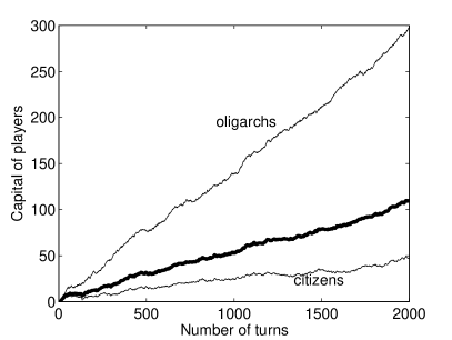
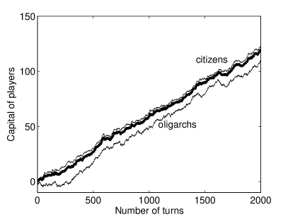
Figure 5: Evolution of the capital in the oligarchy protocol. We plot the average gain per player of 5 oligarchs and 10 citizens, with threshold $5/13$. Left: fixed oligarchy. Right: adaptive oligarchy, formed by the 5 poorest players in each turn.

Figure 5 (left) presents a typical realization of the game with 5 oligarchs and 10 citizens. The oligarchs use a short-term optimization with threshold $u=5/13$. Only the average rate of gain for oligarchs and citizens are shown, for clarity. The capital of the oligarchy behaves exactly as in the democracy case with only 5 players. As in the dictatorship, the capital of the rest of the citizens also increases at a larger rate than in any random combination of games.

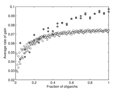
Figure 6: Rate of gain per player in the oligarchy protocol as a function of the fraction of oligarchs with threshold $u=0.36$: fixed oligarchy (circles) and adaptive (squares); for $N=20$ (grey symbols) and $N=100$ (white symbols).

As we have seen in section 2, the rate of gain of a set of players taking a democratic decision decreases with the number of players. Consequently, one could ask if there exists an optimal size for the oligarchy. Our simulations, shown in Fig. 6, indicate that this optimal oligarchy is the whole ensemble of players. The reason is that increasing the size of the oligarchy has two effects: a) the oligarchs’ weight in the total average increases and b) the sequence of games is closer to ABB (or ABABB, depending on the threshold) which is sound for everybody.

Again, one could try to improve the average returns by allowing the poorest players to choose the game. With this idea in mind, we have analyzed a special case of adaptive oligarchy: in each turn, the oligarchy is formed by the $n_{olig}$ poorest players. The results are shown in both Figs. 5 and 6. As in the case of the alternating dictator, giving the role of oligarchs to the poorest players has the only effect of keeping closer all individuals in the ensemble, but does not affect the total capital: Fig. 6 shows that the total capital of the ensemble in the fixed or adaptive oligarchy are very similar, both for small ($N=20$) and large ($N=100$) ensembles. In this latter case, the result was expected, since for large oligarchies, no matter if they are fixed or not, the sequence of games is close to ABBABB… plus some small fluctuations beneficial only for the oligarchs, but not affecting the rest of players.

5 Conclusions

We have studied several strategies for a collective decision making in ensembles of individuals playing paradoxical games against the casino.

The optimal “blind” choice of games is the periodic sequence ABABBABABB… For small ensembles a democratic choice with a threshold around 0.36 for selecting game A can do better than the optimal “blind” sequence of games, even up to $N=100$ players. However, this is expected since, for this size, fluctuations are of the order of 10%, big enough to be used by strategies depending on the actual state of the system.

The present study prompts several questions about how fluctuations can be used to improve the performance of the ensemble. Firstly, our results with dictators and oligarchies indicate that the gain that can be achieved depends more on the information used in each strategy than on its details. For instance, our simulations show that adaptive and fixed dictators yield the same gain per player. Oligarchies exhibit a similar feature. Secondly, in the case of oligarchy, we have found that it is always better the decision taken by the whole ensemble (at least for certain thresholds close to the optimal one) than by any subset. That is, it is better to use the maximum information available.

It is worth to mention that the actual optimal strategies for $N$ finite are based on the complete state of the system, i.e., on the vector (1) [16, 17], whereas the only information that we have used here is the fraction $\pi_{0}(t)$ of players in the bad coin of game B. However, the analysis could be extended to incorporate this additional information without affecting our main conclusions.

Touchette and Lloyd [18] have explored the limitations that thermodynamics imposes to the energetics of some controlled physical systems, based on the information used in the feedback control. In this paper we have shown that analogous limitations apply to the gain of players or, equivalently, to the velocity of random walkers in non-homogeneous and asymmetric media. We believe that our results could be explained and generalized by a theoretical framework that relates the measure of the information used in a control protocol with the performance of such a protocol in stochastic systems with feedback, following similar lines as those in Ref. [18].

6 Analytical solution of the fixed-dictator protocol

Let $X_{d}(t)$ and $X(t)$ be the capital of the dictator and of a given citizen at time $t$, respectively. We define the vector ${\bf Y}(t)$ as:

$${\textbf{Y}}(t)=\left(\begin{array}[]{cc}X_{d}(t)\ \textrm{mod}\ 3\\ X(t)\ \textrm{mod}\ 3\end{array}\right)$$ (4)

which can take on nine different values: (00), (01), (02), (10), (11), (12), (20), (21, (22). The vector ${\bf Y}(t)$ is a Markov chain with the following transition matrix (we number the nine states in the same order as in the previous list):

$$\Pi=\left(\begin{array}[]{ccccccccc}0&0&0&0&\frac{1}{16}&\frac{3}{16}&0&\frac{3}{16}&\frac{9}{16}\\ 0&0&0&\frac{1}{40}&0&\frac{1}{16}&\frac{3}{40}&0&\frac{3}{16}\\ 0&0&0&\frac{9}{40}&\frac{3}{16}&0&\frac{27}{40}&\frac{9}{16}&0\\ 0&\frac{1}{4}&\frac{1}{4}&0&0&0&0&\frac{1}{16}&\frac{3}{16}\\ \frac{1}{4}&0&\frac{1}{4}&0&0&0&\frac{1}{40}&0&\frac{1}{16}\\ \frac{1}{4}&\frac{1}{4}&0&0&0&0&\frac{9}{40}&\frac{3}{16}&0\\ 0&\frac{1}{4}&\frac{1}{4}&0&\frac{3}{16}&\frac{9}{16}&0&0&0\\ \frac{1}{4}&0&\frac{1}{4}&\frac{3}{40}&0&\frac{3}{16}&0&0&0\\ \frac{1}{4}&\frac{1}{4}&0&\frac{27}{40}&\frac{9}{16}&0&0&0&0\end{array}\right)$$ (5)

Each entry of the matrix is the transition probability from a state to another, and can be derived directly from the rules of the game. For instance, the transition probability from (01) to (12) is $p_{a}(1-p_{a})=1/4$, since the dictator in the initial state has a capital multiple of three and chooses A as the game to be played. This corresponds to $\Pi_{6,2}$. The transition probability from (21) to (02) is $p_{b2}p_{b1}=9/16$, since in this transition both the dictator and the citizen win playing game B. Therefore $\Pi_{3,8}=9/16$.

The matrix $\Pi$ is an stochastic matrix with one eigenvalue equal to 1. The corresponding eigenvector, after normalization, is the stationary probability distribution of the Markov chain and reads:

$$P_{st}=\frac{\left(1759355,633035,2416011,1246210,1218764,1233796,1684790,1368644,2124844\right)}{13685449}$$ (6)

From this distribution one can calculate the winning probabilities for the dictator and the citizens, taking into account the winning probability in each state. For instance, for the dictator we have:

$$P_{win,dict}=(P_{st,1}+P_{st,2}+P_{st,3})p_{a}+(P_{st,4}+P_{st,5}+P_{st,6}+P_{st,7}+P_{st,8}+P_{st,9})p_{b1}$$ (7)

since the dictator wins with probability $p_{a}$ in the three first states and with probability $p_{b1}$ in the other six states.

Finally, the average rate of gain per player and per turn is, respectively:

$$g_{d} = \lim_{t\to\infty}\frac{X_{d}(t)}{t}=2P_{win,dict}-1=\frac{12}{37}=0.324...$$

$$g_{c} = \lim_{t\to\infty}\frac{X(t)}{t}=2P_{win,cit}-1=\frac{628224}{13685449}=0.0459...$$ (8)

These values coincide with the results of the simulations for $\epsilon=0$.

References

- [1] S. Nitzan and J. Paroush, Collective decision making : an economic outlook (Cambridge University Press, Cambridge, 1985).
- [2] G.P. Harmer and D. Abbott, Nature 402, 864 (1999).
- [3] J.M.R. Parrondo and L. Dinis, Cont. Phys. 45, 147 (2004).
- [4] L. Dinis and J.M.R. Parrondo, Physica A 343, 701 (2004).
- [5] L. Dinis and J.M.R. Parrondo, Europhys. Lett. 63, 319 (2003).
- [6] A.P. Flitney, J. Ng, and D. Abbott, Physica A 314, 35 (2002).
- [7] C.F. Lee, N.F. Johnson, F. Rodriguez, and L. Quiroga, Fluct. and Noise Lett. 2, L293 (2002).
- [8] J. Buceta, C. Escudero, F.J. de la Rubia, and K. Lindenberg, Phys. Rev. E 69, 021906 (2004).
- [9] D.M. Wolf, V.V. Vazirani, and A.P. Arkin. J. Theor. Biol. 234, 227 (2005).
- [10] J.S. Canovas, A. Linero, and D. Peralta-Salas, Physica D 218, 177 (2006).
- [11] F.J. Cao, L. Dinis, and J.M.R. Parrondo, Phys. Rev. Lett. 93, 040603 (2004).
- [12] L. Dinis, J.M.R. Parrondo, and F.J. Cao, Europhys. Lett. 71, 536 (2005).
- [13] R. Iyengar and R. Kohli, Complexity 9, 23 (2003).
- [14] G.P. Harmer, D. Abbott, P.G. Taylor, and J.M.R. Parrondo, Chaos 11 705 (2001).
- [15] H. Linke. To be published.
- [16] B. Cleuren, Ph.D. thesis, University of Hasselt, 2004.
- [17] L. Dinis, Ph.D. thesis, Universidad Complutense de Madrid, 2005.
- [18] H. Touchette and S. Lloyd, Phys. Rev. Lett. 84, 1156 (2000).