Clustering of $\gamma$-ray selected 2LAC Fermi Blazars

Abstract

We present the first measurement of the projected correlation function of 485 $\gamma$-ray selected Blazars, divided in 175 BLLacertae (BL Lacs) and 310 Flat Spectrum Radio Quasars (FSRQs) detected in the 2-year all-sky survey by Fermi-Large Area Telescope. We find that Fermi BL Lacs and FSRQs reside in massive dark matter halos (DMHs) with logM_h=13.35${}^{+0.20}_{-0.14}$ and logM_h = 13.40${}^{+0.15}_{-0.19}$ h^-1 M_⊙, respectively, at low (z $\sim$ 0.4) and high (z $\sim$ 1.2) redshift. In terms of clustering properties, these results suggest that BL Lacs and FSRQs are similar objects residing in the same dense environment typical of galaxy groups, despite their different spectral energy distribution, power and accretion rate. We find no difference in the typical bias and hosting halo mass between Fermi Blazars and radio-loud AGNs, supporting the unification scheme simply equating radio-loud objects with misaligned Blazar counterparts. This similarity in terms of typical environment they preferentially live in, suggests that Blazars preferentially occupy the centre of DMHs, as already pointed out for radio-loud AGNs. This implies, in light of several projects looking for the $\gamma$-ray emission from DM annihilation in galaxy clusters, a strong contamination from Blazars to the expected signal from DM annihilation.

1. Introduction

Blazars are radio-loud Active Galactic Nuclei (AGNs) with jets pointing at us rather than in the plane of the sky (Blandford et al. 1978, Urry & Padovani 1995 and references therein). They are characterized by the luminous, rapidly variable and polarized non-thermal continuum emission, extending from radio to $\gamma$-ray (GeV and TeV) energies. They emit most of their electromagnetic output in the $\gamma$-ray band and they are the most numerous class of extragalactic objects detected by the Large Area Telescope (LAT) onboard the Fermi satellite (Nolan et al. 2012) and by ground-based Cherenkov telescopes (see Hinton et al. 2009 for a review). The overall spectral energy distribution (SED) of low power Blazars is characterized by two broad distinctive humps peaking in the UV-soft X-ray band (due to synchrotron emission of relativistic electrons) and in the GeV-TeV band (due to inverse Compton scattering of soft photons by the same relativistic electrons). High power Blazars peak at smaller frequencies (sub-mm and $\sim$MeV).

Blazars are usually separated into low power BL Lacertaes (BL Lacs) and high power flat-spectrum radio quasars (FSRQs). BL Lacs are typically completely dominated by the jet emission, emitting a double humped synchrotron self-Compton spectrum. The FSRQs are more complex, showing clear signatures of a ‘normal’ AGN disc and broad line region (BLR), unlike the BL Lacs which generally show no broad lines or disc emission. Thus the nature of the accretion flow itself is different in BL Lacs and FSRQs, with the latter showing a standard disc which is absent from the former. This can be linked to the clear distinction in Eddington ratio between BL Lacs and FSRQs, with the BL Lacs all consistent with ṁ = Ṁ/Ṁ${}_{Edd}<0.01$ (where $\eta$Ṁ_Eddc² = L_Edd and the efficiency $\eta$ depends on BH spin) while the FSRQs have ṁ $>$ 0.01 (see e.g. Ghisellini et al. 2010, 2013). According to unified schemes, Blazars are misaligned counterparts of radio galaxies, with FSRQs made by powerful Fanaroff-Riley type 2 (FRII) radio-galaxies and BL Lacs related to low power FRI radio galaxies.

As shown in Ackermann et al. (2011), the Fermi $\gamma$-ray Space Telescope provided one of the largest sample of Blazars up to z=3.1, allowing for the first time the study of the spatial distribution of $\gamma$-ray selected AGN in the Universe. AGN clustering measurements are powerful in providing information about the physics of galaxy/AGN formation and evolution, the typical environment that AGN preferentially live in and to put constraints on the mechanisms that trigger the AGN activity. Up to now a large amount of research in the field of clustering has been performed in optical, radio and X-ray band. The amplitude of the quasar correlation function suggests that optically selected quasars are hosted by halos of roughly constant mass, a few times 10¹² M_⊙ h^-1, out to z$\sim$3-4 (e.g., Croom et al. 2005, Porciani & Norberg 2006, Myers et al. 2007, Ross et al. 2009, da Angela et al. 2008). On the other hand, measurements of the spatial distribution of X-ray AGN show that they are located in galaxy group-sized DMHs with M_h = 10^13-13.5 M_⊙ h^-1 at low ($\sim$0.1) and high ($\sim$1) redshift (see Cappelluti, Allevato & Finoguenov 2012 for a review). The fact that DMH masses of this class of moderate luminosity AGN is estimated to be, on average, larger than those of luminous quasars, has been interpreted as evidence against cold gas accretion via major mergers in those systems (e.g. Allevato et al. 2011; Mountrichas & Georgakakis 2012), and/or as support for multiple modes of BH accretion (cold versus hot accretion mode, Fanidakis et al. 2013).

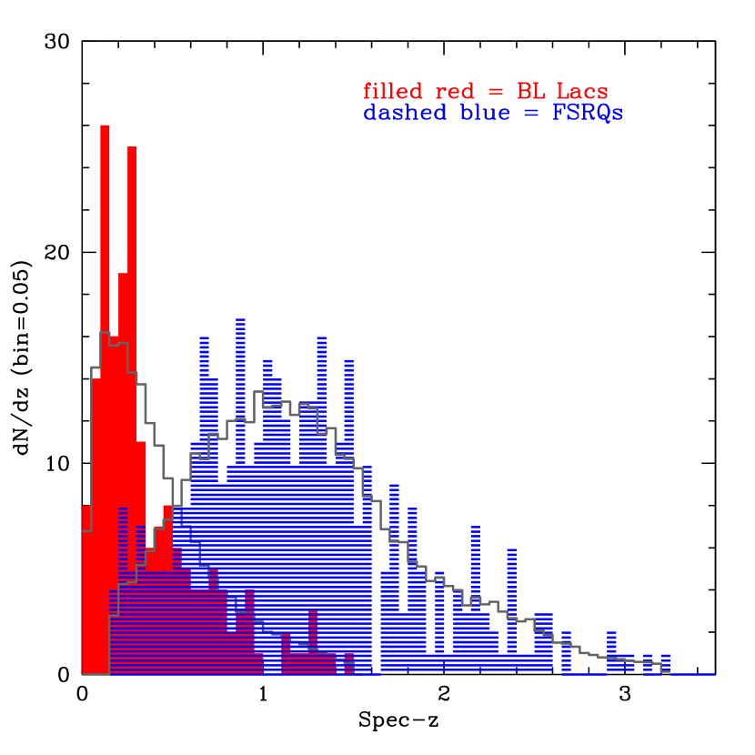
Figure 1.— Redshift distribution of 175 2LAC BL Lacs (filled red histogram), 310 2LAC FSRQs (dashed blue histogram) and of the corresponding random sources (grey empty histograms), where the random redshifts have been obtained using a Gaussian smoothing with $\sigma$=0.2.

Compared to X-ray and optically-selected sources, radio-selected AGN are more likely found in group/cluster environments (Smolcic et al. 2011) and are mainly hosted by massive early-type galaxies (e.g. Smolcic et al. 2008, 2009). This result is also confirmed by clustering studies showing that radio AGNs have the same clustering amplitude of local elliptical galaxies (e.g., Magliocchetti et al. 2004, Mandelbaum et al. 2009; Wake et al. 2008, Hickox et al. 2009), with a strong dependence on radio luminosity (e.g., Overzier et al. 2003). Magliocchetti et al. (2004) found that faint radio-FIRST AGNs reside in DMHs more massive than 13.4 M_⊙, which corresponds (following Ferrare 2002) to a threshold BH mass of $\sim$ 10⁹ M_⊙. This minimum mass required to have radio-AGNs is larger than that obtained for radio-quiet quasars in the same redshift range. Moreover, Hickox at al. (2009) found that radio AGNs reside in DMHs with M_h = 3 $\times$ 10¹³ h^-1 M_⊙, while Mandelbaum et al. (2009) estimated a mass (deduced from g-g lensing) of 1.6 $\times$ 10¹³ h^-1 M_⊙ for SDSS radio AGNs. The radio luminosities of these radio AGNs range from 10²³ to 10²⁶ W Hz^-1, i.e. they are mainly FRI systems.

The clustering signal of radio-loud FRI AGNs has been also modelled by using the halo occupation distribution (HOD). Wake et al. (2008) showed that 2SLAQ radio AGNs at 0.4 $<$ z $<$ 0.7, preferentially occupy central galaxies respect to satellites. This HOD has been directly confirmed by Smolcic et al. (2011), who also found that low-power radio COSMOS AGNs are preferentially associated with galaxies close to the centre ($<$0.2$R_{200}$).

Clustering of $\gamma$-ray emitting AGN has never been studied and Fermi is the only instrument capable to perform such an analysis. Following the argument that Blazars are simply mislagned counterpart of radio galaxies, we expect that $\gamma$-ray selected Blazars behave similarly to radio-AGN, i.e. we expect that they are hosted by the most massive DMH halos at each epoch, with mass greater than few times 10¹³ M_⊙.

Throughout this work we will assume a $\Lambda$CDM cosmology, with $\Omega_{M}$ = 0.3, $\Omega_{\Lambda}$ = 0.7, $\Omega_{b}$= 0.045, $\sigma_{8}$ = 0.8. All distances are comoving and quoted in units of Mpc h^-1, assuming h = $H_{0}$/100 km s^-1. The symbol log indicates a base-10 logarithm.

Table 12LAC Fermi AGN Samples

(1)	(2)	(3)	(4)	(5)	(6)	(7)	(8)	(9)	(10)
Sample	N	$\langle z\rangle$	$r_{0}$	$\gamma$	$r_{0,\gamma=1.8}$	$b_{PL}$	$b$	$\frac{\chi_{min}^{2}}{d.o.f.}$	logMh
			Mpc h-1		Mpc h-1	$\sigma_{8,AGN}(z)/\sigma_{DM}(z)$	Halo Model		h-1M⊙
BL Lac	175	0.38	6.90${}^{+0.34}_{-1.46}$	1.64${}^{+0.35}_{-0.30}$	7.88$\pm 0.66$	1.52$\pm 0.21$	1.84$\pm 0.25$	6.3/8	13.35${}^{+0.20}_{-0.14}$
FSRQ	310	1.18	7.7${}^{+3.8}_{-3.1}$	1.5${}^{+0.3}_{-0.4}$	11.2$\pm 1.2$	3.0$\pm$0.3	3.30$\pm 0.41$	22.3/8	13.40${}^{+0.15}_{-0.19}$

Note. — Values of $r_{0}$, $\gamma$ and $r_{0,\gamma=1.8}$ are obtained from a power-law fit of the 2PCF over the range $r_{p}$=1-80 Mpc h^-1, using the full error covariance matrix and minimizing the correlated $\chi^{2}$ values. The bias parameters, $b_{PL}=\sigma_{8,AGN}(z)/\sigma_{DM}(z)$, are based on the power-law best fit parameters $r_{0,\gamma=1.8}$ and the uncertainties are derived from the standard deviation of $\sigma_{8,AGN}(z)$, where the 1$\sigma$ errors on $\sigma_{8,AGN}(z)$ correspond to $\chi^{2}=\chi_{min}^{2}+1$. The bias factors in col (8) are estimated using the halo model, $w_{mod}(r_{p})=b^{2}w_{DM}(r_{p},z)$ where $w_{DM}(r_{p},z)$ is the dark matter 2PCF at large scale (2-halo term) evaluated at the mean redshift of the samples. The 1$\sigma$ errors on the bias correspond to $\chi^{2}=\chi^{2}_{min}+1$ where the $\chi_{min}^{2}$ is given in col (9). The correlations between errors have been taken into account through the inverse of the covariance matrix. To derive logM_h we followed the bias-mass relation b(M_h,z) described in van den Bosch (2002) and Sheth et al. (2001), using the bias factors in col (8).

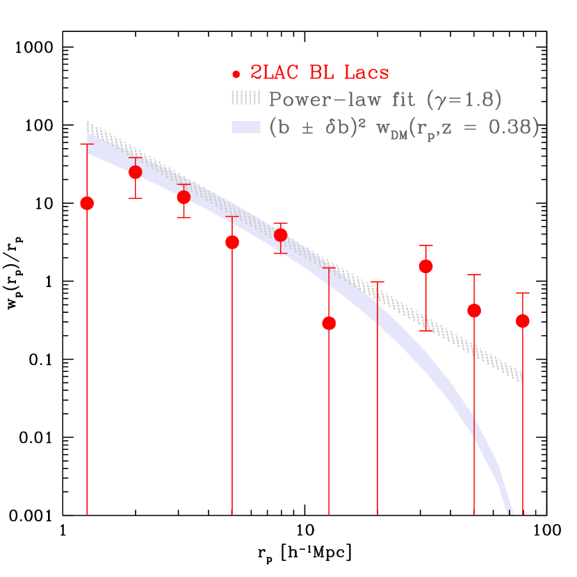
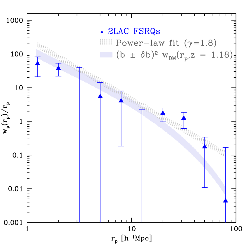
Figure 2.— Projected 2PCF of 175 2LAC BLLacs (red circles) and 310 FSRQs (blue triangles) compared to $(b\pm\delta b)^{2}w_{DM}(r_{p})$ (blue shaded region), where $(b\pm\delta b)^{2}$ is the square of the bias factor $\pm 1\sigma$ (Table 1, col 8) and $w_{DM}(r_{p})$ is the dark matter 2-halo term evaluated at the mean redshift of the sample. For comparison, the dotted grey regions mark the best-fit power-laws with $\gamma=1.8$ and $r_{0}$ given in Table 1, col 6.

2. AGN Catalog

The second catalog of AGNs (2LAC) detected by Fermi- Large Area Telescope (LAT) in two years of scientific operation has been presented in Ackermann et al. (2011). The entire sample includes 1017 $\gamma$-ray sources. For each source they found a counterpart comparing the sample with known source catalogs and with uniform surveys in the radio and X-ray bands. The associations have been done with statistical approaches such as Bayesian, likelihood ratio and logN-logS association methods (see Ackermann et al. 2011 for more details). The 1017 LAT sources have been classified in FSRQ, BL Lac object, radio galaxy, steep-spectrum radio quasar (SSRQ), Seyfert, narrow line Seyfert 1, starburst galaxy. The ingredients of the classification are optical spectra or other Blazar characteristics (radio loudness, broadband emission, variability and polarization) and the synchrotron-peak frequency of the broadband SED. All the sources without a good optical spectrum or without an optical spectrum at all are defined as AGU and AGNs. All the objects with single counterparts and without analysis flag (886/1017) define the Clean Sample, which comprises 395 BL Lacs and 310 FSRQs, 157 sources of unknown type, 22 other AGNs and 2 starburst galaxies. We focus our analysis on objects classified as Blazars, i.e. BL Lacs and FSRQs, with known spectroscopic redshift. Unfortunately only 46% of BLLacs (175/395) have measured redshifts which extend to z=1.5. Otherwise the redshift distribution of FSRQs (310) peaks around z=1 and extends to z=3.10. The redshift distributions of 175 2LAC BL Lacs and 310 2LAC FSRQs are compared in Fig. 1. The mean redshift is $\langle z\rangle$=0.38 and 1.18 for BL Lacs and FSRQs, respectively.

3. 2-point correlation function

The two-point correlation function (2PCF) $\xi(r)$ is defined as the excess probability $dP$ above a Poisson distribution of finding an object in a volume element $dV$ at a distance $r$ from another randomly chosen object (Peebles 1980). With a redshift survey, we cannot directly measure $\xi(r)$ in physical space because peculiar motions of galaxies distort the line-of-sight distances inferred from redshift. To separate the effects of redshift distortions, the 2PCF is measured in two dimensions, $r_{p}$ and $\pi$ which are the projected comoving separations between AGN pairs in the directions perpendicular and parallel to the line-of-sight, respectively. Following Davis & Peebles (1983) $r_{p}$ and $\pi$ are defined as:

$$\pi = \frac{\textbf{s}\cdot\textbf{l}}{|\textbf{l}|}$$ (1)

$$r_{p} = \sqrt{(\textbf{s}\cdot\textbf{s}-\pi^{2})}$$ (2)

where $r_{1}$ and $r_{2}$ are the redshift positions of a pair of AGN, $s$ is the redshift-space separation $(r_{1}-r_{2})$ and $l=(r_{1}+r_{2})/2$ is the mean distance to the pair. We then measure the 2PCF on a two-dimensional grid of separations r_p and $\pi$, obtaining the projected correlation function w_p(r_p) defined by Davis & Peebles (1983) as:

$$w_{AGN}(r_{p})=2\int_{0}^{\pi_{max}}\xi(r_{p},\pi)d\pi$$ (3)

Usually $\xi(r_{p},\pi)$ is measured using the estimator defined in Landy & Szalay (1993, LS):

$$\xi=\frac{1}{RR}[DD-2DR+RR]$$ (4)

The LS estimator is then defined as the ratio between AGN pairs in the data sample and pairs of sources in the random catalog, as a function of the projected comoving separations between the objects. This estimator has been used to measure the 2PCF of X-ray, optically and radio selected AGN (e.g. Zehavi et al. 2005, Li et al. 2006, Coil et al. 2009, Hickox et al. 2009, Gilli et al. 2009, Allevato et al. 2011).

The choice of $\pi_{max}$ is a compromise between having an optimal signal-to-noise ratio and reducing the excess noise from high separations. Usually, the optimum $\pi_{max}$ value can be determined by estimating $w_{p}(r_{p})$ for different values of $\pi_{max}$ and finding the value at which the 2PCF levels off. Following this approach, we fixed $\pi_{max}$ = 40 h^-1Mpc in the following analysis which ensures the $w_{p}(r_{p})$ convergence.

The measurement of the 2PCF required the construction of an AGN random catalog with the same selection criteria and observational effects as the data. This random sample serve as an unclustered distribution to which to compare the data. We separately created a random catalog for BLLacs and FSRQs, reproducing the space and flux distributions of 2LAC Blazars. In detail, the random sources are randomly placed in the sky and the fluxes randomly drawn from the catalog of real fluxes and kept in the random sample if above the values of the sensitivity map (published by Abdo et al. 2010) at those random positions. We prefer this method with respect to the one that keeps the angular coordinates unchanged and then has the disadvantage of removing the contribution to the signal due to angular clustering. The redshifts are randomly extracted from a smoothed redshift distribution of the real sources. Specifically, we assume a Gaussian smoothing length $\sigma_{z}=0.2$. This is a good compromise between scales that are too small, which would suffer from local density variations, and those that are too large, which would oversmooth the distribution. However, we verified that our results do not change significantly using $\sigma_{z}$ = 0.2-0.4. Fig 1 compares the redshift distribution of 175 BL Lacs (in red) and 310 FSRQs (in blue) with the redshift distribution of the random sources, where the random redshifts have been obtained using a Gaussian smoothing with $\sigma$=0.2.

Since adjacent bins in w${}_{p}(r_{p})$ are correlated, as are their errors, we constructed the covariance matrix M_i,j (Miyaji et al. 2007), which reflects the degree to which bin $i$ is correlated with bin $j$. The covariance matrix is used to obtain reliable fits to w_p(r_p) by minimizing the correlated $\chi^{2}$ values. By using a bootstrap resampling technique (Coil et al. 2009; Hickox et al. 2009; Krumpe et al. 2010; Cappelluti et al. 2010), we estimated the covariance matrix as:

$$M_{i,j} = \frac{1}{N_{boot}}\sum_{k=1}^{N_{boot}}\left(w_{k}(r_{p,i})-\langle w(r_{p,i})\rangle\right)$$ (5)

$$\times \left(w_{k}(r_{p,j})-\langle w(r_{p,j})\rangle\right)$$ (6)

We calculate w_p(r_p) N_boot = 100 times and $w_{k}(r_{p,i})$ and $w_{k}(r_{p,j})$ are from the k-th bootstrap. $\langle w(r_{p,i})\rangle$ and $\langle w(r_{p,j})\rangle$ are the averages over all the bootstrap samples.

In the halo model approach, the 2PCF is modelled as the sum of contributions from AGN pairs within individual DMHs (1-halo term, $r_{p}\lesssim 1$ Mpc h^-1) and in different DMHs (2-halo term, $r_{p}\gtrsim 1$ Mpc h^-1). The superposition of both the terms describes the shape of the 2PCF better than a simple power-law. In this context, the bias parameter $b$ reflects the amplitude of the AGN large-scale clustering (2-halo term) relative to the underlying DM distribution, i.e.:

$$w_{mod}(r_{p})=b^{2}w_{DM}^{2-h}(r_{p},z)$$ (7)

The DM 2-halo term is measured at the mean redshift of the sample, using:

$$w_{DM}^{2-h}(r_{p})=r_{p}\int_{r_{p}}^{\infty}\frac{\xi^{2-h}_{DM}(r)rdr}{\sqrt{r^{2}-r_{p}^{2}}}$$ (8)

where

$$\xi^{2-h}_{DM}(r)=\frac{1}{2\pi^{2}}\int P^{2-h}(k)k^{2}\left[\frac{sin(kr)}{kr}\right]dk$$ (9)

$P^{2-h}(k)$ is the linear power spectrum (Efstathiou, Bond & White 1992), assuming a power spectrum shape parameter $\Gamma=0.2$ which corresponds to $h=0.7$ (see Seljak 2000, Hamana et al. 2002).

4. Results

The projected 2PCFs of 2LAC BL Lacs and FSRQs are shown in Fig. 2 in the range $r_{p}$=1-80 h^-1 Mpc. The 1$\sigma$ errors on $w_{p}(r_{p})$ are the square root of the diagonal components of the covariance matrix. We find a significant signal at almost all the sampled scales for both BL Lacs and FSRQs, even if with relatively large uncertainty due to the small number of AGN pairs at each separation. On the contrary, we observe a lack of AGN pairs at smaller separation ($r_{p}\lesssim 1$ Mpc h^-1).

We derive the best-fit bias for 2LAC Blazars by using a $\chi^{2}$ minimization technique with 1 free parameter, where $\chi^{2}=\Delta^{T}M^{-1}_{cov}\Delta$. In detail, $\Delta$ is a vector composed of $w_{AGN}(r_{p})-w_{mod}(r_{p})$ (see Eq. 3 and 7), $\Delta^{T}$ its transpose and M_cov is the covariance matrix. The dark matter 2PCF, as defined in Eq. 8, is evaluated at the mean redshift of the samples, i.e. $\langle z\rangle$=0.38 and $\langle z\rangle$=1.18 for BL Lacs and FSRQs, respectively. For BL Lacs we find a linear bias of 1.84$\pm 0.25$ at $\langle z\rangle$=0.38 while for FSRQs we obtained b=3.30$\pm 0.41$ at $\langle z\rangle$=1.18 (see Table 1). The errors correspond to $\Delta\chi^{2}$ = 1.

For comparison, we also fit the 2PCF with a power-law model of the form $w_{p}(r_{p})=(r_{0}/r_{p})^{-\gamma}(\Gamma(1/2)\Gamma[(\gamma-1)/2])/(\Gamma(\gamma/2))$ (Coil et al. 2009, Hickox et al. 2009, Gilli et al. 2009, Krumpe et al. 2010,2012, Cappelluti et al. 2010), using a $\chi^{2}$ minimization technique, with $\gamma$ and $r_{0}$ as free parameters. As shown in Table 1, we derive $\gamma$=1.64${}^{+0.35}_{-0.30}$, r₀=6.90${}^{+0.34}_{-1.46}$ Mpc h^-1 for BL Lacs and $\gamma$=1.5${}^{+0.3}_{-0.4}$, r₀=7.7${}^{+3.8}_{-3.1}$ Mpc h^-1 for FSRQs. The best-fit values of the power-law slope are consistent with several results on the clustering of X-ray selected AGNs (e.g. Coil et al. 2009, Krumpe et al. 2010, Cappelluti et al. 2010) and optically selected 2QZ luminous quasars (Porciani et al. 2004). On the other hand, we argue that the low power-law slope observed for 2LAC Blazars might be due to the lack of clustering signal at small scale ($r_{p}\lesssim 1$ Mpc h^-1).

Finally, fixing $\gamma$ = 1.8, we find that BL Lacs at $\langle z\rangle\sim$0.4 have a correlation length of $r_{0}$=7.88$\pm 0.66$ Mpc h^-1 while FSRQs at $\langle z\rangle\sim$1.2, have a larger correlation length of $r_{0}$=11.2$\pm 1.2$ Mpc h^-1. At similar redshift ($z\sim 1.4$), Shanks et al. (2011) derived a lower best-fit r₀ = 5.90 $\pm$ 0.14 Mpc h^-1 (and $\gamma$=1.8) for quasars in SDSS DR5, 2SLAQ and 2QZ surveys.

The power-law best-fit parameters are related to $\sigma_{8,AGN}(z)$, i.e. the rms fluctuations within a sphere with a co-moving radius of 8 h^-1Mpc (Peebles 1980):

$$(\sigma_{8,AGN})^{2}=J_{2}(\gamma)(\frac{r_{0}}{8Mpc/h})^{\gamma}$$ (10)

where $J_{2}(\gamma)=72/[(3-\gamma)(4-\gamma)(6-\gamma)2^{\gamma}]$. Following this argument, we further derive the bias $b_{PL}=\sigma_{8,AGN}(z)/\sigma_{DM}(z)$ where $\sigma_{DM}(z)$ is evaluated at 8 Mpc h^-1 and normalized to a value of $\sigma_{DM}(z=0)=0.8$. As shown in Table 1, fixing the power-law slope $\gamma$=1.8, we find a bias factor for 2LAC BL Lacs and FSRQs quite consistent with the values derived using the halo model approach. The uncertainties on the bias factors are derived from the 1$\sigma$ errors on $\sigma_{8,AGN}(z)$, which correspond to $\chi^{2}=\chi^{2}_{min}+1$.

The projected 2PCF is always obtained by integrating out to some finite $\pi_{max}$ rather than to infinity. Van den Bosch 2013 demonstrates that this finite integration range introduces errors on the largest scales probed by the data ($\sim$20 h^-1Mpc). This is due to the fact that the Kaiser effect (coherent galaxy motion that causes an apparent contraction of structure along the line of sight in redshift space, Kaiser 1987) can not be ignored on scales $>\pi_{max}$. In order to estimate the error introduced in our 2PCF measurements by the finite integration range, we use the correction factor derived in Van den Bosch 2013 (see Equation 48 and Figure 6 therein) for $\pi_{max}$=40 h^-1Mpc and by integrating over all halo masses.

We find that, without the correction, we underestimate the projected 2PCF by $\sim$35% at r_p=20 h^-1Mpc for both 2LAC BL Lacs and FSRQs. However this error only slightly affects the bias factors. (col 8 Table 1). In fact, by introducing the correction factor the bias factors of BL Lacs and FSRQs (based on power-law best fit parameters or halo model) increase by $\sim$6%, i.e. within the statistical error of $\sim$14%. In agreement with Van den Bosch 2013, the result suggests that this effect is important when using projected correlation functions to constrain cosmological parameters. However, it only introduces a small change in the bias of relatively small AGN samples.

Finally, we use the bias factor to estimate the typical DMH mass hosting the different Blazar samples (under the assumption that the bias only depends on the halo mass). To this end, we followed the bias-mass relation $b(M_{h},z)$ defined by the ellipsoidal collapse model of Sheth et al. (2001) and the analytical approximation of van den Bosch (2002). Table 1 shows the typical DMH mass of 2LAC Blazars derived by using the bias as defined in the halo model (col 8). We found that BL Lacs and FSRQs reside in massive DM halos with logM_h=13.35${}^{+0.20}_{-0.32}$ and logM_h=13.40${}^{+0.15}_{-0.25}$ h^-1M_⊙, respectively. These results infer for the first time that $\gamma$-ray selected AGN reside in group-sized halos at low ($\sim$0.4) and at high ($\sim$1.2) redshift.

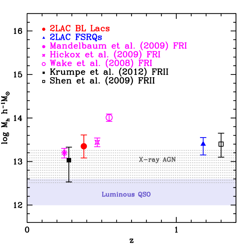
Figure 3.— Typical DMH mass of 2LAC BL Lacs at $\langle z\rangle$=0.38 (red circle) and 2LAC FSRQs at $\langle z\rangle$=1.18 (blue triangle), estimated following the bias-mass relation b(M_h,z) described in van den Bosch (2002) and Sheth et al. (2001). The magenta data points mark the halo mass of radio-loud FRI objects from SDSS (Mandelbaum et al. 2009, deduced from g-g lensing), AGES (Hickox et al. 2009, derived using the bias-mass relation b(M_h,z) of Shen et al. 2001) and 2SLAQ LRG survey (Wake et al. 2008, based on the halo occupation distribution). The black data points show the halo mass of radio loud broad line SDSS quasars as estimated in Krumpe et al. (2012) and Shen et al. (2009) derived using the bias-mass relation of Sheth et al. (2001). The quoted typical DMH masses are scaled to the same cosmology ($\Omega_{M}=0.3$, $\Omega_{\Lambda}=0.7$ and $\sigma_{8}=0.8$). The halo mass evolution with redshift is shown for comparison for optically selected quasars (shaded region, Croom et al. 2005, Porciani et al. 2004, Myers et al. 2006, Shen et al. 2009, Ross et al. 2009, da Angela et al. 2008), and X-ray selected AGN (dotted shaded region, Cappelluti et al. 2010, Allevato et al. 2011, Krumpe et al. 2010, 2012, Hickox et al. 2009, Mountricas et al. 2013, Koutoulidis et al. 2012).

5. Discussion and conclusions

We have used a sample of 485 $\gamma$-ray selected 2LAC Blazars (175 BL Lacs and 310 FSRQs) detected in the 2-year all-sky survey of the Fermi satellite, to measure the clustering amplitude and to estimate characteristic DM halo masses. We find that BL Lacs and FSRQs inhabit massive DMHs with logM_h=13.35${}^{+0.20}_{-0.14}$ and logM_h = 13.40${}^{+0.15}_{-0.19}$ h^-1 M_⊙, respectively, at low (z $\sim$ 0.4) and high (z $\sim$ 1.2) redshift. Usually, BL Lacs and FSRQs have different power, SED and Eddington ratio. In detail, low power BL Lacs are consistent with ṁ $<0.01$, while high power FSRQs have accretion rates above this value (see e.g. Ghisellini et al. 2010, 2013). In terms of clustering properties, our results suggest that BL Lacs and FSRQs are similar objects preferentially residing in the same dense environment typical of galaxy groups. Additionally, their different power and accretion rate, that do not translate into different typical bias and halo mass.

It is worth to compare our results inferred for Fermi-Blazars with previous works on radio-loud galaxies. Radio galaxies are usually classified as FRI or FRII sources depending on their radio morphology, radio power and optical luminosity of the hosting galaxies (Fanaroff & Riley (1974), Ledlow & Owen 1996). Unification models usually associate high luminosity FRII with FSRQs and low-luminosity FRI with BL Lacs.

Fig. 3 shows the DMH mass of radio-loud SDSS quasars at 0.01 $<$ z $<$ 0.3 (Mandelbaum et al. 2009), 2SLAC quasars at z = 0.55 (Wake et al. 2008) and radio AGES AGNs at z = 0.57 (Hickox et al. 2009). The radio luminosities of these samples range from 10²³ to 10²⁶ W Hz^-1, i.e. typical luminosities of FRI systems. Mandelbaum et al. (2009) measured the shear signal due to galaxy-galaxy lensing and inferred that radio SDSS AGNs reside in DMHs with typical mass of 1.6$(\pm 0.4)\times$ 10¹³ h^-1 M_⊙ at z = 0.25. This value is quite consistent with the typical mass obtained for Fermi-BL Lacs (M_h= 2.7$(\pm 1.3)\times$ 10¹³ h^-1 M_⊙). Hickox at al. (2009) found similar typical mass of the hosting halos for radio AGES AGNs (M_h = 3$(\pm 0.9)\times$10¹³ h^-1 M_⊙).

By contrast, Wake et al. (2008) estimated an effective DMH mass equal 10.3$\times$10¹³ h^-1 M_⊙ for 2SLAQ quasars at z = 0.55, by using the HOD. This value is higher than typical halo masses derived for FRI objects and Fermi-Blazars. Indeed, this is quite expected given the different method (HOD) used to derive the DMH mass. Instead, using the power-law best-fit parameters quoted in Wake et al. (2008), we estimate a typical mass scaled to logM_h = 13.6$\pm$0.13 h^-1 M_⊙.

In Fig. 3 we also show the typical DMH mass of radio-loud SDSS quasars at z = 0.28 (Krumpe et al. 2012) and z = 1.3 (Shen et al. 2009). Given the high radio luminosities, we expect that these quasars are representative of FRII radio AGNs. In detail, SDSS quasars at z=1.3 inhabit DMHs with logM_h = 13.4$\pm$0.20 h^-1 M_⊙, value which is quite consistent with our result on Fermi-FSRQs at similar redshift.

To summarize, we find that $\gamma$-ray Blazars and FRI-II radio AGNs reside in DMHs of similar mass of the order of few times 10¹³ h^-1 M_⊙ at low ($\sim 0.4$) and high ($\sim$1.2) redshift. This results suggest that, in terms of clustering properties, Blazars and radio-loud galaxies are similar objects, supporting the unification scheme equating FRI-II radio AGNs as misaligned counterparts of Blazars (Urry & Padovani 1995 and reference therein).

Similarly, measurements of the clustering of X-ray AGN with moderate luminosity (L${}_{bol}\sim 10^{45-46}$erg s^-1) show that they are located in dense environment, typical of galaxy groups ($10^{13-13.5}$h^-1M_⊙) at low ($\sim$0.1) and high (1-2) redshift (e.g. Hickox et al. 2009, Cappelluti et al. 2010, Allevato et al. 2011, Krumpe et al. 2010, 2012, Mountrichas et al. 2012, Koutoulidis et al. 2013). On the contrary, the hosting halo mass of $\gamma$-ray Blazars and FRI-II radio AGNs is an order of magnitude larger than the typical mass of luminous quasars (e.g. Croom et al. 2005, 2009, da Angela et al. 2008, Shen et al. 2009, Ross et al. 2009). In fact, several works have shown that luminous optically selected quasars are hosted by halos of roughly constant mass, a few times 10¹²h^-1M_⊙, out to z$\sim$3.

Studies of the cross correlation function between Blazars and large sample of galaxies will significantly reduce the uncertainties in the 2PCF allowing the modelling of the signal with the halo occupation. The importance of using this method to derive more reliable estimate of the full halo mass distribution, is supported by Wake et al.’s results, which suggest more massive hosting halos for radio AGNs.

In terms of properties of Blazar hosting galaxies, previous works have shown that the host galaxies of Blazars are luminous giant ellipticals, regardless of intrinsic nuclear power. Accordingly, we find that 2LAC Blazars are located in relatively large dark matter halos with DMH mass few $\times 10^{13}h^{-1}M_{\odot}$, corresponding to the large galaxy groups or small clusters. Additionally, Blazars also have same morphologies, luminosities and size as the host galaxies of FRI-II sources (e.g., Urry et al. 2000; O’Dowd & Urry 2005; Kotilainen et al. 2005). Our results extend to the clustering properties (and then to the typical environment they live in) the similarity between $\gamma$-ray Blazars and radio galaxies.

Following these results, we also expect that BL Lacs and FSRQs preferentially occupy the centre of DMHs and host very massive BH ($>10^{8}$M_⊙), as already pointed out for radio AGN (e.g. Wake et al. 2008, Mandelbaum et al. 2009, Smolcic et al. 2011, Ghisellini et al. 2013). The halo occupation will provide the full distribution of $\gamma$-ray AGNs among DMHs and then the contribution from objects in central halos. This is important in light of several projects that are currently looking for $\gamma$-ray emission from DM annihilation in the Galactic Centre, in dwarf galaxies and in galaxy clusters. Galaxy clusters are the largest gravitationally bound structures in the Universe dominated by DM. Their large DM content makes them interesting targets for indirect detection of DM annihilation (e.g. Nezri et al. 2012, Hektor et al. 2013). In this light, the fact that $\gamma$-ray Blazars reside in clusters and preferentially residing in central halos, suggests a strong contamination from Blazars to the putative detected signal of DM annihilation.

References

- Abdo et al. (2010) Abdo A. A., et al., 2010, ApJS, 188, 405
- Ackermann et al. (2011) Ackermann M., et al. 2011, ApJ, 743, 171
- Allevato et al. (2011) Allevato V., et al. 2011, ApJ, 736, 99
- Blandford& Rees (1978) Blandford, R. D., Rees, M. J. , 1978, PhyS, 17, 265
- Bringmann et al. (2012) Bringmann, T., Huang, X., Ibarra, A., Vogl, S., & Weniger, C. 2012, JCAP, 07, 054
- Cappelluti et al. (2010) Cappelluti, N., Aiello M., Burlon D., et al., 2010, ApJ, 716, 209
- Cappelluti, Allevato & Finoguenov (2012) Cappelluti, N., Allevato V., Finoguenov A., 2012, AdAst, 25
- Coil et al. (2009) Coil, A. L., Georgakakis, A., Newman, J. A., et al. 2009, ApJ 701 1484
- Croom et al. (2005) Croom, Scott M., Boyle, B. J., Shanks, T., Smith, R. J., et al. 2005, MNRAS, 356, 415
- da Ângela et al. (2008) da Ângela, J., Shanks, T., Croom, S. M., et al. 2008, MNRAS, 383, 565
- Davis & Peebles (1983) Davis, M., Peebles, P. J. E., 1983, ApJ, 267, 465
- Donoso et al. (2013) Donoso, E., Yan, Lin, Stern, D., Assef, R. J., 2013, 2013arXiv1309.2277D
- Fanidakis et al. (2013) Fanidakis, N., et al. 2013, MNRAS, 435, 679
- Francke et al. (2008) Francke, H., et al. 2008, ApJ, 673, 13
- Ghisellini et al. (2010) Ghisellini G., et al., 2010, MNRAS, 405, 387
- Ghisellini et al. (2013) Ghisellini G., Haardt, F., Della Ceca, R., Volonteri, M., Sbarrato, T., 2013, MNRAS, 432, 2818
- Gilli et al. (2005) Gilli, R., Daddi, E., Zamorani, G., et al. 2005, A&A, 430, 811
- Gilli et al. (2009) Gilli, R., et al. 2009, A&A, 494, 33
- Hamana et al. (2002) Hamana, T., Yoshida, N., Suto, Y., ApJ, 568, 455
- Hektor et al. (2013) Hektor A., Raidal M., & Tempel E., 2013, ApJ, 762, 22
- Hickox et al. (2009) Hickox, R. C.,
- Hinton (2009) Hinton J., 2009, NJPh, 11, 5005
- Kotilainen et al. (2005) Kotilainen, J. K., Hyvönen, T.; Falomo, R., 2005, A&A, 440, 831
- Koutoulidis et al. (2013) Koutoulidis, L., Plionis, M., Georgantopoulos, I., Fanidakis, N., 2013, MNRAS, 428,
- Krumpe et al. (2012) Krumpe, M., Miyaji, T., Coil, A. L. & Aceves H. 2012, ApJ, 746, 1
- Landy & Szalay (1993) Landy, S. D., & Szalay A. S., 1993, ApJ, 412, 64
- Li et al. (2006) Li, C., Kauffmann, G., Wang, L., et al., 2006, MNRAS, 373, 457
- Miyaji et al. (2007) Miyaji, T., Zamorani, G., Cappelluti, N., et al., 2007, ApJS, 172, 396
- Magliocchetti & Porciani (2003) Magliocchetti M., Porciani P., MNRAS, 346, 186
- Magliocchetti et al. (2004) Magliocchetti M., et al., 2004, MNRAS, 350, 1485
- Mandelbaum et al. (2009) Mandelbaum R., Li, C., Kauffmann, G., White, S. D. M., 2009, MNRAS, 393, 377
- Mountrichas et al. (2013) Mountrichas G. et al. 2013, MNRAS, 430, 661
- Mountrichas & Georgakakis (2012) Mountrichas, G., Georgakakis, A., 2012, MNRAS, 420, 514
- Myers et al. (2007) Myers, A. D., Brunner, R. J., Richards, G. T., et al. 2007, ApJ, 658, 99
- Mullis et al (2004) Mullis, C. R., Henry, J. P., Gioia, I. M., et al., 2004, ApJ, 617, 192
- Nezri et al. (2012) Nezri E., White, R., Combet, C., Hinton, J. A., Maurin, D., Pointecouteau, E., 2012, MNRAS, 425, 477
- Nolan et al (2012) Nolan, P. L., et al. , 2012, ApJS, 199, 31
- OD́owd & Urry (2005) O’ Dowd, M. Urry, C. M., 2005, ApJ, 627, 97
- Overzier et al. (2003) Overzier, R. A., Röttgering, H. J. A., Rengelink, R. B., Wilman, R. J., 2003, A&A, 405, 53O
- Peebles (1980) Peebles P. J. E., 1980, The Large Scale Structure of the Universe (Princeton: Princeton Univ. Press)
- Porciani et al. (2004) Porciani, C., Magliocchetti, M., & Norberg, P. 2004, MNRAS, 355, 1010
- Ross et al. (2009) Ross, N. P., Shen, Y., Strauss, M. A., et al. 2009, ApJ, 697, 1634 Ross, N. P., Hall, P. B., et al. 2009, ApJ697, 1656
- Sheth et al. (2001) Sheth R. K., Mo H. J., Tormen G. 2001, MNRAS, 323, 1
- Tempel et al. (2012) Tempel, E., Hektor, A., & Raidal, M. 2012, JCAP, 09, 032
- Wake et al. (2008) Wake, D. A., Croom, S. M., Sadler, E. M., Johnston, H. M., 2008, MNRAS, 391, 1674
- Urry & Padovani (1995) Urry, C. M., Padovani, P., 1995, PASP, 107, 803
- Urry et al. (2010) Urry C. M., et al., 2000, ApJ, 532, 816
- van den Bosch (2002) van den Bosch, F. C., 2002, MNRAS, 331, 98
- Yang et al. (2006) Yang, Y., Mushotzky, R. F., Barger, A. J., & Cowie, L. L. 2006, ApJ, 645, 68
- Zehavi et al. (2005) Zehavi, I., et al. 2005, ApJ, 621, 22