Linear State-Space Model with
Time-Varying Dynamics

Abstract

This paper introduces a linear state-space model with time-varying dynamics. The time dependency is obtained by forming the state dynamics matrix as a time-varying linear combination of a set of matrices. The time dependency of the weights in the linear combination is modelled by another linear Gaussian dynamical model allowing the model to learn how the dynamics of the process changes. Previous approaches have used switching models which have a small set of possible state dynamics matrices and the model selects one of those matrices at each time, thus jumping between them. Our model forms the dynamics as a linear combination and the changes can be smooth and more continuous. The model is motivated by physical processes which are described by linear partial differential equations whose parameters vary in time. An example of such a process could be a temperature field whose evolution is driven by a varying wind direction. The posterior inference is performed using variational Bayesian approximation. The experiments on stochastic advection-diffusion processes and real-world weather processes show that the model with time-varying dynamics can outperform previously introduced approaches.

1 Introduction

Linear state-space models (LSSM) are widely used in time-series analysis and modelling of dynamical systems [1, 2]. They assume that the observations are generated linearly from hidden states with a linear dynamical model that does not change with time. The assumptions of linearity and constant dynamics make the model easy to analyze and efficient to learn.

Most real-world processes cannot be accurately described by linear Gaussian models, which motivates more complex nonlinear state-space models (see, e.g., [3, 4]). However, in many cases processes behave approximately linearly in a local regime. For instance, an industrial process may have a set of regimes with very distinct but linear dynamics. Such processes can be modelled by switching linear state-space models [5, 6] in which the transition between a set of linear dynamical models is described with hidden Markov models. Thus, these models have a small number of states defining their dynamics.

Instead of having a small number of possible states of the process dynamics, some processes may have linear dynamics that change continuously in time. For instance, physical processes may be characterized by linear stochastic partial differential equations but the parameters of the equations may vary in time. Simple climate models may use the advection-diffusion equation in which the diffusion and the velocity field parameters define how the modelled quantity mixes and moves in space and time. In a realistic scenario, these parameters are time-dependent because, for instance, the wind modelled by the velocity field changes with time.

This paper presents a Bayesian linear state-space model with time-varying dynamics. The dynamics at each time is formed as a linear combination of a set of state dynamics matrices, and the weights of the linear combination follow a linear Gaussian dynamical model. The main difference to switching LSSMs is that instead of having a small number of dynamical regimes, the proposed model allows for an infinite number of them with a smooth transition between them. Thus, the model can adapt to small changes in the system. This work is an extension of an abstract [7] which presented the basic idea without the Bayesian treatment. The model bears some similarity to relational feature learning in modelling sequential data [8].

Posterior inference for the model is performed using variational Bayesian (VB) approximation because the exact Bayesian inference is intractable [9]. In order for the VB learning algorithm to converge fast, the method uses a similar parameter expansion that was introduced in [10]. This parameter expansion is based on finding the optimal rotation in the latent subspace and it may improve the speed of the convergence by several orders of magnitude.

The experimental section shows that the proposed LSSM with time-varying dynamics is able to learn the varying dynamics of complex physical processes. The model predicts the processes better than the classical LSSM and the LSSM with switching dynamics. It finds latent processes that describe the changes in the dynamics and is thus able to learn the dynamics at each time point accurately. These experimental results are promising and suggest that the time-varying dynamics may be a useful tool for statistical modelling of complex dynamical and physical processes.

2 Model

Linear state-space models assume that a sequence of $M$-dimensional observations $(\mathbf{y}_{1},\ldots,\mathbf{y}_{N})$ is generated from latent $D$-dimensional states $(\mathbf{x}_{1},\ldots,\mathbf{x}_{N})$ following a first-order Gaussian Markov process:

$$\mathbf{y}_{n} =\mathbf{C}\mathbf{x}_{n}+\mathrm{noise},$$ (1)

$$\mathbf{x}_{n} =\mathbf{W}\mathbf{x}_{n-1}+\mathrm{noise},$$ (2)

where noise is Gaussian, $\mathbf{W}$ is the $D\times D$ state dynamics matrix and $\mathbf{C}$ is the $M\times D$ loading matrix. Usually, the latent space dimensionality $D$ is assumed to be much smaller than the observation space dimensionality $M$ in order to model the dependencies of high-dimensional observations efficiently. Because the state dynamics matrix is constant, the model can perform badly if the dynamics of the modelled process changes in time.

In order to model changing dynamics, the constant dynamics in (2) can be replaced with a state dynamics matrix $\mathbf{W}_{n}$ which is time-dependent. Thus, (2) is replaced with

$$\mathbf{x}_{n} =\mathbf{W}_{n}\mathbf{x}_{n-1}+\mathrm{noise}.$$ (3)

However, modelling the unknown time dependency of $\mathbf{W}_{n}$ is a challenging task because for each $\mathbf{W}_{n}$ there is only one transition $\mathbf{x}_{n-1}\rightarrow\mathbf{x}_{n}$ which gives information about each $\mathbf{W}_{n}$.

Previous work modelled the time-dependency using switching state dynamics [6]. It means having a small set of matrices $\mathbf{B}_{1},\ldots,\mathbf{B}_{K}$ and using one of them at each time step:

$$\mathbf{W}_{n} =\mathbf{B}_{z_{n}},$$ (4)

where $z_{n}\in\{1,\ldots,K\}$ is a time-dependent index. The indices $z_{n}$ then follow a first-order Markov chain with an unknown state-transition matrix. The model can be motivated by dynamical processes which have a few states with different dynamics and the process jumps between these states.

This paper presents an approach for continuously changing time-dependent dynamics. The state dynamics matrix is constructed as a linear combination of $K$ matrices:

$$\mathbf{W}_{n} =\sum^{K}_{k=1}s_{kn}\mathbf{B}_{k}.$$ (5)

The mixing weight vector $\mathbf{s}_{n}=\begin{bmatrix}s_{1n}&\ldots&s_{Kn}\end{bmatrix}^{\operatorname{T}}$ varies in time and follows a first-order Gaussian Markov process:

$$\mathbf{s}_{n} =\mathbf{A}\mathbf{s}_{n-1}+\mathrm{noise},$$ (6)

where $\mathbf{A}$ is the $K\times{}K$ state dynamics matrix of this latent mixing-weight process. The model with switching dynamics in (4) can be interpreted as a special case of (5) by restricting the weight vector $\mathbf{s}_{n}$ to be a binary vector with only one non-zero element. However, in the switching model, $\mathbf{s}_{n}$ would follow a first-order Markov chain, which is different from the first-order Gaussian Markov process used in the proposed model. Compared to models with switching dynamics, the model with time-varying dynamics allows the state dynamics matrix to change continuously and smoothly.

The model is motivated by physical processes which roughly follow stochastic partial differential equations but the parameters of the equations change in time. For instance, a temperature field may be modelled with a stochastic advection-diffusion equation but the direction of the wind may change in time, thus changing the velocity field parameter of the equation.

2.1 Prior Probability Distributions

We give the proposed model a Bayesian formulation by setting prior probability distributions for the variables. It roughly follows the linear state-space model formulation in [9, 10] and the principal component analysis formulation in [11]. The likelihood function is

$$p(\mathbf{Y}|\mathbf{C},\mathbf{X},\tau) =\prod^{N}_{n=1}\mathcal{N}(\mathbf{y}_{n}|\mathbf{C}\mathbf{x}_{n},\operatorname{diag}(\boldsymbol{\tau})^{-1}),$$ (7)

where $\mathcal{N}(y|m,v)$ is the Gaussian probability density function of $y$ with mean $m$ and covariance $v$, and $\operatorname{diag}(\boldsymbol{\tau})$ is a diagonal matrix with elements $\tau_{1},\ldots,\tau_{M}$ on the diagonal. For simplicity, we used isotropic noise ($\tau_{m}=\tau$) in our experiments.

The loading matrix $\mathbf{C}$ has the following prior, which is also known as an automatic relevance determination (ARD) prior [11]:

$$p(\mathbf{C}|\boldsymbol{\gamma}) =\prod^{D}_{d=1}\mathcal{N}(\mathbf{c}_{d}|\mathbf{0},\operatorname{diag}(\boldsymbol{\gamma})^{-1}), p(\boldsymbol{\gamma}) =\prod^{D}_{d=1}\mathcal{G}(\gamma_{d}|a_{\gamma},b_{\gamma}),$$ (8)

where $\mathbf{c}_{d}$ is the $d$-th row vector of $\mathbf{C}$, the vector $\boldsymbol{\gamma}=\begin{bmatrix}\gamma_{1}&\ldots&\gamma_{D}\end{bmatrix}^{\operatorname{T}}$ contains the ARD parameters, and $\mathcal{G}(\gamma|a,b)$ is the gamma probability density function of $\gamma$ with shape $a$ and rate $b$.

The latent states $\mathbf{X}=\begin{bmatrix}\mathbf{x}_{0}&\ldots&\mathbf{x}_{N}\end{bmatrix}$ follow a first-order Gaussian Markov process, which can be written as

$$p(\mathbf{X}|\mathbf{W}_{n}) =\mathcal{N}(\mathbf{x}_{0}|\boldsymbol{\mu}_{0}^{(x)},\mathbf{\Lambda}_{0}^{-1})\prod^{N}_{n=1}\mathcal{N}(\mathbf{x}_{n}|\mathbf{W}_{n}\mathbf{x}_{n-1},\mathbf{I}),$$ (9)

where $\boldsymbol{\mu}_{0}^{(x)}$ and $\mathbf{\Lambda}_{0}$ are the mean and precision of the auxiliary initial state $\mathbf{x}_{0}$. The process noise covariance matrix can be an identity matrix without loss of generality because any rotation can be compensated in $\mathbf{x}_{n}$ and $\mathbf{W}_{n}$. The initial state $\mathbf{x}_{0}$ can be given a broad prior by setting, for instance, $\boldsymbol{\mu}_{0}^{(x)}=\mathbf{0}$ and $\mathbf{\Lambda}_{0}=10^{-6}\cdot\mathbf{I}$.

The state dynamics matrices $\mathbf{W}_{n}$ are a linear combination of matrices $\mathbf{B}_{k}$ which have the following ARD prior:

$$p(\mathbf{B}_{k}|\boldsymbol{\beta}_{k}) =\prod^{D}_{c=1}\prod^{D}_{d=1}\mathcal{N}(b_{kcd}|\mathbf{0},\beta_{kd}^{-1}), \!\!\!\!p(\beta_{dk}) =\mathcal{G}(\beta_{kd}|a_{\beta},b_{\beta}), \!\!\!\!k =1,\ldots,K,$$ (10)

where $b_{kcd}=[\mathbf{B}_{k}]_{cd}$ is the element on the $c$-th row and $d$-th column of $\mathbf{B}_{k}$. The ARD parameter $\beta_{kd}$ helps in pruning out irrelevant components in each matrix.

In order to keep the formulas less cluttered, we use the following notation: $\mathbf{B}$ is a $K\times{}D\times{}D$ tensor. When using subscripts, the first index corresponds to the index of the state dynamics matrix, the second index to the rows of the matrices and the third index to the columns of the matrices. A colon is used to denote that all elements along that axis are taken. Thus, for instance, $\mathbf{B}_{k::}$ is $\mathbf{B}_{k}$ and $\mathbf{B}_{:d:}$ is a $K\times{}D$ matrix obtained by stacking the $d$-th row vectors of $\mathbf{B}_{k}$ for each $k$.

The mixing weights $\mathbf{S}=\begin{bmatrix}\mathbf{s}_{0}&\ldots&\mathbf{s}_{N}\end{bmatrix}$ have first-order Gaussian Markov process prior

$$p(\mathbf{S}|\mathbf{A}) =\mathcal{N}(\mathbf{s}_{0}|\boldsymbol{\mu}^{(s)}_{0},\mathbf{V}_{0}^{-1})\prod^{N}_{n=1}\mathcal{N}(\mathbf{s}_{n}|\mathbf{A}\mathbf{s}_{n-1},\mathbf{I}),$$ (11)

where, similarly to the prior of $\mathbf{X}$, the parameters $\boldsymbol{\mu}^{(s)}_{0}$ and $\mathbf{V}_{0}$ are the mean and precision of the auxiliary initial state $\mathbf{s}_{0}$, and the noise covariance can be an identity matrix without loss of generality. The initial state $\mathbf{s}_{0}$ can be given a broad prior by setting, for instance, $\boldsymbol{\mu}^{(s)}_{0}=\mathbf{0}$ and $\mathbf{V}_{0}=10^{-6}\cdot\mathbf{I}$.

The state dynamics matrix $\mathbf{A}$ of the latent mixing weights $\mathbf{s}_{n}$ is given an ARD prior

$$p(\mathbf{A}|\boldsymbol{\alpha}) =\prod^{K}_{k=1}\mathcal{N}\left(\mathbf{a}_{k}|\mathbf{0},\operatorname{diag}(\boldsymbol{\alpha})^{-1}\right), p(\boldsymbol{\alpha}) =\prod^{K}_{k=1}\mathcal{G}(\alpha_{k}|a_{\alpha},b_{\alpha})$$ (12)

where $\mathbf{a}_{k}$ is the $k$-th row of $\mathbf{A}$, and $\boldsymbol{\alpha}=\begin{bmatrix}\alpha_{1}&\ldots&\alpha_{K}\end{bmatrix}^{\operatorname{T}}$ contains the ARD parameters.

Finally, the noise parameter is given a gamma prior

$$p(\boldsymbol{\tau}) =\prod^{M}_{m=1}\mathcal{G}(\tau_{m}|a_{\tau},b_{\tau}).$$ (13)

The hyperparameters of the model can be set, for instance, as $a_{\alpha}=b_{\alpha}=a_{\beta}=b_{\beta}=a_{\gamma}=b_{\gamma}=a_{\tau}=b_{\tau}=10^{-6}$ to obtain broad priors for the variables. Small values result in approximately non-informative priors which are usually a good choice in a wide range of problems.

Figure 1: The graphical model of the linear state-space model with time-varying dynamics

For the experimental section, we constructed the LSSM with switching dynamics by using a hidden Markov model (HMM) for the state dynamics matrix $\mathbf{W}_{n}$. The HMM had an unknown initial state and a state transition matrix with broad conjugate priors. We used similar prior probability distributions in the classical LSSM with constant dynamics, the proposed LSSM with time-varying dynamics, and the LSSM with switching dynamics for the similar parts of the models.

3 Variational Bayesian Inference

As the posterior distribution is analytically intractable, it is approximated using variational Bayesian (VB) framework, which scales well to large applications compared to Markov chain Monte Carlo (MCMC) methods [12]. The posterior approximation is assumed to factorize with respect to the variables:

$$p(\mathbf{X},\!\mathbf{C},\!\boldsymbol{\gamma},\mathbf{B},\boldsymbol{\beta},\mathbf{S},\mathbf{A},\boldsymbol{\alpha},\boldsymbol{\tau}|\mathbf{Y})\!\approx\!q(\mathbf{X})q(\mathbf{C})q(\boldsymbol{\gamma})q(\mathbf{B})q(\boldsymbol{\beta})q(\mathbf{S})q(\mathbf{A})q(\boldsymbol{\alpha})q(\boldsymbol{\tau}).$$ (14)

This approximation is optimized by minimizing the Kullback-Leibler divergence from the true posterior by using the variational Bayesian expectation-maximization (VB-EM) algorithm [13]. In VB-EM, the posterior approximation is updated for the variables one at a time and iterated until convergence.

3.1 Update Equations

The approximate posterior distributions have the following forms:

$$q(\mathbf{X}) =\mathcal{N}([\mathbf{X}]_{:}|\boldsymbol{\mu}_{x},\mathbf{\Sigma}_{x}), q(\boldsymbol{\tau}) =\prod^{M}_{m=1}\mathcal{G}(\tau_{m}|\bar{a}_{\tau}^{(m)},\bar{b}_{\tau}^{(m)}),$$ (15)

$$q(\mathbf{C}) =\prod^{M}_{m=1}\mathcal{N}(\mathbf{c}_{m}|\boldsymbol{\mu}_{c}^{(m)},\mathbf{\Sigma}_{c}^{(m)}), q(\boldsymbol{\gamma}) =\prod^{D}_{d=1}\mathcal{G}(\gamma_{d}|\bar{a}_{\gamma}^{(d)},\bar{b}_{\gamma}^{(d)}),$$ (16)

$$q(\mathbf{B}) =\prod^{D}_{d=1}\mathcal{N}([\mathbf{B}_{:d:}]_{:}|\boldsymbol{\mu}_{b}^{(d)},\mathbf{\Sigma}_{b}^{(d)}), q(\boldsymbol{\beta}) =\prod^{K}_{k=1}\prod^{D}_{d=1}\mathcal{G}(\beta_{kd}|\bar{a}_{\beta}^{(kd)},\bar{b}_{\beta}^{(kd)}),$$ (17)

$$q(\mathbf{S}) =\mathcal{N}([\mathbf{S}]_{:}|\boldsymbol{\mu}_{s},\mathbf{\Sigma}_{s}),$$ (18)

$$q(\mathbf{A}) =\prod^{K}_{k=1}\mathcal{N}(\mathbf{a}_{k}|\boldsymbol{\mu}_{a}^{(k)},\mathbf{\Sigma}_{a}^{(k)}), q(\boldsymbol{\alpha}) =\prod^{K}_{k=1}\mathcal{G}(\alpha_{k}|\bar{a}_{\alpha}^{(k)},\bar{b}_{\alpha}^{(k)}),$$ (19)

where $[\mathbf{X}]_{:}$ is a vector obtained by stacking the column vectors $\mathbf{x}_{n}$. It is straightforward to derive the following update equations of the variational parameters:

$$\bar{a}_{\tau}^{(m)} =a_{\tau}+\frac{N_{m}}{2}, \bar{b}_{\tau}^{(m)} =b_{\tau}+\frac{1}{2}\sum_{n\in\mathcal{O}_{m:}}\xi_{mn},$$ (20)

$$\mathbf{\Sigma}_{c}^{(m)} =\left(\!\langle\operatorname{diag}(\boldsymbol{\gamma})\rangle+\!\!\!\sum_{n\in\mathcal{O}_{m:}}\!\!\langle\tau_{m}\rangle\langle\mathbf{x}_{n}\mathbf{x}_{n}^{\operatorname{T}}\rangle\!\right)^{-1}\!\!\!\!\!\!\!, \boldsymbol{\mu}_{c}^{(m)} =\mathbf{\Sigma}_{c}^{(m)}\!\!\!\sum_{n\in\mathcal{O}_{m:}}\!\!\!y_{mn}\langle{\tau_{m}}\rangle\langle\mathbf{x}_{n}\rangle,$$ (21)

$$\bar{a}_{\gamma}^{(d)} =a_{\gamma}+\frac{M}{2}, \bar{b}_{\gamma}^{(d)} =b_{\gamma}+\frac{1}{2}\sum^{M}_{m=1}\langle c_{md}^{2}\rangle,$$ (22)

$$\mathbf{\Sigma}_{b}^{(d)} =\left(\langle\operatorname{diag}(\boldsymbol{\beta})\rangle+\sum^{N}_{n=1}\mathbf{\Omega}_{n}\right)^{-1}\!\!\!\!\!\!\!, \boldsymbol{\mu}_{b}^{(d)} =\mathbf{\Sigma}_{b}^{(d)}\!\sum^{N}_{n=1}\!\left[\langle\mathbf{s}_{n}\rangle\langle x_{dn}\mathbf{x}_{n-1}^{\operatorname{T}}\rangle\right]_{:},$$ (23)

$$\mathbf{\Sigma}_{a}^{(k)} =\left(\!\langle\operatorname{diag}(\boldsymbol{\alpha})\rangle+\!\sum^{N}_{n=1}\langle\mathbf{s}_{n-1}\mathbf{s}_{n-1}^{\operatorname{T}}\rangle\!\right)^{-1}\!\!\!\!\!\!\!, \boldsymbol{\mu}_{a}^{(k)} =\mathbf{\Sigma}_{a}^{(k)}\sum^{N}_{n=1}\langle s_{kn}\mathbf{s}_{n-1}\rangle,$$ (24)

$$\bar{a}_{\alpha}^{(k)} =a_{\alpha}+\frac{K}{2}, \bar{b}_{\alpha}^{(k)} =b_{\alpha}+\frac{1}{2}\sum^{K}_{i=1}\langle a_{ik}^{2}\rangle,$$ (25)

where $\mathcal{O}_{m:}$ is the set of time instances $n$ for which the observation $y_{mn}$ is not missing, $N_{m}$ is the size of the set $\mathcal{O}_{m:}$, $\xi_{mn}=\left\langle(y_{mn}-\mathbf{c}_{m}^{\operatorname{T}}\mathbf{x}_{n})^{2}\right\rangle$, $\mathbf{\Omega}_{n}=\langle\mathbf{x}_{n-1}\mathbf{x}_{n-1}^{\operatorname{T}}\rangle\otimes\langle\mathbf{s}_{n}\mathbf{s}_{n}^{\operatorname{T}}\rangle$, and $\otimes$ denotes the Kronecker product. The computation of the posterior distribution of $\mathbf{X}$ and $\mathbf{S}$ is more complicated and will be discussed next.

The time-series variables $\mathbf{X}$ and $\mathbf{S}$ can be updated using algorithms similar to the Kalman filter and the Rauch-Tung-Striebel smoother. The classical formulations of those algorithms do not work for VB learning because of the uncertainty in the dynamics matrix [9, 14]. Thus, we used a modified version of these algorithms as presented for the classical LSSM in [10]. The algorithm performs a forward and a backward pass in order to find the required posterior expectations.

The explicit update equations for $q(\mathbf{X})$ can be written as:

$$\mathbf{\Sigma}_{x}^{-1} =\begin{bmatrix}\mathbf{\Lambda}_{0}+\langle\mathbf{W}_{1}^{\operatorname{T}}\mathbf{W}_{1}\rangle&-\langle\mathbf{W}_{1}\rangle^{\operatorname{T}}&&\\ -\langle\mathbf{W}_{1}\rangle&\mathbf{I}+\langle\mathbf{W}_{2}^{\operatorname{T}}\mathbf{W}_{2}\rangle+\mathbf{\Psi}_{1}&\ddots&\\ &\ddots&\ddots&-\langle\mathbf{W}_{N}\rangle^{\operatorname{T}}\\ &&-\langle\mathbf{W}_{N}\rangle&\mathbf{I}+\mathbf{\Psi}_{N}\end{bmatrix},$$ (26)

$$\boldsymbol{\mu}_{x} =\mathbf{\Sigma}_{x}\begin{bmatrix}\mathbf{\Lambda}_{0}\boldsymbol{\mu}_{0}^{(x)}\\ \sum_{m\in\mathcal{O}_{:1}}y_{m1}\langle\tau_{m}\rangle\langle\mathbf{c}_{m}\rangle\\ \vdots\\ \sum_{m\in\mathcal{O}_{:N}}y_{mN}\langle\tau_{m}\rangle\langle\mathbf{c}_{m}\rangle\end{bmatrix},$$ (27)

where $\mathcal{O}_{:n}$ is the set of indices $m$ for which the observation $y_{mn}$ is not missing, $\mathbf{\Psi}_{n}=\sum_{m\in\mathcal{O}_{:n}}\langle\tau_{m}\rangle\langle\mathbf{c}_{m}\mathbf{c}_{m}^{\operatorname{T}}\rangle$, $\langle\mathbf{W}_{n}\rangle=\sum_{k=1}^{K}\langle s_{kn}\rangle\langle\mathbf{B}_{k}\rangle$, and $\langle\mathbf{W}_{n}^{\operatorname{T}}\mathbf{W}_{n}\rangle=\sum_{k=1}^{K}\sum_{l=1}^{K}[\langle\mathbf{s}_{n}\mathbf{s}_{n}^{\operatorname{T}}\rangle]_{kl}\langle\mathbf{B}_{k}^{\operatorname{T}}\mathbf{B}_{l}\rangle$. Instead of using standard matrix inversion, one can utilize the block-banded structure of $\mathbf{\Sigma}_{x}^{-1}$ to compute the required expectations $\langle\mathbf{x}_{n}\rangle$, $\langle\mathbf{x}_{n}\mathbf{x}_{n}^{\operatorname{T}}\rangle$ and $\langle\mathbf{x}_{n}\mathbf{x}_{n-1}^{\operatorname{T}}\rangle$ efficiently. The algorithm for the computations is presented in [10].

Similarly for $\mathbf{S}$, the explicit update equations are

$$\mathbf{\Sigma}_{s}^{-1} =\begin{bmatrix}\mathbf{V}_{0}+\langle\mathbf{A}^{\operatorname{T}}\mathbf{A}\rangle&-\langle\mathbf{A}\rangle^{\operatorname{T}}&&\\ -\langle\mathbf{A}\rangle&\mathbf{I}+\langle\mathbf{A}^{\operatorname{T}}\mathbf{A}\rangle+\mathbf{\Theta}_{1}&\ddots&\\ &\ddots&\ddots&-\langle\mathbf{A}\rangle^{\operatorname{T}}\\ &&-\langle\mathbf{A}\rangle&\mathbf{I}+\mathbf{\Theta}_{N}\end{bmatrix},$$ (28)

$$\boldsymbol{\mu}_{s} =\mathbf{\Sigma}_{s}\begin{bmatrix}\mathbf{V}_{0}\boldsymbol{\mu}_{0}^{(s)}\\ \sum_{d=1}^{D}\langle\mathbf{B}_{:d:}\rangle\langle x_{d1}\mathbf{x}_{0}^{\operatorname{T}}\rangle\\ \vdots\\ \sum_{d=1}^{D}\langle\mathbf{B}_{:d:}\rangle\langle x_{dN}\mathbf{x}_{N-1}^{\operatorname{T}}\rangle\end{bmatrix},$$ (29)

where $\mathbf{\Theta}_{n}=\sum_{i=1}^{D}\sum_{j=1}^{D}[\langle\mathbf{x}_{n-1}\mathbf{x}_{n-1}^{\operatorname{T}}\rangle]_{ij}\cdot\langle\mathbf{B}_{::i}\mathbf{B}_{::j}^{\operatorname{T}}\rangle$. The required expectations $\langle\mathbf{s}_{n}\rangle$, $\langle\mathbf{s}_{n}\mathbf{s}_{n}\rangle$ and $\langle\mathbf{s}_{n}\mathbf{s}_{n-1}\rangle$ can be computed efficiently by using the same algorithm as for $\mathbf{X}$ [10].

The VB learning of the LSSM with switching dynamics is quite similar to the equations presented above. The main difference is that the posterior distribution of the discrete state variable $z_{n}$ is computed by using alpha-beta recursion [12]. The update equations for the state transition probability matrix and the initial state probabilities are straightforward because of the conjugacy. The expectations $\langle\mathbf{W}_{n}\rangle$ and $\langle\mathbf{W}_{n}^{\operatorname{T}}\mathbf{W}_{n}\rangle$ are computed by averaging $\langle\mathbf{B}_{k}\rangle$ and $\langle\mathbf{B}_{k}^{\operatorname{T}}\mathbf{B}_{k}\rangle$ over the state probabilities $\mathrm{E}[z_{n}=k]$.

3.2 Practical Issues

The main practical issue with the proposed model is that the VB learning algorithm may converge to bad local minima. As a solution, we found two ways of improving the robustness of the method. The first improvement is related to the updating of the posterior approximation and the second improvement is related to the initialization of the approximate posterior distributions.

The first practical tip is that one may want to run the VB updates for the lower layers of the model hierarchy first for a few times before starting to update the upper layers. Otherwise, the hyperparameters may learn very bad values because the child variables have not yet been well estimated. Thus, we updated $\mathbf{X}$, $\mathbf{C}$, $\mathbf{B}$ and $\boldsymbol{\tau}$ 5–10 times before updating the hyperparameters and the upper layers. However, this procedure requires a reasonable initialization.

We initialized $\mathbf{X}$ and $\mathbf{C}$ randomly but for $\mathbf{S}$ and $\mathbf{B}$ we used a bit more complicated approach. One goal of the initialization was that the model would be close to a model with constant dynamics. Thus, the first component in $\mathbf{S}$ was set to a constant value and the corresponding matrix $\mathbf{B}_{k}$ was initialized as an identity matrix. The other components in $\mathbf{S}$ and $\mathbf{B}$ were random but their scale was a bit smaller so that the time variation in the resulting state dynamics matrix $\mathbf{W}_{n}$ was small initially. Obviously, this initialization leads to a bias towards a constant component in $\mathbf{S}$ but this is often realistic as the system probably has some average dynamics and deviations from it.

3.3 Rotations for Faster Convergence

One issue with the VB-EM algorithm for state-space models is that the algorithm may converge extremely slowly. This happens if the variables are strongly correlated because they are updated only one at a time causing zigzagging and small updates. This effect can be reduced by the parameter expansion approach, which finds a suitable auxiliary parameter connecting several variables and then optimizes this auxiliary parameter [15, 16]. This corresponds to a parameterized joint optimization of several variables.

A suitable parameter expansion for state-space models is related to the rotation of the latent sub-space [17, 10]. It can be motivated by noting that the latent variable $\mathbf{X}$ can be rotated arbitrarily by compensating it in $\mathbf{C}$:

$$\mathbf{y}_{n} =\mathbf{C}\mathbf{x}_{n}=\mathbf{C}\mathbf{R}^{-1}\mathbf{R}\mathbf{x}_{n}=\big{(}\mathbf{C}\mathbf{R}^{-1}\big{)}\big{(}\mathbf{R}\mathbf{x}_{n}\big{)}\quad\text{ for all non-singular }\mathbf{R}\,.$$ (30)

The rotation of $\mathbf{X}$ must also be compensated in the dynamics $\mathbf{W}_{n}$ as

$$\mathbf{R}\mathbf{x}_{n} =\mathbf{R}\mathbf{W}_{n}\mathbf{R}^{-1}\mathbf{R}\mathbf{x}_{n-1}=\big{(}\mathbf{R}\mathbf{W}_{n}\mathbf{R}^{-1}\big{)}\big{(}\mathbf{R}\mathbf{x}_{n-1}\big{)}\,.$$ (31)

The rotation $\mathbf{R}$ can be used to parameterize the posterior distributions $q(\mathbf{X})$, $q(\mathbf{C})$ and $q(\mathbf{B})$. Optionally, the distributions of the hyperparameters $q(\boldsymbol{\gamma})$ and $q(\boldsymbol{\beta})$ can also be parameterized. Optimizing the posterior approximation with respect to $\mathbf{R}$ is efficient and leads to significant improvement in the speed of the VB learning. Details for the procedure in the context of the classical LSSM can be found in [10].

Similarly to $\mathbf{X}$, the latent mixing weights $\mathbf{S}$ can also be rotated as

$$[\mathbf{W}_{n}]_{d:} =\mathbf{B}_{:d:}^{\operatorname{T}}\mathbf{s}_{n}=\mathbf{B}_{:d:}^{\operatorname{T}}\mathbf{R}^{-1}\mathbf{R}\mathbf{s}_{n}=\Big{(}\mathbf{B}_{:d:}^{\operatorname{T}}\mathbf{R}^{-1}\Big{)}\Big{(}\mathbf{R}\mathbf{s}_{n}\Big{)}\,,$$ (32)

where $[\mathbf{W}_{n}]_{d:}$ is the $d$-th row vector of $\mathbf{W}_{n}$. The rotation must also be compensated in the dynamics of $\mathbf{S}$ as

$$\mathbf{R}\mathbf{s}_{n} =\mathbf{R}\mathbf{A}\mathbf{R}^{-1}\mathbf{R}\mathbf{s}_{n-1}=\big{(}\mathbf{R}\mathbf{A}\mathbf{R}^{-1}\big{)}\big{(}\mathbf{R}\mathbf{s}_{n-1}\big{)}\,.$$ (33)

Thus, the rotation corresponds to a parameterized joint optimization of $q(\mathbf{S})$, $q(\mathbf{A})$, $q(\mathbf{B})$, and optionally also $q(\boldsymbol{\alpha})$ and $q(\boldsymbol{\beta})$. Note that the optimal rotation of $\mathbf{S}$ can be computed separately from the optimal rotation for $\mathbf{X}$.

The extra computational cost by the rotation speed up is small compared to the computational cost of one VB update of all variables. Thus, the rotation can be computed at each iteration after the variables have been updated. If for some reason the computation of the optimal rotation is slow, one can use the rotations less frequently, for instance, after every ten updates of all variables, and still gain similar performance improvements. However, as was shown in [10], the rotation transformation is essential even for the classical LSSM, thus ignoring it may lead to extremely slow convergence and poor results. Thus, we used the rotation transformation for all methods in the next section.

4 Experiments

We compare the proposed linear state-space model with time-varying dynamics (LSSM-TVD) to the classical linear-state space model (LSSM) and the linear state-space model with switching dynamics (LSSM-SD) using three datasets: a one-dimensional signal with changing frequency, a simulated physical process with time-varying parameters, and real-world daily temperature measurements in Europe. The methods are evaluated by their ability to predict missing values and gaps in the observed processes.

4.1 Signal with Changing Frequency

We demonstrate the LSSM with time-varying dynamics using an artificial signal with changing frequency. The signal is defined as

$$f(n)=\sin(a\cdot(n+c\sin(b\cdot 2\pi))\cdot 2\pi),\quad n=0,\ldots,999$$ (34)

where $a=0.1$, $b=0.01$ and $c=8$. The resulting signal is shown in Fig. 2(a). The signal was corrupted with Gaussian noise having zero mean and standard deviation $0.1$ to simulate noisy observations. In order to see how well the different methods can learn the dynamics, we created seven gaps in the signal by removing 15 consecutive observations to produce each gap. In addition, 20% of the remaining observations were randomly removed. Each method (LSSM, LSSM-SD and LSSM-TVD) used $D=5$ dimensions for the latent states $\mathbf{x}_{n}$. The LSSM-SD and LSSM-TVD used $K=4$ state dynamics matrices $\mathbf{B}_{k}$.

(a) True signal

(b) LSSM

(c) LSSM-SD

(d) LSSM-TVD

Figure 2: Results for the signal with changing frequency: (a) the true signal, (b) the classical LSSM, (c) the LSSM with switching dynamics, (d) the LSSM with time-varying dynamics. In (b)-(d), the posterior mean is shown as solid black line, two standard deviations are shown as a gray area, and the true signal is shown in red for comparison. Vertical lines mark the seven gaps that contain no observations.

Figures 2(b)-(d) show the posterior distribution of the latent noiseless function $f$ for each method. The classical LSSM is not able to capture the dynamics and the reconstructions over the gaps are bad and have high variance. The LSSM-SD learns two different states for the dynamics corresponding to a lower and a higher frequency. The reconstructions over the gaps are better than with the LSSM, but it still has quite a large variance and the fifth gap is reconstructed using a wrong frequency. The gap reconstructions have large variance because the two state dynamics matrices learned by the model do not fit the process very well so the model assumes a larger innovation noise in the latent process $\mathbf{X}$. In contrast to that, the LSSM-TVD learns the dynamics practically perfectly and even learns the dynamics of the process which changes the frequency. Thus, the LSSM-TVD is able to make nearly perfect predictions over the gaps and the variance is small. It also prunes out one state dynamics matrix, thus using effectively only three dimensions for the latent mixing-weight process.

4.2 Stochastic Advection-Diffusion Process

We simulated a physical process with time-dependent parameters in order to compare the considered approaches. The physical process is a stochastic advection-diffusion process, which is defined by the following partial differential equation:

$$\frac{\partial f}{\partial t} =\delta\nabla^{2}f-\mathbf{v}\cdot\nabla f+R,$$ (35)

where $f$ is the variable of interest, $\delta$ is the diffusivity, $\mathbf{v}$ is the velocity field and $R$ is a stochastic source. We have assumed that the diffusivity is a constant and the velocity field describes an incompressible flow. The velocity field $\mathbf{v}$ changes in time. This equation could describe, for instance, air temperature and the velocity field corresponds to winds with changing directions. The spatial domain was a torus, a two-dimensional manifold with periodic boundary conditions.

The partial differential equation (35) is discretized using the finite difference method. This is used to generate a discretized realization of the stochastic process by iterating over the time domain. The stochastic source $R$ is a realization from a spatial Gaussian process at each time step. The two velocity field components are modelled as follows:

$$\mathbf{v}(t+1) =\sqrt{\rho}\cdot\mathbf{v}(t)+\sqrt{1-\rho}\cdot\boldsymbol{\xi}(t+1),$$ (36)

where $\rho\in(0,1)$ controls how fast the velocity changes and $\boldsymbol{\xi}(t+1)$ is Gaussian noise with zero mean and variance which was chosen appropriately. Thus, there are actually two sources of randomness in the stochastic process: the random source $R$ and the randomly changing velocity field $\mathbf{v}$.

The data were generated from the simulated process as follows: Every 20-th sample was kept in the time domain, which resulted in $N=2000$ time instances. From the spatial discretization grid, $M=100$ locations were selected randomly as the measurement locations (corresponding to weather stations). The simulated values were corrupted with Gaussian noise to obtain noisy observations.

We used four methods in this comparison: LSSM, LSSM-SD and LSSM-TVD with $D=30$ dimensions for the latent states $\mathbf{x}_{n}$, and LSSM with $D=60$ to see if adding more dimensions improves the performance of the classical LSSM. Both the LSSM-SD and LSSM-TVD used $K=5$ state dynamics matrices $\mathbf{B}_{k}$.

For measuring the performance of the methods, we generated two test sets. First, we created 18 gaps of 15 consecutive time points, that is, the observations from all the spatial locations were removed over the gaps and the corresponding values of the noiseless process $f$ formed the first test set. Second, we randomly removed 20% of the remaining observations and used the corresponding values of the process $f$ as the second test set. The tests were performed for five simulated processes. Figure 3 shows one process at one time instance as an example.

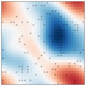
Figure 3: One of the simulated processes at one time instance. Crosses denote the locations that were used to collect the observations. Note that the domain is a torus, that is, a 2-dimensional manifold with periodic boundaries.

Table 1 shows the root-mean-square errors (RMSE) of the mean reconstructions for both the generated gaps and the randomly removed values. The results for each of the five process realizations are shown separately. It appears that using $D=60$ components does not significantly change the performance of the LSSM compared to using $D=30$ components. Also, the LSSM-SD performs practically identically to the LSSM. The LSSM-SD used effectively two or three state dynamics matrices. However, this does not seem to help in modelling the variations in the dynamics and the learned model performs similarly to the LSSM. In contrast to that, the proposed LSSM-TVD has the best performance in each experiment. For the test set of random values, the difference is not large because the reconstruction is mainly based on the correlations between the locations rather than the dynamics. However, in order to accurately reconstruct the gaps, the model needs to learn the changes in the dynamics. The LSSM-TVD reconstructs the gaps more accurately than the other methods, because it finds latent mixing weights $\mathbf{s}_{n}$ which model the changes in the dynamics.

Table 1: Results for five stochastic advection-diffusion experiments. The root-mean-square errors (RMSE) have been multiplied by a factor of 1000 for clarity.

	RMSE for gaps					RMSE for random
Method	1	2	3	4	5	1	2	3	4	5
LSSM $D=30$	104	107	102	94	104	34	38	39	34	34
LSSM $D=60$	105	107	110	98	108	35	39	40	35	35
LSSM-SD $D=30$	106	117	113	94	102	35	37	39	34	34
LSSM-TVD $D=30$	73	81	75	67	82	30	34	35	31	30

Figure 4(a) shows the the posterior distribution of the $K=5$ mixing-weight signals $\mathbf{S}$ in one experiment: the first signal is practically constant corresponding to the average dynamics, the third and the fourth signals correspond to the changes in the two-dimensional velocity field, and the second and the fifth signals have been pruned out as they are not needed. Thus, the method was able to learn the effective dimensionality of the latent mixing-weight process, which suggests that the method is not very sensitive to the choice of $K$ as long as it is large enough. The results look similar in all the experiments with the LSSM-TVD and in every experiment the LSSM-TVD found one constant and two varying components. Thus, the posterior distribution of $\mathbf{S}$ might give insight on some latent processes that affect the dynamics of the observed process.

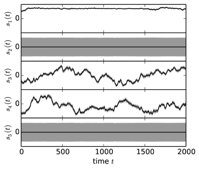
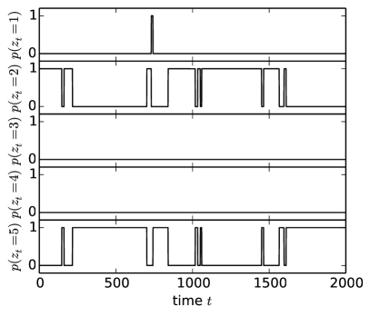
(a) $q(\mathbf{S})$ in LSSM-TVD	(b) $q(\mathbf{Z})$ in LSSM-SD

Figure 4: Results for the advection-diffusion experiments. (a) The posterior mean and two standard deviations of the latent mixing weights by the LSSM-TVD. (b) The posterior probability of each state transition matrix as a function of time in the LSSM-SD.

This experiment showed that the LSSM-SD is not good at modelling linear combinations of the state dynamics matrices. Interestingly, although the VB update formulas average the state dynamics matrices by their probabilities resulting in a convex combination, this mixing is not very prominent in the approximate posterior distribution as seen in Fig. 4(b). Most of the time, only one state dynamics matrix is active with probability one. This happens because the prior penalizes switching between the matrices and one of the matrices is usually much better than the others on average over several time steps.

4.3 Daily Mean Temperature

The third experiment used real-world temperature measurements in Europe. The data were taken from the global surface summary of day product produced by the National Climatic Data Center (NCDC) [18]. We studied daily mean temperature measurements roughly from the European area in 2000–2009. Stations that had more than 20% of the measurements missing were discarded. This resulted in $N=3653$ time instances and $M=1669$ stations for the analysis.

The three models were learned from the data. They used $D=80$ dimensions for the latent states. The LSSM-SD and the LSSM-TVD used $K=6$ state dynamics matrices. We formed two test sets similarly to the previous experiment. First, we generated randomly 300 2-day gaps in the data, which means that measurements from all the stations were removed during those periods of time. Second, 20% of the remaining data was used randomly to form another test set.

Table 2 shows the results for five experiments using different test sets. The methods reconstructed the randomly formed test sets equally well suggesting that learning more complex dynamics did not help and the learned correlations between the stations was sufficient. However, the reconstruction of gaps is more interesting because it measures how well the method learns the dynamical structure. This reconstruction shows consistent performance differences between the methods: The LSSM-SD is slightly worse than the LSSM, and the LSSM-TVD outperforms the other two. Because climate is a chaotic process, the modelling is extremely challenging and predictions tend to be far from perfect. However, these results suggest that the time-varying dynamics might offer a promising improvement to the classical LSSM in statistical modelling of physical processes.

Table 2: GSOD reconstruction errors of the test sets in degrees Celsius for five runs

	RMSE for gaps					RMSE for randomly missing
Method	1	2	3	4	5	1	2	3	4	5
LSSM	1.748	1.753	1.758	1.744	1.751	0.935	0.937	0.935	0.933	0.934
LSSM-SD	1.800	1.801	1.796	1.777	1.788	0.936	0.938	0.936	0.934	0.935
LSSM-TVD	1.661	1.650	1.659	1.653	1.660	0.935	0.937	0.935	0.932	0.934

5 Conclusions

This paper introduced a linear state-space model with time-varying dynamics. It forms the state dynamics matrix as a time-varying linear combination of a set of matrices. It uses another linear state-space model for the mixing weights in the linear combination. This is different from previous time-dependent LSSMs which use switching models to jump between a small set of states defining the model dynamics.

Both the LSSM with switching dynamics and the proposed LSSM are useful but they are suitable for slightly different problems. The switching dynamics is realistic for processes which have a few possible states that can be quite different from each other but each of them has approximately linear dynamics. The proposed model, on the other hand, is realistic when the dynamics vary more freely and continuously. It was largely motivated by physical processes based on stochastic partial differential equations with time-varying parameters.

The experiments showed that the proposed LSSM with time-varying dynamics can capture changes in the underlying dynamics of complex processes and significantly improve over the classical LSSM. If these changes are continuous rather than discrete jumps between a few states, it may achieve better modelling performance than the LSSM with switching dynamics. The experiment on a stochastic advection-diffusion process showed how the proposed model adapts to the current dynamics at each time and finds the current velocity field which defines the dynamics.

The proposed model could be further improved for challenging real-world spatio-temporal modelling problems. First, the spatial structure could be taken into account in the prior of the loading matrix using, for instance, Gaussian processes [19]. Second, outliers and badly corrupted measurements could be modelled by replacing the Gaussian observation noise distribution with a more heavy-tailed distribution, such as the Student-$t$ distribution [20].

The method was implemented in Python as a module for an open-source variational Bayesian package called BayesPy [21]. It is distributed under an open license, thus making it easy for others to apply the method. In addition, the scripts for reproducing all the experimental results are also available.

Acknowledgments.

We would like to thank Harri Valpola, Natalia Korsakova, and Erkki Oja for useful discussions. This work has been supported by the Academy of Finland (project number 134935).

References

- [1] Bar-Shalom, Y., Li, X.R., Kirubarajan, T.: Estimation with Applications to Tracking and Navigation. Wiley-Interscience (2001)
- [2] Shumway, R.H., Stoffer, D.S.: Time Series Analysis and Its Applications. Springer (2000)
- [3] Ghahramani, Z., Roweis, S.T.: Learning nonlinear dynamical systems using an EM algorithm. Advances in neural information processing systems (1999) 431–437
- [4] Valpola, H., Karhunen, J.: An unsupervised ensemble learning method for nonlinear dynamic state-space models. Neural computation 14(11) (2002) 2647–2692
- [5] Ghahramani, Z., Hinton, G.E.: Variational learning for switching state-space models. Neural Computation 12 (1998) 963–996
- [6] Pavlovic, V., Rehg, J.M., MacCormick, J.: Learning switching linear models of human motion. In: Advances in Neural Information Processing Systems 13. MIT Press (2001) 981–987
- [7] Raiko, T., Ilin, A., Korsakova, N., Oja, E., Valpola, H.: Drifting linear dynamics (abstract). In: International Conference on Artificial Intelligence and Statistics (AISTATS 2010). (2010)
- [8] Michalski, V., Memisevic, R., Konda, K.: Modeling sequential data using higher-order relational features and predictive training. arXiv preprint arXiv:1402.2333 (2014)
- [9] Beal, M.J.: Variational algorithms for approximate Bayesian inference. PhD thesis, Gatsby Computational Neuroscience Unit, University College London (2003)
- [10] Luttinen, J.: Fast variational Bayesian linear state-space model. In: Machine Learning and Knowledge Discovery in Databases. Volume 8188 of Lecture Notes in Computer Science. Springer (2013) 305–320
- [11] Bishop, C.M.: Variational principal components. In: Proceedings of the 9th International Conference on Artificial Neural Networks (ICANN’99). (1999) 509–514
- [12] Bishop, C.M.: Pattern Recognition and Machine Learning. 2nd edn. Information Science and Statistics. Springer, New York (2006)
- [13] Beal, M.J., Ghahramani, Z.: The variational Bayesian EM algorithm for incomplete data: with application to scoring graphical model structures. Bayesian Statistics 7 (2003) 453–464
- [14] Barber, D., Chiappa, S.: Unified inference for variational Bayesian linear Gaussian state-space models. In: Advances in Neural Information Processing Systems 19. MIT Press (2007)
- [15] Liu, C., Rubin, D.B., Wu, Y.N.: Parameter expansion to accelerate EM: the PX-EM algorithm. Biometrika 85 (1998) 755–770
- [16] Qi, Y.A., Jaakkola, T.S.: Parameter expanded variational Bayesian methods. In: Advances in Neural Information Processing Systems 19. MIT Press (2007) 1097–1104
- [17] Luttinen, J., Ilin, A.: Transformations in variational Bayesian factor analysis to speed up learning. Neurocomputing 73 (2010) 1093–1102
- [18] NCDC: Global surface summary of day product. http://www.ncdc.noaa.gov/cgi-bin/res40.pl [Online; accessed 16-April-2014].
- [19] Luttinen, J., Ilin, A.: Variational Gaussian-process factor analysis for modeling spatio-temporal data. In: Advances in Neural Information Processing Systems 22. MIT Press (2009)
- [20] Luttinen, J., Ilin, A., Karhunen, J.: Bayesian robust PCA of incomplete data. Neural Processing Letters 36(2) (2012) 189–202
- [21] Luttinen, J.: BayesPy – Bayesian Python. http://www.bayespy.org