1

Two-trace model for spike-timing-dependent
synaptic plasticity

Rodrigo Echeveste¹, Claudius Gros^1
1 Institute for Theoretical Physics, Goethe University Frankfurt, Germany

Abstract

We present an effective model for timing-dependent synaptic plasticity (STDP) in terms of two interacting traces, corresponding to the fraction of activated NMDA receptors and the $Ca^{2+}$ concentration in the dendritic spine of the postsynaptic neuron. This model intends to bridge the worlds of existing simplistic phenomenological rules and highly detailed models, constituting thus a practical tool for the study of the interplay between neural activity and synaptic plasticity in extended spiking neural networks.

For isolated pairs of pre- and postsynaptic spikes the standard pairwise STDP rule is reproduced, with appropriate parameters determining the respective weights and time scales for the causal and the anti-causal contributions. The model contains otherwise only three free parameters which can be adjusted to reproduce triplet nonlinearities in both hippocampal culture and cortical slices. We also investigate the transition from time-dependent to rate-dependent plasticity occurring for both correlated and uncorrelated spike patterns.

Keywords: STDP, spike triplets, frequency dependent plasticity

1 Introduction

The fact that synaptic plasticity can depend on the precise timing of pre- and postsynaptic spikes (Bi et al., 2005; Rubin et al., 2005), indicates that time has to be coded somehow in individual neurons. If the concentration of a certain ion or molecule, which we will refer to as a trace, decays in time after a given event in a regular fashion, then the level of that trace could serve as a time coder, in the same way as the concentration of a radioactive isotope can be used to date a fossil.

A range of models have been proposed in the past that formulate long-term potentiation (LTP) and long-term depression (LTD) in terms of traces in the postsynaptic neurons (Karmarkar et al., 2002; Badoual et al., 2006; Shouval et al., 2002; Rubin et al., 2005; Graupner et al., 2012; Uramoto et al., 2013). Several of these models successfully reproduce a wide range of experimental results; including pairwise STDP, triplet and even quadruplet nonlinearities. Most models, however, require fitting of a large number of parameters individually for each experimental setup and involve heavily non-linear functions of the trace concentrations. While possibly realistic in nature, the study of neural systems modeled under these rules from a dynamical point of view becomes a highly non-trivial task. At the other end, the connection between predictions of simplified models, constructed as phenomenological rules (Badoual et al., 2006; Froemke et al., 2002), and the biological underpinnings is normally hard to establish, as they usually aim to reproduce only the synaptic change and do away with the information stored in the the traces themselves.

In the present work we propose a straightforward model formulating synaptic potentiation and depression in terms of two interacting traces representing the fraction of activated N-methyl-D-aspartate (NMDA) receptors and the concentration of intracellular $Ca^{2+}$ at the postsynaptic spine, with the intention of bridging these two worlds. Having a low number of parameters and being composed of only polynomial differential equations, the model is able nonetheless to reproduce key features of LTP and LTD. Moreover, since the parameters of the model are easily related to the dynamical properties of the system, it permits to make a connection between the observed synaptic weight change and the behavior of the underlying traces.

2 The model

Plasticity in our model will be expressed in terms of two interacting traces on the postsynaptic site, which we denote $x$ and $y$, representing the fraction of open-state NMDA receptors (or NMDARs) and the $Ca^{2+}$ concentration in the dendritic spine of the postsynaptic neuron, respectively. For a clarification we shortly recall the overall mechanism of the synaptic transmission process in a glutamatergic synapse, as illustrated in Fig. 1.

Figure 1: Illustration of a glutamatergic synapse. Primary AMPA receptors (AMPAR) are directly activated by glutamate, voltage gated calcium channels (VGCC) by the backpropagation action potential. NMDA receptors (NMDAR) are also activated by glutamate and allow the influx of calcium if they additionally unblock, which occurs when the backpropagating action potential removes the blocking $Mg^{2+}$ ion.

 

A presynaptic spike results in the release of glutamate molecules across the synaptic cleft, which will activate a series of receptors on the postsynaptic spine, including the already mentioned NMDA receptors, and $\alpha$-amino-3-hydroxy-5-methyl-4-isoxazolepropionic acid (AMPA) receptors (or AMPAR)(Meldrum, 2000). $Na^{+}$ ions will then flow through the AMPAR channels into the dendritic spine of the postsynaptic cell, triggering a cascade of events which may eventually lead to the activation of an axonal spike at the soma of the postsynaptic cell, and of an action potential backpropagating down the dendritic tree. This action potential has two effects captured within our model: the first is the activation of voltage-gated $Ca^{2+}$ channels (VGCC), allowing an influx of $Ca^{2+}$ ions, resulting hence in an increase of the $Ca^{2+}$ concentration $y$; the second is the unblocking of NMDAR channels, as we detail in what follows.

$Ca^{2+}$ ions may flow into the postsynaptic spine also through the NMDAR channels (Meldrum, 2000), but for this to happen two conditions need to be fulfilled. NMDARs are activated when glutamate binds to them, which in turn opens the receptor’s $Ca^{2+}$ permeable channel. The channels are said to be open when the protein’s conformational state permits ions to flow through them, and closed otherwise. At resting membrane potential, however, $Mg^{2+}$ ions are present in the channel’s pore, blocking the channel and preventing $Ca^{2+}$ ions from permeating the neuron (Mayer et al., 1984). This block is temporarily removed by a back-propagating action potential. For $Ca^{2+}$ to flow into the postsynaptic spine two conditions need hence to be fulfilled. The presence of glutamate in the synaptic cleft, triggered by a presynaptic spike, and a back-propagating action potential, signaling a postsynaptic spike. The NMDA receptors are hence the primary agents, within our model, for the interaction of pre- and postsynaptic neural activities in terms of axonal spikes. They are hence also the primary agents for causality within the STDP rule.

2.1 Trace dynamics

We denote with $\{t_{pre}^{\sigma}\}$ and $\{t_{post}^{\sigma}\}$ the trains of pre- and postsynaptic spikes, respectively. The update rules for the fraction $x$ of open but blocked NMDA receptors and the concentration $y$ of postsynaptic $Ca^{2+}$ ions are then given by

$$\left\{\begin{array}[]{lcl}\dot{x}=-\frac{x}{\tau_{x}}+\mathit{E_{x}}(x)\sum_{\sigma}\delta(t-t_{pre}^{\sigma})\\ \dot{y}=-\frac{y}{\tau_{y}}+(x+y_{c})\mathit{E_{y}}(y)\sum_{\sigma}\delta(t-t_{post}^{\sigma})\end{array}\right.$$ (1)

where $\tau_{x}$ and $\tau_{y}$ represent the time constants for the decay of $x$ and $y$ respectively. In absence of presynaptic spikes, glutamate in the synaptic cleft is cleared by passive diffusion and glutamate transporters (Huang et al., 2004). $Ca^{2+}$ concentration in the postsynaptic site will decay, in turn, in absence of postsynaptic spikes (Carafoli, 1987). In our model, each incoming presynaptic spike produces an increase in the number $x$ of open NMDA channels due to glutamate release, and the $Ca^{2+}$ concentration $y$ increases only when a postsynaptic spike is present, viz when a backpropagating action potential reaches the postsynaptic spine. Calcium increase in (1) is composed of two terms; a constant value $y_{c}$, representing the contribution of VGCCs, and a term proportional to the fraction of open NMDA receptors. In this simplified approach, every NMDAR channel still open from the presynaptic spike, is then unblocked by the backpropagating action potential. Therefore the transient calcium current through NMDA receptors is modeled as proportional to $x$.

Figure 2: a) Plot of the limiting factor $\mathit{E}_{x}$, as defined by (2), as a function of the trace concentration, here exemplified by $x$ (the same applies to $y$). b) Plot of the LTP threshold $(y-b)\theta(y-b)$ present in (3).

 

The efficacy factors $\mathit{E_{x}}$ and $\mathit{E_{y}}$ included in (1) are defined as:

$$\mathit{E_{z}}(z)=\theta(z_{b}-z)\,\left(1-\frac{z}{z_{b}}\right),\qquad\theta(z)=\left\{\begin{array}[]{lcl}0\qquad z\leq 0\\ 1\qquad z>0\end{array}\right.$$ (2)

where $z$ is either $x$ or $y$, and determine the efficacy of spikes in increasing trace concentrations. For trace levels above the respective reference values $x_{b}$ and $y_{b}$ no further increase is possible (see Fig. 2 a) and the trace concentration can only decay exponentially. This determines a refractory period, as shown in Fig. 3. The duration of this period is in this case a function of the decay constant of the trace and the magnitude of the overshoot above the reference value. Below this level, $\mathit{E}$ will tend asymptotically to unity as the trace concentration decays. In this way, previous spikes decrease the efficacy of future spikes. Similar mechanisms of reduced spike efficacy have been proposed in the past in models of STDP (Froemke et al., 2002).

Two forces therefore compete to drive nonlinear plasticity in our model: trace accumulation and spike suppression, the latter formulated in the present effective model via a saturation term.

The update rules (1) for the traces are reduced, in the sense that all superfluous constants have been rescaled away, as discussed further in the Appendix.

Figure 3: Illustration of the effect of the limiting factor $\mathit{E}_{x}$ (dashed red line, upper panel), compare Fig. 2 and Eq. (2), on the trace dynamics (solid blue line, lower panel, compare Eq. (1)). Here for the $x$-trace (the behavior is qualitatively the same for $y$). Two spikes $t^{1}_{pre}$ and $t^{2}_{pre}$ are present and indicated as solid green vertical bars, with the height being proportional to $E_{x}$. The system ignores further incoming spike whenever $x>x_{b}$, resulting in respective refractory periods (shaded grey areas). For finite values of $x<x_{b}$ the efficacy of incoming spikes is reduced proportionally to $x_{b}-x$.

 

2.2 Update rules for the synaptic weight

We now formulate the updating rules for the synaptic weight, or synaptic strength, in terms of the trace concentrations. To this end we consider the contribution of two pathways mediated by distinct enzymes (Colbran, 2004); which, for simplicity we will denote as LTP and LTD pathways. Calcium is involved in both the LTP and the LTD pathways (Cormier et al., 2001; Neveu et al., 1996; Yang et al., 1999), with high levels of calcium resulting in LTP and moderate and low levels resulting in LTD. We propose the following rule for the plasticity of the synaptic weight $w$,

$$\dot{w}=\alpha x(y-b)\theta(y-b)\sum_{\sigma}\delta(t-t_{post}^{\sigma})-\beta xy\sum_{\sigma}\delta(t-t_{pre}^{\sigma}),$$ (3)

with $\theta$ being the same previously defined step function which, in this case, serves as a lower bound. The first term in (3) leads to an increase of the synaptic weight; it is triggered in the presence of a postsynaptic spike and by the calcium concentration $y$, but only if $y$ is larger than a given threshold $b$, see Fig. 2 b). A threshold in the calcium concentration $Ca^{2+}$ for LTP has been experimentally observed (Cormier et al., 2001) and its dependence with the previous synaptic activity has been studied (Huang et al., 1992). In the present work we will consider a constant $b=y_{c}$, and we will show in the next section that the standard STDP curve is obtained with this choice.

The second term in (3), in turn, leads to decrease of the synaptic weight and needs a finite level for both the calcium concentration $y$ and for the fraction of open NMDA receptors $x$ (which can be taken as a measure of the glutamate concentration in the synaptic cleft), in addition to the presence of a presynaptic spike, which acts as a second coincidence detector as proposed by Karmarkar et al. (2002). The parameters $\alpha>0$ and $\beta>0$ represent the relative strengths of these two contributions.

The pre- and postsynaptic spikes $t_{pre/post}^{\sigma}$ mark the timing of the synaptic update in our model (3) for the synaptic plasticity. Here we considered $\delta$-like spikes and one needs, for numerical simulations using small but finite time steps, to update the traces via (1) before updating the weights via (3).

2.3 The pairwise STDP rule

In the limit of low frequencies, the traces decay to zero in between the occurrence of two pairs of spikes, which may hence be considered as isolated.

We denote with $\Delta t$ the time between the pre- and the postsynaptic spike, with a positive value corresponding to a causal pre-post order and a negative $\Delta t$ to an anti-causal post-pre ordering. For an isolated pair of spikes one can easily integrate (1) and (3), obtaining:

$$\Delta w=\left\{\begin{array}[]{lrcl}\alpha\mathrm{e}^{-|\Delta t|/\tau_{x}}\left(\mathrm{e}^{-|\Delta t|/\tau_{x}}+y_{c}-b\right)&\Delta t&>&0\\ -\beta y_{c}\mathrm{e}^{-|\Delta t|/\tau_{y}}&\Delta t&<&0\end{array}\right.$$ (4)

The synaptic weight is always depressed for an anti-causal time ordering of the spikes with $\Delta t<0$, and potentiated for $y_{c}\geq b$ and a causal time ordering corresponding to $\Delta t>0$. The LTP term becomes a simple exponential decay for $b=y_{c}$. We have chosen in our model a fully decoupled formulation for LTP and LTD. While the LTD term is always negative, the restriction on the LTP term to be always positive could be relaxed by removing the step function in equation (3). Then, with the choice $b>y_{c}$, a depression window would arise after the peak of potentiation. This window has indeed been observed in the past in CA1 cells from rat hippocampal slices (Nishiyama et al., 2000). By setting $b<y_{c}$, on the other hand, the decay would be composed of two exponentials. In the LTD term we have not included a threshold. Alternatively, one could replace the calcium level $y$ by an expression $(y-b_{LTD})\theta(y-b_{LTD})$, analogous to the LTP term, which is identical to the case we present for $b_{LTD}=0$ since $y$ is always positive. It is however worth discussing the cases where $b_{LTD}\neq 0$. Apart from the step function $\theta$, the LTD threshold represents only a vertical shift of the negative portion of the STDP window by a factor $\beta b_{LTD}$. If $b_{LTD}<0$ the plot is shifted downwards, which means depression occurs even for isolated presynaptic spikes ($\Delta t\rightarrow-\infty$). This is usually not the case, as seen in Bi et al. (1998) and Froemke et al. (2002). If $b_{LTD}<0$, on the other hand, the plot is shifted upwards but, because of the step function, the $LTD$ term is always negative and then the tail of the exponential would be cut-off. By looking at the experimental results in Figs. 4 and 6, one observes that the data seems in fact quite noisy to determine the exact shape of the decay functions. In absence of further detail, we have chosen in the present work to keep $b=y_{c}$ and no threshold (or a threshold at $0$) for LTD, therefore respecting the exponential fits proposed in the original papers (Bi, 2002; Froemke et al., 2002).

Rewriting the constants $\alpha$, $\beta$, $\tau_{x}$, and $\tau_{y}$ as $\alpha=A^{+}$, $\beta=A^{-}/y_{c}$, $\tau_{x}=2\tau_{+}$, and $\tau_{y}=\tau_{-}$ where $A^{+}$, $A^{-}$, $\tau_{+}$ and $\tau_{-}$ represent the maximal intensities and timescales of LTP and LTD for isolated spike pairs, we obtain with

$$\Delta w=\left\{\begin{array}[]{lrcl}+A^{+}\mathrm{e}^{-|\Delta t|/\tau_{+}}&\Delta t&>&0\\ -A^{-}\mathrm{e}^{-|\Delta t|/\tau_{-}}&\Delta t&<&0\end{array}\right.$$ (5)

the classical fit for pairwise STDP proposed both in hippocampal and cortical neurons (Bi, 2002; Froemke et al., 2002). This result is independent of $y_{c}$, $x_{b}$, and $y_{b}$ and these three parameters can be hence be used to reproduce additional experimental observations. In what follows we will use the amplitudes $A^{\pm}$ as primary parameters, instead of $\alpha$ and $\beta$ and rewrite the plasticity rule (3) as

$$\dot{w}=A^{+}x(y-y_{c})\theta(y-y_{c})\sum_{\sigma}\delta(t-t_{post}^{\sigma})-\frac{A^{-}}{y_{c}}xy\sum_{\sigma}\delta(t-t_{pre}^{\sigma}).$$ (6)

This is the final shape of the equation for the evolution of the synaptic strength that we will use throughout this work, it allows to interpret the results for a variety of spike pattern situations in terms of the known spike-pair STDP parameters. The representations (6) and (3) are, in any case, equivalent.

2.4 Spike triplets

The effect of a pair of pre- and postsynaptic spikes has been experimentally shown to depend, in a non-linear fashion, not only on its inter-spike interval but also on the presence of additional spikes temporally proximal to the pair. The contribution of spike triplets, the simplest case of spike-pair interactions, cannot be described as a linear sum of two individual contributions of spike-pairs (Froemke et al., 2002; Wang et al., 2005).

In the following sections, we will study the model’s results for either two pre- and one postsynaptic spikes in a pre-post-pre order, or one pre- and two postsynaptic spikes in a post-pre-post ordering. For example, with 15Post5 we denote a pre-post-pre ordering,

$$15\mathrm{Post}5,\qquad\quad\left\{t_{pre}^{\sigma}\right\}=\{-15,5\},\qquad\quad\left\{t_{post}^{\sigma}\right\}=\{0\}$$ (7)

and with 10Pre20 a post-pre-post ordering,

$$10\mathrm{Pre}20,\qquad\quad\left\{t_{pre}^{\sigma}\right\}=\{0\},\qquad\quad\left\{t_{post}^{\sigma}\right\}=\{-10,20\}~{},$$ (8)

where the times $t_{pre/post}^{\sigma}$ of the spikes are given in milliseconds.

As for spike pairs, the weight-change induced by low-frequency triplets can be computed analytically, obtaining

$$\begin{array}[]{rcl}\Delta w=&+&A^{+}exp\left(-\frac{\rvert\Delta t_{1}\rvert}{\tau_{+}}\right)\\ &-&A^{-}exp\left(-\frac{\rvert\Delta t_{2}\rvert}{\tau_{-}}\right)\left[1+\frac{exp\left(-\frac{\rvert\Delta t_{1}\rvert}{\tau_{x}}\right)}{y_{c}}\right]\left[1+exp\left(-\frac{\rvert\Delta t_{1}\rvert+\rvert\Delta t_{2}\rvert}{\tau_{x}}\right)\left(1-\frac{1}{x_{b}}\right)\right]\end{array}$$ (9)

for pre-post-pre triplets, and

$$\begin{array}[]{rcl}\Delta w=&-&A^{-}exp\left(-\frac{\rvert\Delta t_{1}\rvert}{\tau_{-}}\right)\\ &+&A^{+}exp\left(-\frac{\rvert\Delta t_{2}\rvert}{\tau_{+}}\right)\left[1+y_{c}exp\left(-\frac{\rvert\Delta t_{1}\rvert+\rvert\Delta t_{2}\rvert}{\tau_{y}}+\frac{\rvert\Delta t_{2}\rvert}{\tau_{x}}\right)\left(1-\frac{exp\left(-\rvert\Delta t_{2}\rvert/\tau_{x}\right)+y_{c}}{y_{b}}\right)\right]\end{array}$$ (10)

for post-pre-post triplets, where we have assumed that the traces are below their respective reference levels, $x_{b}$ and $y_{b}$ respetively, by the time a second spike arrives (the case of the second spike arriving while the trace is above the reference level is discussed later in this section). The saturation effect can reduce the effect of a new spike to zero but not reverse the sign, as seen in expression (2).

We see that the first term in Eqs. (9) and (10), corresponding to the first pair, remains in both cases unchanged, by construction, with non-linearities appearing in the second contribution. In the second term of Eq. (9), we find a first factor (the first parenthesis) corresponding to a correction produced by the interaction between the two traces (the calcium inflow through NMDAR channels), and a second factor corresponding to the balance between trace accumulation and spike suppression. In Eq. (10) we also find a term balancing trace accumulation and spike suppression. The multiplicative factor $exp(\rvert\Delta t_{2}\rvert/\tau_{x})$ inside the brackets comes from the way we have decided to factorize the equation, since $\tau_{x}=2\tau_{+}$.

If the third spike would instead come within the respective refractory period (see Fig. 3), the expressions (9) and (10) would reduce to

$$\begin{array}[]{rcl}\Delta w=&+&A^{+}exp\left(-\frac{\rvert\Delta t_{1}\rvert}{\tau_{+}}\right)\\ &-&A^{-}exp\left(-\frac{\rvert\Delta t_{2}\rvert}{\tau_{-}}\right)\left(1+\frac{exp\left(-\frac{\rvert\Delta t_{1}\rvert}{\tau_{x}}\right)}{y_{c}}\right)exp\left(-\frac{\rvert\Delta t_{1}\rvert+\rvert\Delta t_{2}\rvert}{\tau_{x}}\right)\end{array}$$ (11)

for pre-post-pre triplets, and:

$$\Delta w=-A^{-}exp\left(-\frac{\rvert\Delta t_{1}\rvert}{\tau_{-}}\right)$$ (12)

for post-pre-post triplets, where in Eq. (12) the second pair is directly inhibited by the LTP threshold. While this last situation is not encountered for the low frequency triplet configurations presented in this work, it becomes relevant in high frequency scenarios. This condition could be relaxed by replacing the strict threshold by a smooth sigmoidal.

2.5 Interpretation of the variables and parameters in the model

The here proposed model contains a relative small number of variables and parameters and can be considered an effective approach with the biological underpinnings of STDP being governed by a substantially larger number of variables and parameters whose functional interdependences are naturally far more complex than the polynomial descriptions here proposed. Any effective model will however pool together within each effective variable or parameter several effects which might depend on a variety of different factors in the biological neuron.

In section 2.1, we defined $x$ as the fraction of open but unblocked NMDAR channels. When paired with a postsynaptic spike, and under the simplifications assumed in the model, the value of $x$ can be then associated with a transient calcium current and a comparison with experimental results of the parameters related to $x$ would reflect this role. The time window for LTP, for instance, results in our model from the value of $\tau_{x}=2\tau_{+}$ (as we showed in section 2.3). $\tau_{x}$ can then be interpreted in this context as the decay time of the transient calcium current. It has been argued by Hao et al. (2012) that the narrow window for LTP results from AMPA-EPSP in the postsynaptic spine. In fact, as reviewed in the same article, the whole spine seems to work as an electrical amplifier, locally prolonging the depolarization time at the spine. It is therefore not surprising to find different values of the time constants in different neurons or even within different synapses within the same neuron. In our model we do not compute AMPA currents directly and reduce the overall effect of the spine to the effective value of $\tau_{x}$. Similarly, $\tau_{y}$ represents the timescale for decay of the effective calcium concentration at the spine.

We have included in this work saturation terms for both variables $x$ and $y$. As it has been proposed in the past (Froemke et al., 2002), triplet nonlinearities in visual cortical neurons indicate strong suppression effects on future spikes by previous spikes of the train. The saturation terms included in the model provide one possible effective way of dealing with spike suppression, reducing a biological complex phenomena further down the cascade of processes, leading eventually to LTP and to LTD respectively.

3 Results for the Hippocampus

Our model, as defined by (1) and (6) contains overall seven adjustable parameters. Four of these parameters, namely $A^{+}=\alpha$, $A^{-}=\beta/y_{c}$, $\tau_{+}$, and $\tau_{-}$, enter explicitly the isolated spike-pair STDP rule (5) and are determined directly by experiment. For cultured rat hippocampal neurons

$$A^{+}=0.86/60,\qquad A^{-}=0.25/60,\qquad\tau_{+}=19\,\mathrm{ms},\qquad\tau_{-}=34\mathrm{\,}{ms}$$ (13)

have been measured (Bi, 2002) and we will use these experimental values throughout the hippocampus part of this study. In Fig. 4 we present, as an illustration, both the experimental and the theory results, with the latter reproducing, by construction, the experimental fit. For the model simulation, the experimental protocol of 60 repetitions spaced by one second has been used. However, the $1\mathrm{Hz}$ frequency of spike pairs is so low that (5) could be directly used without any discernible difference.

Figure 4: Weight change after a train of 60 pairs at a constant frequency of $1\,\mathrm{Hz}$ as a function of the time delay $\Delta t$ between pre- and postsynaptic spikes. The red open circles are the experimental data for hippocampal neurons (Bi et al., 1998). The continuous blue line represents the model’s results when the parameters are set to $A^{+}=0.86/60$, $A^{-}=0.25/60$, $\tau_{+}=19\mathrm{ms}$, $\tau_{-}=34\mathrm{ms}$, which correspond to a fit of the experimental data, as presented in Bi (2002).

 

Three parameters entering (1) and (6), namely $y_{c}$, $x_{b}$, and $y_{b}$ are to be selected. In a continuous time evolution scenario, $x_{b}$ and $y_{b}$ determine strict maximal concentrations for the traces. In the discrete time scenario, overshoots are however possible, due to the finite increase in the traces after every spike. In this context, and in a low frequency situation, the first spike in the stimulation pattern is unaffected by the limiting factor, and only the efficacy of the following spike is reduced. Since $x_{b}$ and $y_{b}$ then do not affect pairwise STDP, they need to be selected from higher order contributions to the weight-change. In this case, we selected the values of $y_{c}$, $x_{b}$, and $y_{b}$ from triplet results, as presented in what follows.

In Fig. 5 we now compare our results for triplets, as described in section 2.4, with experiments for cultured rat hippocampal neurons (Wang et al., 2005). The triplet stimulation experimental protocol consists of a regular train of 60 triplets with a repetition frequency of $1\,\mathrm{Hz}$ and we use the identical protocol for the theory simulations. We also keep the pairwise STDP parameters (13) valid for cultured rat hippocampal neurons and adjust the remaining three free parameters $y_{c}$, $x_{b}$, and $y_{b}$ by minimizing the standard deviation (SD) between the numerical and the experimental results, obtaining $y_{c}=0.28$, $y_{b}=0.66$, and $x_{b}=0.62$ (with an SD of $6.76$).

Figure 5: Synaptic strength change in hippocampal neurons induced by triplets composed of either two pre- and one postsynaptic spike, left side of the diagram, compare (7), or one pre- and two postsynaptic spikes, right side of the diagram, see (8). A total of 60 triplets are presented, with a repetition frequency of $1\,\mathrm{Hz}$. Full blue boxes correspond to the model’s results, empty red bars to experimental data (Wang et al., 2005), and the green lines represent the linear addition of the PostPre and PrePost pairs each triplet contains via (6). Simulation parameters: $A^{+}=0.86/60$, $A^{-}=0.25/60$, $\tau_{+}=19\mathrm{ms}$, $\tau_{-}=34\mathrm{ms}$, $y_{c}=0.28$, $x_{b}=0.62$, and $y_{b}=0.66$.

 

We found that the SD varies smoothly, and relatively weakly, with the exact choice of the three free parameters, as can be expected from the analytical expressions, and that this freedom can be used to obtain a range of functional dependencies of the synaptic plasticity upon spiking frequencies, as discussed in Sect. 5.

We have also included in Fig. 5 the expected synaptic weight changes for the case of a linear superposition of the two respective interspike contributions via (6). One observes that the discrepancy between the non-linear and the linear interactions is much stronger for pre-post-pre than for post-pre-post triplets. With the former leading to an overall reduced synaptic weight change and the later configuration to a substantial potentiation. It is interesting to observe here that spike suppression, as proposed in Froemke et al. (2002) from cortical neurons cannot explain nonlinearities in hippocampus. Suppression of the second presynaptic spike in the triplet would reduce depression and the overall result would be supralinear potentiation, contrary to the experimental observation. Trace accumulation is the dominant effect driving nonlinearities in hippocampal neurons.

4 Results for the Cortex

We repeat now the procedure presented previously for the hippocampus, comparing the results of the proposed plasticity rule to experimental data obtained from slices of the visual cortex. As in the previous section, the values of $A^{+}=\alpha$, $A^{-}=\beta/y_{c}$, $\tau_{+}$, and $\tau_{-}$ are determined directly by experiment. We use

$$A^{+}=1.03/60,\qquad A^{-}=0.51/60,\qquad\tau_{+}=13.3\,\mathrm{ms},\qquad\tau_{-}=34.5\mathrm{\,}{ms}$$ (14)

as obtained by Froemke et al. (2002) for pyramidal neurons in layer 2/3 (L2/3) of rat visual cortical slices. Both experiment and the STDP curve are shown in Fig. 6, where we have reproduced, for the simulation, the experimental protocol, using 60 repetitions at $0.2\,\mathrm{Hz}$. Once again, the frequency of spike pairs is so low that (5) could be directly used without any discernible difference.

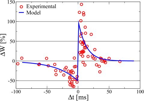
Figure 6: As in Fig. 4, now for visual cortical neurons. The stimulation frequency is now $0.2\,\mathrm{Hz}$, as in the experiment (Froemke et al., 2002). The red open circles are the experimental data (courtesy of Robert C. Froemke and Yang Dan) and the continuous blue line represents the model’s results when the parameters are set to $A^{+}=1.03/60$, $A^{-}=0.51/60$, $\tau_{+}=13.3\,\mathrm{ms}$, $\tau_{-}=34.5\mathrm{\,}{ms}$, corresponding to the fit of the experimental data presented in Froemke et al. (2002).

 

To select $y_{c}$, $x_{b}$, and $y_{b}$ we once again resort to triplet results. In Froemke et al. (2002), the change produced by triplets of either two pre- and one postsynaptic spikes or one pre- and two postsynaptic spikes was also measured. The data consist in this case however of a large set of specific triplet timing configurations, with every individual triplet configuration measured once. We decided to treat all measurements on an equal footing, fitting the complete set by minimizing the mean square error without introducing any further bias.

Figure 7: As in Fig. 5, now for visual cortical neurons. The stimulation frequency is now $0.2\,\mathrm{Hz}$ as in the experiment (Froemke et al., 2002). Full blue boxes correspond to the model’s results for the best fit of the parameters, empty red bars to experimental data, and the green lines represent the linear addition of the two PostPre and PrePost pairs each triplet contains. With diamonds, the model’s results for an alternative set of parameters is presented. While the quantitative differences are larger with this parameter choice, the model still qualitatively reproduces cortical triplet nonlinearities. Simulation parameters: $A^{+}=1.03/60$, $A^{-}=0.51/60$, $\tau_{+}=13.3\,\mathrm{ms}$, $\tau_{-}=34.5\mathrm{\,}{ms}$, Best fit: $y_{c}=11.6$, $y_{b}=10.9$, and $x_{b}=0.5$. Diamond points: $y_{c}=1.0$, $y_{b}=0.9$, and $x_{b}=0.4$.Experimental data courtesy of Robert C. Froemke and Yang Dan.

 

We obtain in this case $y_{c}=11.6$, $y_{b}=10.9$, and $x_{b}=0.5$. The obtained SD of $37.4$ is, in this case, much larger than the one found for hippocampus, though that is partly due to the variance in the experimental data themselves, corresponding to individual data points and not to averaged results. Another consequence of the large variance in the data is that the minimum in the SD is relatively broad. We will discuss these points in detail in what follows.

In order to compare the results for cortical neurons with the previous section on hippocampal neurons, as presented in In Fig. 5, we have performed a smooth interpolation of the set of individual experimental results for cortical triplets by means of gaussian filters. In Fig. 7 we compare the theory results with the interpolated experimental data.

Contrary to hippocampal triplet results presented in Fig. 5, experiments in cortical slices show that post-pre-post triplets lead to strong depression and pre-post-pre triplets to potentiation. Post-pre-post triplets deviate, in addition, somewhat more from a linear superposition of the contribution of the two inherent spike pairs than the pre-post-pre configuration. While the predictions of the model presented in Fig. 7) are clearly not as good as the ones obtained for hippocampal culture, they are still qualiatively in agreement with the experimental results, successfully capturing the asymmetry between post-pre-post and pre-post-pre triplets. While, there is still room for improvement in this regard, we believe it is important that the model can switch from the hippocampal to the cortical regime in terms of triplet nonlinearities.

As we previously mentioned, the data itself has a much larger variance in this case. To have an idea of of the variability of the data, we computed the standard deviation of the data to the smooth gaussian interpolation of width 5ms that we used for the visual comparison of Fig. 7, which yields an SD of $32.5$ (as compared to the SD of $37.4$ between model and experiment). For this reason, we believe that a reasonable goal in this case is to reproduce the distinct qualitative feature of the triplet nonlinearities, more than an accurate quantitative approximation.

The optimal value of $y_{c}=11.6$ obtained when fitting the experimental triplet results, see Fig. 7, seems to be too large, in particular when compared to the one obtained for hippocampal neurons. This result can be traced back to the occurrence of a broad minimum for the least-square fit together with a relative high variability of the experimental data. We have hence also examined parameter configurations with lower values for $y_{c}$. Also included in Fig. 7 is an example with $y_{c}=1.0$, also representing the observed experimental features qualitatively. We find that the particular cortical structure of triplets arises from strong saturation, being a consequence of $y_{b}<y_{c}$.

5 Frequency dependence

So far, we have considered only pairs or triplets of pre- and postsynaptic spikes coming at low frequencies and with very precise timings. This will not necessarily be the case in a natural train of spikes. It is therefore interesting to examine the model’s prediction for spike trains with different degrees of correlation between pre- and postsynaptic spikes. A neuron usually receives input from about ten thousand other neurons. While the correlation of the postsynaptic neuron will be higher for a strong synapse driving the neuron, the postsynaptic neuron will in general not be correlated with all of its inputs. We therefore study both types of connections.

We begin in section 5.1 by studying the case of uncorrelated trains of pre- and postsynaptic spikes and then analyze in section 5.2 the case of a driving synapse with different degrees of correlation. In these sections we numerically evaluate the synaptic strength change as a function of the pre- and postsynaptic neuronal firing rates.

5.1 Plasticity induced by uncorrelated spikes

We begin by evaluating the synaptic change produced by uncorrelated trains of Poisson pre- and postsynaptic spikes. In these simulations we use the same parameters as fitted from pairwise and triplet experiments in Hippocampus and Cortex, refering to hippocampal and cortical neurons respectively.

The results of the simulations for hippocampal neurons are presented in Fig. 8. We present two kinds of plots in the diagram: a plot where the pre- and postsynaptic firing rates are equal, and plots of constant presynaptic frequency for varying postsynaptic firing rate. We observe in this last type, that the sign of the weight changes, as a function of the postsynaptic activity for a constant presynaptic frequency, generically switching from negative to positive at a certain threshold $\theta_{H}$. This threshold increases with rising presynaptic frequency, resulting in a sliding threshold. In other rate-based learning rules like BCM (Bienenstock et al., 1982), similar thresholds for potentiation are determined by appropriate long term averages of the postsynaptic activity. In our model, $\theta_{H}$ is set by the level of the presynaptic activity, as measured on timescales of the respective traces. This feature would allow the neuron to adjust the threshold of each synapse independently, setting in each case the level of what constitutes a significant activity.

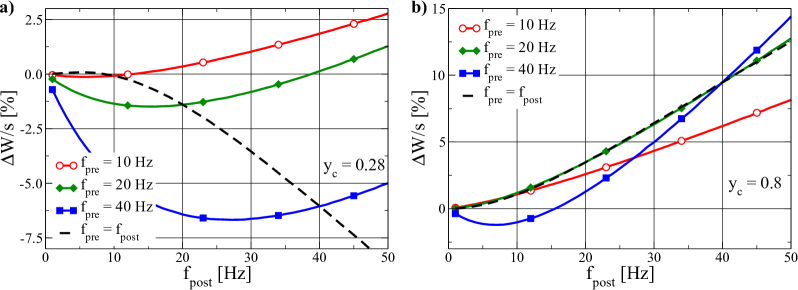
Figure 8: Average weight change, for hippocampal neurons, produced by one-second trains of uncorrelated Poisson-distributed pre- and postsynaptic spikes, as a function of the postsynaptic firing frequency $f_{post}$ and for various constant presynaptic firing rates $f_{pre}$ (full lines). Also included is the case for identical pre- and postsynaptic firing rates (dashed line). The pair-STDP values (13) have been used and two sets of values for the remaining three free parameters, yielding both otherwise very similar results for the spike triplets. a) $y_{c}=0.28$, $y_{b}=0.66$, and $x_{b}=0.62$. b) $y_{c}=0.8$, $y_{b}=1.34$, and $x_{b}=1.82$.

 

The overall synaptic change becomes Hebbian for large pre- and post- firing rates $f_{pre}$ and $f_{post}$, in the sense that it is then proportional to the product $f_{pre}\cdot(f_{post}-\theta_{H})$. This weight change is influenced in a substantial way by the value of $y_{c}$ and we have presented in Fig. 8 two sets of parameters, one with $y_{c}=0.28$ (left panel) and one with $y_{c}=0.8$ (right panel), yielding otherwise similar SDs when fitting the experimental triplet data ($6.76$ and $7.37$ respectively).

Potentiation dominates for larger values of $y_{c}$, as seen in Fig. 8 b). These results seem, at first sight, counterintuitive given the role of $y_{c}$ as a threshold for LTP. Note however, that $y_{c}$ contributes to the increase in $y$ through (1) and both LTP and LTD are dependent on $y$ in the plasticity rule (6), with the LTD contribution being proportional to $1/y_{c}$.

Comparing Figs. 8 a) and b) we observe that $y_{c}$ can be used to regulate the threshold for potentiation in the rate-encoding limit, without changing the behavior of isolated spike triplets substantially. $y_{c}$ is hence a vehicle for also adapting the overall postsynaptic activity level and it would be interesting, for future research, to study how this regulative mechanism would interact with other known ways to regulate the overall level of the postsynaptic neural activity, such as intrinsic plasticity rules (Triesch, 2007; Marković et al., 2012; Linkerhand et al., 2013).

Figure 9: As in Fig. 8, now for visual cortical neurons. Full lines show the weight change for specific constant presynaptic frequencies $f_{pre}$, as a function of the postsynaptic rate $f_{post}$. For the dashed line, pre- and postsynaptic firing rates are equal. The pair-STDP values (14) have been used and two sets of values for the remaining three free parameters, yielding both otherwise similar results for the spike triplets. a) $y_{c}=11.6$, $y_{b}=10.9$, and $x_{b}=0.5$. b) $y_{c}=1.0$, $y_{b}=0.9$, and $x_{b}=0.4$.

 

It has to be remarked that the full lines in Fig. 8, representing weight changes as a function of the postsynaptic frequency for a constant presynaptic firing rate, while of theoretical interest to understand the behaviour of $\theta_{H}$, will not correspond to a usual physiological functional relationship between the rates, at least for a driving synapse. If the presynaptic synapse drives the postsynaptic neuron, the postsynaptic activity will in general be an increasing function of the presynaptic rate. Here we have chosen $f_{pre}=f_{post}$ (the dashed lines in Fig. 8 and 9) as an illustration, but a more detailed transfer function should be selected for accurate and quantitative comparisons with experimental results. In this sense, the parameter configuration of Fig. 8 b) shows a better agreement with experimental procedures, such as that of Sjöström et al. (2001), where potentiation is shown to become stronger with higher frequencies.

No complete set of experimental results has hitherto been published, unfortunately, where all pairwise, triplet, and frequency dependent plasticity have been measured for the same type of synapse and with the same experimental stimulation procedure. A full consistency check between model and experiment is hence not possible to date.

In Fig. 9 the results of numerical simulations for L2/3 cortical neurons for the same protocol of Fig. 8 are presented. In this case, depression is found for all combinations of pre- and postsynaptic frequencies, a robust prediction of the model. Different values of $y_{c}$ were selected to test this behavior, and in each case the rest of the parameters were fitted to the triplet results. In each case, the value of $y_{b}$ obtained by this fitting turned out to be lower than $y_{c}$. The $y$-trace has hence a hard time to overcome the threshold $y_{c}$ for LTP, as calcium increase by further spikes is prevented. As a test, if $y_{b}$ was artificially set to values larger than $y_{c}$, potentiation for larger frequencies was recovered but the fit of the experimental triplet data deteriorated substantially, obtaining potentiation for PostPrePost triplets, contrary to the experimental results. This indicates that triplet nonlinearities found in L2/3 cortical neurons result from spike suppression, contrary to the predominant trace accumulation effect present in hippocampal neurons.

These results, predicted for L2/3 neurons as fitted from Froemke et al. (2002), would then be in stark contrast to those of Sjöström et al. (2001) for L5 neurons in visual cortex where LTP dominates for large frequencies. It should be pointed out, however, that the pairwise STDP plot presented in Sjöström et al. (2001) is already different from that of L2/3 neurons, raising the question of to what extent results coming from different neurons, or obtained via different stimulation procedures, should be alike.

On the other hand, the prediction of overall depression dominating for uncorrelated spike trains in certain cortical neurons seems to be in line with, or at least does not contradict, experimental findings for deprivation experiments. In cortical areas, where topological maps are usually found, deprivation of sensory input has been shown to result in depression of the respective synaptic connections (Trachtenberg et al., 2000; Feldman, 2000). At the same time, correlation has been found to substantially decrease after these procedures, in areas projecting to cortex (Linden et al., 2009), suggesting that decorrelation of spike trains could be responsible for the observed depression in cortical neurons.

A possible reason behind the observed differences in these studies might be the stimulation protocol employed. While in Bi et al. (1998) and Wang et al. (2005), plasticity is triggered by eliciting the firing of the pre- and postsynaptic neurons by dual whole-cell clamp, in the cortical results from Froemke et al. (2002), extracellular presynaptic stimulation is performed, clamping only the postsynaptic neurons. This creates an asymmetry between Pre-Post-Pre and Post-Pre-Post triplets. Moreover, in the case of extracellular stimulation, the question remains to what extent other synapses are being affected, potentially triggering, in turn, other forms of plasticity such as local synaptic scaling.

It is important to stress that the robust depression found here for higher frequencies is a direct consequence of the triplet results, and indeed vanishes if one uses hippocampal-like triplet results. The same suppression effect present for triplets also affects higher frequency trains, resulting in depression.

For lower frequencies, the pairwise contribution dominates when determining the balance between potentiation and depression. In Izhikevich et al. (2003), the authors show how a straightforward application of the pairwise rule to Poisson uncorrelated spike trains (as in our simulation), adding up linearly the effect of every pair in the train according to the pairwise STDP rule with cortical parameters, always leads to depression, since the pairs simply sample the STDP curve which has an overall negative area (the opposite is true in hippocampal neurons, as we show below). Our model is by construction, equivalent in the low frequency limit to the linear pairwise model since isolated spikes produce no synaptic change in our model and triplets and higher order configurations become very infrequent if the frequency is low. For low pre- and postsynaptic frequencies the trains of Poisson spikes can be considered as pairs of random duration that sample the pairwise STDP curve.

As previously mentioned, the overall integrated area of the pairwise STDP curve for L2/3 cortical neurons is negative while it is positive for hippocampal neurons. One can easily integrate the exponentials and one obtains a relation $A$ for the areas:

$$A=\frac{A^{+}\tau_{+}}{A^{-}\tau_{-}}.$$ (15)

While for hippocampal neurons $A=1.92$, we find in cortex $A=0.77$. This means that, in absence of higher order contributions (which is true if both the pre- and the postsynaptic frequencies are low), uncorrelated spikes will on average lead to depression in cortical neurons and to potentiation in hippocampal neurons. If the frequencies tend to zero, the average interspike interval will be long compared to the STDP window duration and the net amount of synaptic change, whether positive or negative, will be low. In the following section this fact will become clear when the synaptic change of correlated and uncorrelated spikes are compared.

As the frequencies of pre- and postsynaptic spikes increase, the interspike period decreases and when this becomes comparable to the timescale of the STDP window (which is related to the trace timescale), the pairwise approximation will break down since interactions can no longer be neglected. When both the pre- and postsynaptic frequencies are on the order of $10\mathrm{Hz}$ the average time between a pre- and a postsynaptic spike is on the order of $50\mathrm{ms}$ and interactions are to be expected. This is where the particular models for the underlying dynamics will differ. Also in the work by Izhikevich et al. (2003), the authors show with their Nearest-neighbor Implementation that synaptic change goes from general depression (in the all-to-all implementation) to BCM-like, when they consider only the closest previous and posterior postsynaptic spike to each presynaptic spike to compute the linear sum of pairs.

This choice, which at first glance would seem an approximation independent of any underlying dynamics, actually has strong implications for the biological underpinnings that could actually implement this algorithm. A first neighbor approximation requires to hard reset any traces possibly present, forgetting completely anything that happened outside that window. The nearest-neighor implementation has, in addition not the aim to explain triplet non-linearities as the PrePostPre triplet protocol.

The interspike interaction is in our model driven by the undelying traces. We have chosen in our simulation to use for the frequency-dependence protocol the same parameters obtained from pairwise and triplet fits. As observed in cortical PostPrePost triplets, strong suppression severely limits potentiation of further spikes (compare PostPrePost to linear superposition results). At high frequencies triplet interactions become relevant and the same suppression should then be evidenced for frequency dependent plasticity. We believe then, that any model aiming to reproduce time-dependent plasticity up to triplet order as measured by Froemke et al. (2002), should show depression also for high frequencies in cortical neurons.

5.2 Plasticity induced by correlated spikes

So far we have analyzed the effect of uncorrelated spikes on the synaptic weight change both in hippocampal and in cortical neurons (Figs. 8 and 9). It is however interesting to see the predictions of the model for a strong synapse driving the postsynaptic neuron. In this case pre- and postsynaptic spikes should be correlated, at least partially, together with a certain positive delay.

To reproduce this effect with our model, we simulated trains of correlated spikes where, with each presynaptic spike, a postsynaptic spike can occur with probability $p$, after a certain delay $d$. As an example, if every presynaptic spike triggers a postsynaptic spike then $p=1$. This would mean, however that the postsynaptic frequency $f_{post}$ changes with $p$ ($f_{post}=p$ $f_{pre}$). In order to compare our results for different values of $p$ and keep $f_{post}$ independent of $p$, we complete the train of postsynaptic spikes with Poisson spikes of frequency $(1-p)f_{pre}$. In this way, $f_{post}$ is independent of $p$, which now regulates the degree of correlation between pre- and postsynaptic spikes: $p=0$ represents the fully decorrelated case, since all the postsynaptic spikes are drawn from the poisson distribution, and $p=1$ represents the fully correlated case already mentioned.

In Fig. 10 we present the synaptic changes produced by trains spikes for different values of $p$. In this case, results for a delay of $5\mathrm{ms}$ are presented. The same tests were performed with delays from $2\mathrm{ms}$ to $10\mathrm{ms}$ with only quantitative but not qualitative differences.

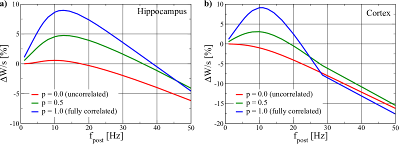
Figure 10: Simulation results of the synaptic weight change induced by a one-second train of spikes with different degrees of correlation, as a function of the frequency $f=f_{pre}=f_{post}$. The fraction $p$ of correlated spikes takes the values $0$, $0.5$, and $1$ in these plots. The delay between pre- and postsynaptic spikes was taken to be $5\mathrm{ms}$ in these simulations. The case $p=0$ corresponds to the dashed lines in Figs. 8 and 9. a) The pairwise hippocampal parameters (13) were used, together with $y_{c}=0.28$, $y_{b}=0.66$, and $x_{b}=0.62$, corresponding to the triplet fit. b) Here the pairwise cortical parameters (14) were used, together with $y_{c}=11.6$, $y_{b}=10.9$, and $x_{b}=0.5$, corresponding to the triplet fit.

 

We observe in Fig. 10, both for hippocampal and cortical neurons, that correlated spike trains induce an increasing amount of potentiation for low to intermediate frequencies ($\sim 1-10\mathrm{Hz}$). In the correlated scenario, and since in this case we are simulating a driving synapse, postsynaptic spikes follow presynaptic spikes in a causal order. When the frequency is higher than $10\mathrm{Hz}$, the interspike period becomes comparable to the STDP time window and each postsynaptic spike will also ”see” the following presynaptic spike, thus triggering the LTD term. Depending on the trace saturation constants, LTD or LTP will eventually dominate for large frequencies. If LTD dominates, depression results and after a certain reversal frequency the behavior is switched from Hebbian to Anti-Hebbian. This is the case for the triplet fitted values presented in Fig. 10.

It is important to note that the model is also able to produce Hebbian behavior within the entire physiological range of activities by changing $y_{c}$. The smaller the saturation effects are, the larger this reversal frequency becomes. In fact, with the second set of parameters used in Fig. 8 b), no such reversal is found within physiological frequencies (not shown here).

If observed, such a reversal, which is yet another side of the suppression effect, would have the benefit of being self-stabilizing, tuning synaptic strength to help keep neural activities bound.

The kink observable for the fully correlated curve ($p=1.0$) of 10 b) results from the particularly strong suppression effects in cortical neurons, captured in our model by $y_{b}<y_{c}$. For frequencies above a certain threshold ($\sim 28\mathrm{Hz}$) the trace concentration $y$ is always below the $y_{c}$ and LTP never triggers.

A fundamental difference between plots a) and b) is the different qualitative behavior between correlated and uncorrelated spikes. While in hippocampal neurons, Hebbian, increasing potentiation, is always present for low to intermediate frequencies (whether the spikes are correlated or not), in cortical neurons, our model predicts uncorrelated spikes always produce depression and therefor Hebbian learning requires the neurons to be at least partially correlated.

6 Comparison to other models

The problem of formulating plasticity in terms of the specific timing of pre- and postsynaptic spikes can be approached at different levels of detail and accuracy, ranging from simplistic phenomenological rules to detailed and complex models describing the different steps of the biological machinery responsible for STDP. In sections 3 and 4 the comparison of our model to simple forms of phenomenological rules has already been established, noting that linear combinations of spike pairs are generically not sufficient to explain the experimentally observed triplet non-linearities.

We have also shown that, while linear combinations of pairs, plus additional suppression, is enough to explain the triplet nonlinearities of cortical neurons, as shown in Froemke et al. (2002), hippocampal triplet non-linearities cannot be explained by suppression and a trace accumulation mechanism seems to be taking place in these synapses. In any case, this kind of phenomenological rules are not likely to generalize well to arbitrary spike patterns since no information of the underlying plasticity mechanism is present in the formulation.

Other models, like Albers et al. (2013) and Pfister et al. (2006), present interesting dynamical formulations of plasticity in terms of generic decaying markers or traces, but do not attempt to establish a link to the biological underpinnings of STDP. Calcium concentration and NMDA receptors have been shown to play a central role in time-dependent LTP and LTD, and we therefore believe it is important to formulate plasticity in those terms. Our model, though simplified, is formulated in terms of these key ingredients and may therefore help to bridge the worlds of functional and realistic models.

An alternative approach has been proposed by Appleby et al. (2007), where plasticity is described in an ensemble-based formulation. The authors there argue that the observed synaptic changes produced by standard protocols cannot be explained at a single synapse level, but rather state that the observed results arise at a population level. The authors then show how the pairwise STDP curve can be recovered at the ensemble level from all or nothing potentiation or depression at the single synapse level. The dependency of the model to the specific timing of triplets is however in this case not computed.

The model we present in this work belongs to the family of calcium-based spiking-neuron models. Within this family, models formulating synaptic plasticity exclusively in terms of the calcium levels (Uramoto et al., 2013; Graupner et al., 2012), while tuned to reproduce a variety of experimental results, tend to show paradoxical results when tested in other setups. The model presented by Uramoto et al. (2013), for example, predicts synaptic changes even when only postsynaptic spikes are present. The model in Graupner et al. (2012), in turn, shows plasticity also when either pre- or postsynaptic spikes are absent, since both pre- and postsynaptic spikes contribute directly to the calcium level in this model, without the need of coincidence. To avoid this, in our model we demand the simultaneous presence of both pre- and postsynaptic spikes for plasticity to arise, being proportional to the products of traces $x$ and $y$ in our rule. We believe this to be an important feature for simulations in situations of complex spike patterns where the pre- and postsynaptic firing rates do not necessarily match.

7 Discussion

We propose a basic trace model for timing-dependent plasticity that incorporates, in a first order approximation, the fundamental mechanisms acknowledged to be taking place in STDP. We show that the model successfully captures several main features of time-dependent plasticity, including the standard shape for low frequency pairing, experimentally observed triplet nonlinearities, and large frequency effects.

The decay constants for the two traces and the relative intensities of LTP and LTD can be extracted directly from the standard STDP curves, as measured for isolated pairs. The model is left hereafter with only three further parameters, which can be used to fit higher order contributions to plasticity. The model successfully reproduces the distinct and contrasting nonlinearities found in both hippocampal cultures and cortical slices.

While the model predicts a similar frequency dependence for correlated (or partially correlated) pre- and postsynaptic spikes both for hippocampal and cortical neurons, the effect of uncorrelated spikes (although smaller) differs qualitatively in these two types of neurons. In this case, the sign of the resulting plasticity depends for lower frequencies on the overall area of the pairwise STDP curve, resulting in potentiation for hippocampal neurons and depression in cortical ones, and for higher frequencies on the balance between spike suppression and trace accumulation.

We show that the model is able to reproduce typical frequency-dependencies for uncorrelated spikes, while fitting pairwise and triplet hippocampal parameters. We do also find, that fitting triplet results for L2/3 cortical neurons invariably leads to depression, for higher frequencies and of uncorrelated spikes, contrary to observations in L5 neurons. The question then arises, to which extent plasticity results for different neurons, or performed under different stimulation conditions, can be expected to match. It seems then essential to have available a consistent sets of experiments where pairwise, triplet, and frequency results are measured for the same type of neuron and with the same stimulation protocol. Otherwise one runs the risk of possibly trying to build a complete picture out of mismatching parts. In this sense, we hope that our predictions serve as a motivation to revisit and to complete triplet and frequency dependent studies for different types of neurons.

In order to compare our results with rate encoding plasticity models, we have also shown, by setting the presynaptic frequency to a constant value, that the amount of synaptic change is proportional, for hippocampal neurons, to the product of the activities, with a threshold that depends on the presynaptic firing rate. While the system lacks a longer term average threshold, as the one present in BCM, the presynaptic activity acts as a value of reference for the significant level of activity. If the postsynaptic activity exceeds this level then potentiation occurs, otherwise, depression arises.

For correlated spikes, we have shown that the model leads to similar results for hippocampal and cortical neurons, with an initial hebbian behavior for small to medium frequencies and, depending on choice for the parameters, a reversal to anti-hebbian behavior for large frequencies, which could have the virtue of being self-limiting, avoiding runaway growth of synaptic connections. It has been shown recently (Echeveste et al., 2014), that this self-limitation results naturally, for rate encoding neurons, from the stationarity principle for Hebbian learning. By tuning the value of $y_{c}$, the reversal frequency can be made larger, to the point of producing Hebbian behavior within the entire physiological range of activities.

The simplicity of the here proposed model makes it a useful tool for simulations and studies of the dynamical properties of networks adapted via these rules. Firstly, the calculations required are straightforward, making it computing time efficient. The relative small number of free parameters and their direct link to both the biophysical properties of the postsynaptic complex and to the dynamical features of the trace dynamics makes it suitable when studying the interplay between neural and synaptic dynamics in neural systems.

Appendix: Dimensionality Analysis

In section 2 we could have started by initially denoting by $x^{\prime}$ and $y^{\prime}$ the fraction of NMDA receptors and the $Ca^{2+}$ concentration, respectively, where the time evolution of these traces is written as:

$$\left\{\begin{array}[]{lcl}\dot{x}^{\prime}=-\frac{x^{\prime}}{\tau_{x}}+c_{1}\mathit{E_{x}}\sum_{\sigma}\delta(t-t_{pre}^{\sigma})\\ \dot{y}^{\prime}=-\frac{y^{\prime}}{\tau_{y}}+(c_{2}x^{\prime}+y^{\prime}_{c})\mathit{E_{y}}\sum_{\sigma}\delta(t-t_{post}^{\sigma})\end{array}\right.$$ (16)

where $\tau_{y}$ and $\tau_{x}$ represent the time constants in the decay of $x^{\prime}$ and $y^{\prime}$, and now two additional parameters $c_{1}$ and $c_{2}$ are included. $c_{1}$ represents the increase in $x^{\prime}$ caused by a single presynaptic spike (which in this simplified model we assume constant) and $c_{2}$ represents the increase, per unit of $x^{\prime}$, in $y^{\prime}$ concentration. $y^{\prime}_{c}$ is the constant contribution per postsynaptic spike to $y^{\prime}$ of the voltage-gated $Ca^{2+}$ channels. Again a spike efficacy $\mathit{E}$ is included that limits trace concentrations, where $\mathit{E}$ is still calculated as in (2).

Now, by a change of variables:

$$x=x^{\prime}/c_{1},\qquad x_{b}=x^{\prime}_{b}/c_{1},\qquad y=y^{\prime}/c_{1}c_{2},\qquad y_{c}=y^{\prime}_{c}/c_{1}c_{2},\qquad y_{b}=y^{\prime}_{b}/c_{1}c_{2}$$ (17)

we re-write (16) as:

$$\left\{\begin{array}[]{lcl}\dot{x}=-\frac{x}{\tau_{x}}+\mathit{E_{x}}\sum_{\sigma}\delta(t-t_{pre}^{\sigma})\\ \dot{y}=-\frac{y}{\tau_{y}}+(x+y_{c})\mathit{E_{y}}\sum_{\sigma}\delta(t-t_{post}^{\sigma})\end{array}\right.$$

which is the exactly the expression presented in section 2. By this procedure we have reduced the number of parameters for the trace evolution to 5.

References

- (1)
- Karmarkar et al. (2002) Karmarkar, U.R., & Buonomano, D.V. (2002). A model of spike-timing dependent plasticity: one or two coincidence detectors? J. Neurophysiol., 88, 507 – 513.
- Badoual et al. (2006) Badoual, M., Zou Q., Davison, A.P., Rudolph, M., Bal, T., Fregnac, Y., et al. (2006). Biophysical and phenomenological models of multiple spike interactions in spike-timing dependent plasticity. Int. J. Neural Systems, 16, (2), 79 – 97.
- Shouval et al. (2002) Shouval, H.Z., Bear, M.F., & Cooper, L.N. (2002). A unified model of NMDA receptor-dependent bidirectional synaptic plasticity. PNAS, 99, 10831 – 10836.
- Rubin et al. (2005) Rubin, J.E., Gerkin, R.C., Bi, G.Q., & Chow, C.C. (2005). Calcium time course as a signal for spike-timing-dependent plasticity. J. Neurophysiol., 96, 2600 – 2613.
- Graupner et al. (2012) Graupner, M., & Brunel, N. (2012). Calcium-based plasticity model explains sensitivity of synaptic changes to spike pattern, rate, and dendritic location. PNAS, 109, 3991 – 3996.
- Uramoto et al. (2013) Uramoto, T., & Torikai, H. (2013). A Calcium-Based Simple Model of Multiple Spike Interactions in Spike-Timing-Dependent Plasticity. Neural Computation, 25, 1853 – 1869.
- Malenka et al. (1999) Malenka, R.C., & Nicoll, R.A. (1999). Long-Term Potentiation - A Decade of Progress? Science, 285, 1870 – 1874.
- Bi et al. (2005) Bi, G.Q., & Rubin, J. (2005). Timing in synaptic plasticity: from detection to integration. Trends Neurosci., 28, 222 – 228.
- Meldrum (2000) Meldrum, B. S. (2000). Glutamate as a neurotransmitter in the brain: review of physiology and pathology. The Journal of nutrition., 130, 1007S – 1015S.
- Mayer et al. (1984) Mayer, M. L., Westbrook, G. L., & Guthrie, P. B. (1984). Voltage-dependent block by Mg2+ of NMDA responses in spinal cord neurones. Nature., 309, 261 – 263.
- Huang et al. (2004) Huang, Y. H., & Bergles, D. E. (2004). Glutamate transporters bring competition to the synapse. Current opinion in neurobiology, 14, 346 – 352.
- Carafoli (1987) Carafoli, E. (1987). Intracellular calcium homeostasis. Annual review of biochemistry., 56, 395 – 433.
- Colbran (2004) Colbran, R.J. (2004). Protein phosphatase and calcium/calmodulin-dependent protein kinase II-dependent synaptic plasticity. J. Neurosci., 24, 8404 – 8409.
- Cormier et al. (2001) Cormier, R.J., Greenwood, A.C., & Connor, J.A. (2001). Bidirectional synaptic plasticity correlated with the magnitude of dendritic calcium transients above a threshold. J. Neurophysiol., 85, 399 – 406.
- Neveu et al. (1996) Neveu, D., & Zucker, R.S. (1996). Title for the second reference. Postsynaptic levels of [Ca2+]i needed to trigger LTD and LTP, 16, 619 – 629.
- Yang et al. (1999) Yang, S.N., Tang, Y.G., & Zucker, R.S. (1999). Selective induction of LTP and LTD by postsynaptic [Ca2+]i elevation. J. Neurophysiol., 81, 781 – 787.
- Huang et al. (1992) Huang, Y., Colino, A., Selig, D.K., & Malenka, R.C. (1992). The Influence of Prior Synaptic Activity on the Induction of Long-Term Potentiation. Science, 225, 730 – 733.
- Bi et al. (1998) Bi, G.Q., & Poo, M.M. (1998). Synaptic Modifications in Cultured Hippocampal Neurons: Dependence on Spike Timing, Synaptic Strength, and Postsynaptic Cell Type. J. Neurosci., 18, 10464 – 10472.
- Bi (2002) Bi, G.Q. (2002). Spatiotemporal specificity of synaptic plasticity: cellular rules and mechanisms. Biol. Cybern., 87, 319 – 332.
- Hao et al. (2012) Hao, J., & Oertner, T. G. (2012) Depolarization gates spine calcium transients and spike-timing-dependent potentiation Current opinion in neurobiology, 22(3), 509 – 515.
- Froemke et al. (2002) Froemke, R.C., & Dan, Y. (2002). Spike-timing-dependent synaptic modification induced by natural spike trains. Nature, 146, 433 – 438.
- Nishiyama et al. (2000) Nishiyama, M., Hong, K., Mikoshiba, K., Poo, M. M., & Kato, K. (2000). Calcium stores regulate the polarity and input specificity of synaptic modification. Nature, 408(6812), 584 – 588.
- Turrigiano et al. (1994) Turrigiano, G., Abbott, L. F., & Marder, E. (1994). Activity-dependent changes in the intrinsic properties of cultured neurons. Science, 264, 974 – 976.
- Turrigiano et al. (1998) Turrigiano, G. G., Leslie, K. R., Desai, N. S., Rutherford, L. C., & Nelson, S. B. (1998). Activity-dependent scaling of quantal amplitude in neocortical neurons. Nature, 264, 892 – 896.
- Vitureira et al. (2013) Vitureira, N., & Goda, Y. (2013). The interplay between Hebbian and homeostatic synaptic plasticity. The Journal of cell biology, 203, 175 – 186.
- Sjöström et al. (2001) Sjöström, P.J., Turrigiano, G.G., & Nelson, S.B. (2001). Rate, timing, and cooperativity jointly determine cortical synaptic plasticity. Neuron, 32, 1149 – 1164.
- Wang et al. (2005) Wang, H.X. Gerkin, R.C., Nauen, D.W, & Bi, G.Q. (2005). Coactivation and timing-dependent integration of synaptic potentiation and depression. Nat. Neurosci., 8, 87 – 193.
- Bienenstock et al. (1982) Bienenstock, E. L., Cooper, L. N., & Munro, P. W. (1982). Theory for the development of neuron selectivity: orientation specificity and binocular interaction in visual cortex. The Journal of Neuroscience, 2, 32 – 48.
- Triesch (2007) Triesch, J. (2007). Synergies between intrinsic and synaptic plasticity mechanisms. Neur. Comp., 19, 885 – 909.
- Marković et al. (2012) Marković, D., & Gros, C. (2012). Intrinsic adaptation in autonomous recurrent neural networks. Neur. Comp., 24, 523 – 540.
- Linkerhand et al. (2013) Linkerhand, C., & Gros, C. (2013). Self-organized stochastic tipping in slow-fast dynamical systems. Mathematics and Mechanics of Complex Systems, 1, 129 – 147.
- Feldman (2000) Feldman, D.E. (2000). Timing-Based LTP and LTD at vertical inputs to Layer II/III pyramidal cells in rat barrel cortex. Neuron, 27, 45 – 56.
- Trachtenberg et al. (2000) Trachtenberg, J. T., Trepel, C., & Stryker, M. P. (2000). Rapid extragranular plasticity in the absence of thalamocortical plasticity in the developing primary visual cortex. Science, 287, 2029 – 2032.
- Albers et al. (2013) Albers, C., Schmiedt, J. T., & Pawelzik, K. R. (2013). Theta-specific susceptibility in a model of adaptive synaptic plasticity. Frontiers in computational neuroscience, 7.
- Pfister et al. (2006) Pfister, J. P., & Gerstner, W. (2006). Triplets of spikes in a model of spike timing-dependent plasticity. The Journal of neuroscience, 26(38), 9673 – 9682.
- Appleby et al. (2007) Appleby, P. A., & Elliott, T. (2007). Multispike interactions in a stochastic model of spike-timing-dependent plasticity. Neural computation, 19(5), 1362 – 1399.
- Linden et al. (2009) Linden, M. L., Heynen, A. J., Haslinger, R. H., & Bear, M. F. (2009). Thalamic activity that drives visual cortical plasticity. Nature neuroscience, 12(4), 390 – 392.
- Izhikevich et al. (2003) Izhikevich, E. M., & Desai, N. S. (2003). Relating stdp to bcm. Neural computation, 15(7), 1511 – 1523.
- Echeveste et al. (2014) Echeveste, G., & Gros, C. (2014). Generating functionals for computational intelligence: the Fisher information as an objective function for self-limiting Hebbian learning rules. Frontiers in Robotics and AI, 1, 1.