Spontaneous polarization in an interfacial growth model for actin filament networks with a rigorous mechano-chemical coupling

Abstract

Many processes in eukaryotic cells, including cell motility, rely on the growth of branched actin networks from surfaces. Despite its central role the mechano-chemical coupling mechanisms which guide the growth process are poorly understood, and a general continuum description combining growth and mechanics is lacking. We develop a theory that bridges the gap between mesoscale and continuum limit and propose a general framework providing the evolution law of actin networks growing under stress. This formulation opens an area for the systematic study of actin dynamics in arbitrary geometries. Our framework predicts a morphological instability of actin growth on a rigid sphere, leading to a spontaneous polarization of the network with a mode selection corresponding to a comet, as reported experimentally. We show that the mechanics of the contact between the network and the surface plays a crucial role, in that it determines directly the existence of the instability. We extract scaling laws relating growth dynamics and network properties offering basic perspectives for new experiments on growing actin networks.

I Introduction

Cells often migrate in response to external signals, including chemical and mechanical signals. Thereby the interfacial growth of filamentous actin polymer networks plays an important role Svitkina and Borisy (1999); Loisel et al. (1999). For example, cell crawling on a two-dimensional substrate involves the formation of a cytoplasmic membrane protrusion pointing in the direction of motion. Thereby, the necessary force for extending the membrane is provided by the polymerization of actin, a process far from chemical equilibrium, which converts chemical into mechanical energy. The same molecular machinery is also responsible for the propulsion of cellular organelles Taunton et al. (2000), pathogens Yarar et al. (1999); Cudmore et al. (1995) or biomimetic objects, such as spherical beads van Oudenaarden and Theriot (1999); Noireaux et al. (2000); Bernheim-Groswasser et al. (2002); van der Gucht et al. (2005); Delatour et al. (2008); Achard et al. (2010), vesicles Upadhyaya et al. (2003); Giardini et al. (2003); Delatour et al. (2008), droplets Boukellal et al. (2004), and ellipsoids Lacayo et al. (2012). In contrast, cell motion in a three-dimensional substrate is rather driven by blebbing, which relies on the contraction of the actin cortex by myosin motors to form protrusions Charras and Paluch (2008).

On the time scale of actin filament growth ($\sim 1\,$s) actin networks behave as nonlinear elastic solids Gardel et al. (2004); Janmey et al. (2007). Typically, the linear elastic modulus of actin networks formed during the propulsion of pathogens or biomimetic objects is in the range of 1 to 10 kPa Gerbal et al. (2000); Pujol et al. (2012). This raises the question of the coupling mechanism between growth dynamics and deformations (or stresses) in the network, a property which is often either neglected Dayel et al. (2009); Oelz et al. (2008); Kawska et al. (2012) or included via ad hoc assumptions, which do not necessarily respect all symmetries in the system Sekimoto et al. (2004); van der Gucht et al. (2005). Our objective is therefore to derive macroscopic evolution equations of actin networks combining a macroscopic constitutive law for its mechanical behavior and the actin polymerization kinetics in a rigorous way. The general formulation we present can be adapted to diverse situations relevant for actin dynamics. As a proof of principle we treat here the case of an elastic actin network growing from a spherical surface, where a spontaneous symmetry-breaking and the onset of motion has been observed experimentally van Oudenaarden and Theriot (1999); Noireaux et al. (2000); Bernheim-Groswasser et al. (2002); van der Gucht et al. (2005); Delatour et al. (2008); Achard et al. (2010).

To briefly outline the experimental observations (more details can be found in Blanchoin et al. (2014)), actin polymerizes on the surface of a sphere with a radius of about 1 $\mu$m into a cross-linked/entangled network, which forms initially a closed spherical shell. Growth and cross-linking is restricted to a zone close to the surface of the sphere. Monomers diffuse freely through the network to reach the growth zone and are inserted between the already existing network and the sphere, which leads to a relative motion between older network layers and the surface and to the buildup of mechanical stresses. Eventually the actin shell undergoes a spontaneous symmetry-breaking, leading to the formation of an actin tail. Two mechanisms for symmetry-breaking have been proposed: (i) the external actin shell ruptures at one point due to elongational stresses van der Gucht et al. (2005), or (ii) the instability is due to actin polymerizing slower on one side of the surface than on the other side Delatour et al. (2008).

Our understanding of these processes has been advanced through several theoretical studies based on discrete models on the scale of the filament van Oudenaarden and Theriot (1999); Mogilner and Oster (2003), mesoscopic models Dayel et al. (2009); Oelz et al. (2008); Kawska et al. (2012) or phenomenological continuous models Sekimoto et al. (2004); Lee et al. (2005); van der Gucht et al. (2005); John et al. (2008). Rather surprisingly, a general growth law based on first thermodynamic principles which links the stresses in the network (which depend on the growth history itself and the relevant boundary conditions) to the interface dynamics is lacking. Our approach closes this gap. In this brief exposition, we exploit the framework to show that an instability arises from the interplay between interfacial growth kinetics and mechanical stresses, which reflect the growth history of the network. Thereby the nature of the contact formed between the network and the bead surface (fixed vs. sliding) is crucial in the overall macroscopic dynamics. In a spherical geometry a spontaneous polarization into front and back is possible when the filaments can slide on the surface, but not when they are fixed to the surface. Furthermore we derive scaling laws for the instability characteristics which form a consistent picture with experiments.

The problem of symmetry-breaking has been studied theoretically on the continuum level in Sekimoto et al. (2004); John et al. (2008). However, in contrast to Sekimoto et al. (2004); John et al. (2008) we describe here the buildup of stresses and strains in the network due to growth and the subsequent mechano-chemical coupling in a rigorous way, consistent with a hyperelastic macroscopic constitutive law of the network. For example, the model in Sekimoto et al. (2004) tacitly assumes a vanishing Poisson ratio and the stress distribution can only be solved consistently in an axisymmetric or spherical configuration. The model in John et al. (2008) is limited to small deformations arising from a small displacment at the internal bead/network interface. Moreover, our description distinguishes between reference and deformed network configurations, which is essential for describing a growing interface in contact with a solid stationary substrate (the spherical surface), where the growth process manifests itself as a displacement of a free interface (in contact with the solvent). This crucial distinction between reference and deformed frame is absent in Sekimoto et al. (2004); John et al. (2008) and limits their predictive power.

II Model

II.1 Mechanical description of the network

Recently we have proposed a macroscopic mechanical model of actin networks starting from a microscopic description and have shown that it captures the basic bulk rheological properties of actin networks John et al. (2013). A major issue is now, how to properly combine interfacial growth and mechanics. We first briefly recall the description of the network mechanics and then introduce the dynamical equations for the interfaces. For simplicity, we consider a 2D geometry (albeit a 3D study does not pose a specific challenge, but increases the technical complexity).

We assume a structurally periodic planar filament network with the topology shown in Fig. 1, which is in contact with the surface of a cylinder of radius $R_{0}$. The typical scale of the elementary cell $l_{0}$ is small compared to a macroscopic scale $R_{0}$, which introduces the small parameter $\eta=l_{0}/R_{0}\ll 1$.

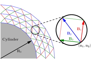
Figure 1: Sketch of a small part of the filament network showing the different types of elementary vectors $\mathbf{B}_{i}$ of one elementary cell labeled $(n_{1},n_{2})$ in different colors.

Each elementary cell contains one node, identified by a doublet of integers $(n_{1},n_{2})$, and three filaments, described by the vectors $\mathbf{B}_{i}$ with $i=1,2,3$. It has a quadrilateral shape with the filaments $\mathbf{B}_{1}$ and $\mathbf{B}_{3}$ forming the sides and the filament $\mathbf{B}_{2}$ forming a diagonal. A node is formed by the intersection of six filaments, three of which belong to the same elementary cell as the node, the other three belonging to neighboring elementary cells. For example, the node ($n_{1},n_{2}$) shown in Fig. 1 connects the filaments $\mathbf{B}_{1}$, $\mathbf{B}_{2}$, and $\mathbf{B}_{3}$ of the same node with the filaments $\mathbf{B}_{1}$ from node ($n_{1}-1,n_{2}$), $\mathbf{B}_{2}$ from node ($n_{1},n_{2}-1$) and $\mathbf{B}_{3}$ from node ($n_{1}+1,n_{2}-1$). This network topology is one of the most simple topologies. Other structures involving several nodes per elementary cell are possible. However, the resulting mechanical equilibrium equations are much more involved, than for simple structures with only one node per elementary cell.

In a simple picture the filaments behave as entropic springs Gardel et al. (2004) and the elastic energy of the filament $\mathbf{B}_{i}$ is given by a harmonic potential

$$f_{i}={k\over 2l_{0}}(l_{i}-l_{0})^{2}$$ (1)

with the equilibrium strand length $l_{0}$ and the actual strand length $l_{i}=|\mathbf{B}_{i}|=\sqrt{\mathbf{B}_{i}\cdot\mathbf{B}_{i}}$. We find it a bit more convenient to rewrite (1) in a different way which is valid as long as the actual length $l_{i}$ is close to $l_{0}$. Indeed, in this case, since $(l_{i}^{2}-l_{0}^{2})^{2}\simeq 4l_{0}^{2}(l_{i}-l_{0})^{2}$, we can write

$$f={k\over 8l_{0}^{3}}\sum_{i}^{3}\left(l_{i}^{2}-l_{0}^{2}\right)^{2}.$$ (2)

Once the microscopic model is introduced, we can now write the macroscopic equation. Owing to the fact that $\eta=l_{0}/R_{0}\ll 1$ one introduces a set of continuous variables $(\lambda_{1},\lambda_{2})$ John et al. (2013), such that the node positions are approximated by a continuous vector function $\boldsymbol{\phi}(\lambda_{1},\lambda_{2})$ and the filament vectors $\mathbf{B}_{i}$ are given by Taylor expansions of $\boldsymbol{\phi}$ up to $\mathcal{O}(\eta)$

$$\mathbf{B}_{1,3}=\pm\mathbf{h}_{1}+{1\over 2}\mathbf{h}_{2}\quad\mbox{and}\quad\mathbf{B}_{2}=\mathbf{h}_{2},\quad\mbox{with}\quad\mathbf{h}_{i}=\eta\partial_{\lambda_{i}}\boldsymbol{\phi}.$$ (3)

The surface in contact with the cylinder is called ”inner interface” as opposed to the “outer interface” in contact with the solvent. In the axisymmetric situation $\lambda_{1}\in(0,\Lambda_{1})$ and $\lambda_{2}\in(0,2\pi)$ correspond to the radial and angular directions, respectively. The unit vector in the radial direction is given by $\mathbf{\hat{r}}=\cos{(\lambda_{2})}\mathbf{\hat{x}}+\sin{(\lambda_{2})}\mathbf{\hat{y}}$. Consequenlty, the vectors $\mathbf{h}_{1}$ and $\mathbf{h}_{2}$ point into the radial and angular directions, respectively.

In the continuum limit the discrete sum of (2) over all nodes can be converted into an integral over the continuous variables in the domain $\Omega$ occupied by network, so that the total network energy reads

$$F[\boldsymbol{\phi}]={1\over\eta^{2}}\int_{\Omega}f(\boldsymbol{\phi})\,d\lambda_{1}\,d\lambda_{2},$$ (4)

where by using (2) and (3), $f$ can be expressed only in terms of the continuous function $\boldsymbol{\phi}$. Since growth occurs on a slow time scale, as compared to the propagation of sound in the actin network, the system can be viewed at each instant at mechanical equilibrium, which corresponds to a minimum of $F$ with respect to a variation of $\boldsymbol{\phi}$. This yields $0=\partial_{\lambda_{1}}\mathbf{T}_{1}+\partial_{\lambda_{2}}\mathbf{T}_{2}$ (divergence-free stress, as in classical linear elasticity). The stress is defined as $\mathbf{T}_{i}=\partial f/\partial\mathbf{h}_{i}$ (the two components of the vectors $\mathbf{T}_{i}$ define the stress tensor). The $\mathbf{T}_{i}$ are explicitely given by

$$\mathbf{T}_{1} = {k\over l_{0}^{3}}\left[(l_{1}^{2}-l_{0}^{2})\mathbf{B}_{1}-(l_{3}^{2}-l_{0}^{2})\mathbf{B}_{3}\right]$$ (5)

$$\mathbf{T}_{2} = {k\over l_{0}^{3}}\left[{(l_{1}^{2}-l_{0}^{2})\over 2}\mathbf{B}_{1}+(l_{2}^{2}-l_{0}^{2})\mathbf{B}_{2}+{(l_{3}^{2}-l_{0}^{2})\over 2}\mathbf{B}_{3}\right].$$ (6)

and define the constitutive law (relation between stress and strain). Physically, the vector $\mathbf{T}_{1}$ ($\mathbf{T}_{2}$) denotes the force exerted on a facet oriented in the direction $\mathbf{h}_{2}$ ($\mathbf{h}_{1}$) with length $|\mathbf{h}_{2}|$ ($|\mathbf{h}_{1}|$). The associated boundary conditions are

$$|\boldsymbol{\phi}| = R_{0}\quad\mbox{and}\quad\mathbf{T}\cdot\mathbf{t}=0\quad\mbox{at the inner inteface}$$ (7)

$$\mathbf{T} = 0\quad\mbox{at the outer interface}$$ (8)

where $\mathbf{T}$ and $\mathbf{t}$ denote the traction force and the tangent vector at the interface. (7) is equivalent to a shear free inner interface (where actin filament nucleators are present) which is everywhere in contact with the cylinder surface and (8) is equivalent to a force free outer interface.

It has been shown John et al. (2013) that the potential energy per node $f$ [Eq. (2)] is equivalent to the strain energy density of an isotropic St.-Venant-Kirchhoff hyperelastic solid with the Lamé coefficients $\lambda=\mu=\sqrt{3}k/(4l_{0})$, the Young’s modulus $Y=2k/(\sqrt{3}l_{0})$ and the Poisson ratio $\sigma=1/3$. This constitutive law results in a strain stiffening and negative normal forces under a simple volume conserving shear, a typical behavior observed experimentally for semiflexible networks Gardel et al. (2004); Janmey et al. (2007).

II.2 Growth kinetics and interface dynamics

The main issue that remains to be addressed, is how one could link mechanics with actin growth dynamics in a consistent way, and what are the far-reaching consequences. For simplicity, we consider the case that the network grows at the inner interface. That is, the topology of the network remains unchanged while adding or subtracting an elementary material element at the interface. The cost in energy by adding (subtracting) a material element will define the chemical potential difference $\Delta\mu$ that drives the interface using the following kinetics relating the normal velocity $v_{n}$ to the chemical potential balance

$$v_{n}=-M\Delta\mu=-M(\Delta\mu_{c}+\Delta\mu_{m})\,.$$ (9)

$M$ is a positive mobility constant. $\Delta\mu$ is composed of an attachment part $\Delta\mu_{c}$ due to chemical bond formation (we assume it to be a constant) and an elastic part $\Delta\mu_{m}={\partial F\over\partial\Omega}$, which is given by the functional derivative of the total strain energy $F$ (4) with respect to a change in the shape of the network by respecting the boundary conditions (7,8). We merely focus here on the main outcomes (details are in Appendix A). For the inner interface we find

$$\Delta\mu_{mi}={1\over\eta^{2}}\left[f-\mathbf{T}\cdot\mathbf{h}\right],$$ (10)

where $\mathbf{T}=\mathbf{T}_{i}\nu_{i}$ denotes the traction force at the interface with $\nu_{i}$ being the $ith$-component of the unit normal outward vector in the material frame $(\lambda_{1},\lambda_{2})$. $\mathbf{h}=\mathbf{h}_{i}\nu_{i}$ is a measure for the displacement of the old network interface due to the insertion of new material between the solid cylinder and the soft network. All quantities are calculated at the interface position where the material is added. Intuitively one can interpret Eq. (10) in the following way. The energy cost for inserting a material element at the internal boundary contains the straining of the material element to the same state as neighboring interfacial elements and also the work which is necessary to displace the old interface against the traction force to make room for the new material (the cylinder being rigid cannot be displaced). Expression (10) is the general form of the chemical potential difference at the internal interface, which is valid for any material whose constitutive law can be expressed in the form of Eqs. (5) and (6). At the force free external interface the elastic chemical potential is simply given by $\mu_{me}={1\over\eta^{2}}f$. Setting $\Delta\mu_{m}=\Delta\mu_{mi}$ and reporting (5) and (6) into (10) leads to a nonlinear evolution equation (9) relating growth speed and direction $v_{n}$ [Eq. (9)] to the configuration of the network $\boldsymbol{\phi}$. The resulting equation (9), together with (5,6) and boundary conditions (7,8) constitute the general framework that can be applied to any configuration and geometry. We treat here only the problem inspired by the actin comet formation on rigid beads.

III Results

Having defined the mechanical and dynamical equations in a consistent manner, we will now explore some consequences. We first consider the case of an axisymmetric state of the network and analyse then its linear stability with respect to a morphological perturbation.

III.1 Axisymmetric network

In the axisymmetric state the network geometry is described by the ”radial layer number” $\Lambda_{1}$. Recall that if in the discrete network the true number of nodes in the radial direction is $N_{1}$ (with $N_{1}$ being a large integer), in the continuum limit the relation $\Lambda_{1}=N_{1}\eta=N_{1}l_{0}/R_{0}$ holds. We look for an axisymmetric configuration of the form $\boldsymbol{\phi}=\phi_{R}\mathbf{\hat{r}}.$ Equations (2-8) are solved numerically using continuation methods Doedel et al. (1998).

Figure 2 (a) shows the observable thickness $h$ of the network $h=\phi_{R}(\Lambda_{1})-R_{0}$ in the mechanical equilibrium configuration depending on the radial layer number $\Lambda_{1}$. The distinction between the observable thickness and the radial layer number is important, since they are not necessarily related in a linear manner.

Figure 2: Observable network thickness $h$ depending on the radial layer number $\Lambda_{1}$.

For thin networks $h$ increases linearly with $\Lambda_{1}$ and one finds $h/R_{0}=\sqrt{3}\Lambda_{1}/2$. For larger networks the tangential tension at the outer network interface leads to a radial compression and $h$ nearly saturates for $\Lambda_{1}\simeq 0.8$. An interesting property follows naturally from our formulation, which is that for an axisymmetric state the elastic chemical potential difference is identical at the two interfaces, denoted as $\Delta\mu^{(0)}_{m}$. If the thickness of the network is modified, there is no way to discriminate between the fact that material has been exchanged at the cylinder surface or at the free surface, only the initial and the final thickness matter, and not the path followed by the system. This property is not only comforting the theory, but can even be exploited to extract some interesting results. Indeed, it is possible to determine analytically the chemical potential at the external surface, which is linked to the observable network thickness $h$ in a simple way (see Appendix A for details)

$$\Delta\mu_{m}^{(0)}={kh^{2}\over 8l_{0}R_{0}^{2}}\left(h+2R_{0}\right)^{2}\,,$$ (11)

where we have used the fact that the filaments of type 1 and 3 (cf. Fig. 1) are at equilibrium length [to ensure a vanishing traction force (8)] and the filaments of type 2 have length $l_{2}=l_{0}/R_{0}\phi_{R}(\Lambda_{1})=l_{0}(h+R_{0})/R_{0}$. Now we consider growth of an axisymmetric network whereby polymerization only occurs at the internal interface with $\Delta\mu_{c}<0$. Dendritic actin networks nucleated by the Arp2/3 complex typically show a kinetic polarity with a rapidly polymerizing ’plus’-end interface directed towards the nucleating surface i.e. $\Delta\mu_{ci}<0$, and a slowly depolymerizing ’minus’-end oriented towards the solvent, i.e. $\Delta\mu_{ce}>0$ Pollard et al. (2000). For more clarity we consider here only the case, that the motility medium does not contain any fragmentation proteins, such as cofilin and we treat the limiting case that growth only occurs at the internal interface while the external interface is stationary. The model can be straightforwardly extended to two dynamical interfaces, which gives for example the treadmilling behavior.

If growth occurs only at the internal interface the interface velocity (9) vanishes in steady state and one finds in the limit $h\ll 2R_{0}$ for the observable stationaray network thickness

$$\bar{h}=\sqrt{-{2l_{0}\Delta\mu_{c}\over k}},$$ (12)

where $\bar{h}$ stands for the steady thickness. Recall that in steady state the radial layer number is related to the observable thickness by $\bar{h}=\phi_{R}(\bar{\Lambda}_{1})-R_{0}$. Expression (12) can be further related to the network properties and geometry and to the known rate equations of actin polymerization, which offers interesting scaling relations, which will be discussed at the end of this Letter.

The next important step is to analyze the linear stability against modulations of the gel thickness.

III.2 Linear stability analysis

We introduce a small perturbation of amplitude $\varepsilon$ at the internal interface, while the structure of the external interface remains unchanged. The perturbation is encoded in the growth velocity at the internal surface. Since we consider a system, which is periodic (period $2\pi$) and translationally invariant in $\lambda_{2}$ a perturbation of any quantity (shape, strain, growth velocity) can be expressed in terms of a $\cos$-series with wavenumber $q$ and growth rate $\beta_{q}$. We have solved the model equations in the linear regime.

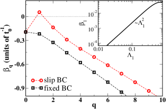
Figure 3: Dispersion relation for the shear-free (slip BC) and the Dirichlet (fixed BC) boundary condition. Parameters are $\bar{\Lambda}_{1}=0.7$. The time scale is $t_{0}=l_{0}/(MkR^{2}_{0})$. The inset shows the positive growth rate $\beta_{1}$ depending on the radial layer number $\Lambda_{1}$.

Figure 3 shows a typical dispersion relation. Also shown is the dispersion relation for an alternative boundary condition, that the network is fixed and cannot slide on the cylinder surface, i.e. condition (7) is replaced by $\boldsymbol{\phi}=R_{0}\mathbf{\hat{r}}$ at the internal interface. A robust and interesting outcome is that only perturbations with the wave number $q=1$ are unstable (i.e. $\beta_{1}>0$), while all other modes are stable. For relatively thin networks we find $\beta_{1}=MkR_{0}^{2}\bar{\Lambda}_{1}^{2}/l_{0}$. This instability is only present when the network can slide on the cylinder surface. When the bonds are fixed, no instability is found. The mode selection arises naturally within the model. Damping of high modes is naturally present in the model due to the accumulation of elastic shear-stresses in the bulk.

The instability corresponding to wave number $q=1$ means, that the network shrinks at one side of the cylinder and grows at the opposite side of the cylinder, i.e. the instability initiates the formation of an actin comet as observed in biomimetic motility experimentsvan Oudenaarden and Theriot (1999); van der Gucht et al. (2005); Achard et al. (2010); Upadhyaya et al. (2003); Giardini et al. (2003); Delatour et al. (2008); Boukellal et al. (2004).

a b

Figure 4: Network shape before (a) and after symmetry-breaking (b). (b) was obtained by superimposing the axisymmetric shape and the unstable mode with the amplitude $0.15\,\Lambda_{1}$. The color encodes the spatial distribution of the strain energy density (a) and the change in strain energy density (b). The energy density scale is $k/l_{0}$.

Figure 4 shows typical shapes of the network before and after symmetry-breaking. Also shown is the strain energy density [Fig. 4 (a)] and the change in strain energy density compared to the axisymmetric shape [Fig. 4 (b)]. Interestingly, the symmetry is broken by increasing the strain energy density in the thin network regions (front) and by decreasing it in the thick network regions (back). As time evolves the instability should be amplified and other mechanisms (e.g. fracture) may get important and lead to a larger comet. A detailed study of the subsequent nonlinear regime will be dealt with in the future.

III.3 Scaling properties and comparison with experiments

In the following we will discuss some scaling relations (see Appendix B for more details). We base our calculations on the assumptions, that the filaments behave as entropic springs with persistance length $l_{p}$ Gardel et al. (2004), and that free monomers (concentration $c$, size $l_{m}$) polymerize into linear filaments with the known kinetics $k_{+}(c-c_{c})$ in the absence of mechanical stress Pollard et al. (2000), where $k_{+}$ denotes the rate constant of polymerization and $c_{c}$ denotes the critical monomer concentration, at which the polymerization speed is zero. We find the following scaling for the observable stationary network thickness (12)

$$(\bar{h}/R_{0})^{2}\sim{l_{0}^{3}(c-c_{c})\over l_{p}^{2}l_{m}c_{c}}$$ (13)

Using typical values for $l_{0}=100\,$nm, $l_{p}=10\,\mu$m, $l_{m}=3\,$nm and $c/c_{c}=10$ we find ${\bar{h}/R_{0}}\sim 0.2$. This value and the linear scaling of $\bar{h}$ with $R_{0}$ are consistent with experiments van der Gucht et al. (2005). The growth rate scales as $\beta\sim k_{+}(c-c_{c})l_{m}/R_{0}$ which yields a time scale for the birth of the instability

$$\tau\sim{R_{0}\over l_{m}k_{+}(c-c_{c})}$$ (14)

Using $R_{0}=1\,\mu$m and $k_{+}(c-c_{c})=1\,$s^-1 Pollard et al. (2000) one finds a typical time $\tau=5\,$min, which is a reasonable value van der Gucht et al. (2005).

IV Discussion

We have provided a general theoretical framework for stress and actin growth coupling. Application to actin growth on beads led to the following major results: (i) the surprising mode selection $q=1$ and the stabilization of all higher modes without needing an ad-hoc cut-off length, (ii) the role of the boundary conditions at the nucleating surface (sliding/fixed) for the existence of the instability, (iii) the scaling laws which are consistent with experiments. The instability reported here is induced by growth and not by fracture. Experiments on vesicles Delatour et al. (2008) as a nucleating surface are consistent with this mechanism. They suggest, that for vesicles symmetry-breaking does not occur via a fracture mechanism at the external network interface, but via a variation in the growth speed along the internal vesicle/network interface. In Delatour et al. (2008) it was observed that shortly after symmetry-breaking the newly formed network layers at the internal interface had a varying thickness (thin on one side, thick on the opposite side of the vesicle), wereas older network layers at the external network interface maintained a homogeneous thickness. This observation is consistent with an asymmetric network polymerization at the internal interface. It is reasonable to expect bonds at the membrane to slide due to the fluid nature of the membrane, supporting our outcome that only in this case an instability takes place. For experiments with rigid beads van der Gucht et al. (2005) it is not obvious (albeit not excluded) that bonds can slide, but still an instability could be observed. It has been proposed by the authors van der Gucht et al. (2005) that the instability is triggered by fracture of the network. In preliminary calculations we have also identified a morphological instability of purely mechanical origin. However, this instability requires a critical network thickness, beyond the thickness which we considered here. A further investigation of this problem as well as other growth geometries (lamellipodium) and the effect of active stresses Kruse et al. (2004) will be part of future work.

Appendix A Derivation of the elastic chemical potential difference

In the derivation of the elastic chemcical potential we will assume a strain energy functional with the boundary conditions defined in Eqs. (2-8) in the main text. The elastic chemical potential difference $\Delta\mu_{m}$ for inserting a material element at the network interface can be calculated from the variation of the elastic strain energy $F$ with respect to a change in shape of the elastic body in the material frame $\Omega$ by respecting the prescribed boundary conditions

$$\Delta\mu_{m}={\delta F\over\delta\Omega}\,.$$ (15)

Upon a modification of $\Omega$ by $\delta\Omega$ the change in the strain energy is given to lowest order in $\delta\Omega$ by

$$\delta F={1\over\eta^{2}}\int_{\Omega}\mathbf{T}_{i}\cdot\delta\mathbf{h}_{i}\,d\lambda_{1}d\lambda_{2}+{1\over\eta^{2}}\int_{\delta\Omega}fd\lambda_{1}d\lambda_{2}$$ (16)

with $\mathbf{T}_{i}=\partial f/\partial\mathbf{h}_{i}$ and $\mathbf{h}_{i}=\eta\partial_{\lambda_{i}}\boldsymbol{\phi}$. Upon partial integration of (16) one finds

$$\delta F = -{1\over\eta}\int_{\Omega}\partial_{\lambda_{i}}\mathbf{T}_{i}\cdot\delta\boldsymbol{\phi}\,d\lambda_{1}d\,\lambda_{2}+{1\over\eta}\int_{S}\mathbf{T}\cdot\delta\boldsymbol{\phi}\,ds+$$ (17)

$${1\over\eta^{2}}\int_{\delta\Omega}fd\lambda_{1}d\lambda_{2}$$

with $\mathbf{T}=\mathbf{T}_{1}\nu_{1}+\mathbf{T}_{2}\nu_{2}$ and where $\nu_{1}$ and $\nu_{2}$ denote the components of the unit outward normal vector $\boldsymbol{\nu}$ in the material frame $(\lambda_{1},\lambda_{2})$.

The first integral in (17) vanishes due to the mechanical equilibrium condition $\partial_{\lambda_{i}}\mathbf{T_{i}}=0$ and only the second and third integral in (17) will contribute to the chemical potential difference. Now, we assume that the perturbation of the interface is described by a function $\epsilon(|s-s_{0}|)\boldsymbol{\nu}(s)$, with $\epsilon(|s-s_{0}|)\ll 1$. Since the perturbation of the boundary is local and $\epsilon$ is decaying rapidly with $|s-s_{0}|$ we can evaluate the third integral in (17) to the lowest order

$$\int_{\delta\Omega}f\,d\lambda_{1}\,d\lambda_{2}=\int_{S}f(s)\epsilon(|s-s_{0}|)\,ds=f(s_{0})\delta\Omega$$ (18)

The second integral over the boundary of the unperturbed domain depends crucially on the boundary condition. First we will consider the simple case of a material exchange at the external force-free interface with $\mathbf{T}=0$. In this case also the line integral in (17) vanishes and we find

$$\delta F={1\over\eta^{2}}f(s_{0})\delta\Omega,$$ (19)

which leads to the elastic chemical potential difference for a perturbation at $s_{0}$ at the external interface

$$\Delta\mu_{me}={1\over\eta^{2}}f(s_{0})$$ (20)

In the axisymmetric configuration (20) can be linked to the observable network thickness $h=\phi_{R}(\Lambda_{1})-R_{0}$ in a simple way. Making use of the fact that the traction vector $\mathbf{T}$ at the external interface vanishes for $l_{1}=l_{3}=l_{0}$ and since $l_{2}=\eta\phi(\Lambda_{1})=\eta(R_{0}+h)$, one finds after some manipulation of (20) one recovers Eq. (11) from the main text

$$\Delta\mu_{me}^{(0)}={kh^{2}\over 8l_{0}R_{0}^{2}}\left(h+2R_{0}\right)^{2}.$$ (21)

Next we consider the more complex case of a material exchange at the internal interface. Taking advantage of the boundary conditions [Eq. (7) in the main text] we note first that after a modification of the internal boundary we find for the position of the internal boundary up to lowest order in the perturbation

$$R_{0}^{2}=\boldsymbol{\phi}\cdot\boldsymbol{\phi}+2\boldsymbol{\phi}\cdot(\delta\boldsymbol{\phi}+\partial_{\lambda_{i}}\boldsymbol{\phi}\nu_{i}\epsilon).$$ (22)

The position of the boundary before the perturbation $\boldsymbol{\phi}$ fulfills $|\boldsymbol{\phi}|=R_{0}$ and it follows that

$$0=\boldsymbol{\phi}\cdot(\delta\boldsymbol{\phi}+\partial_{\lambda_{i}}\boldsymbol{\phi}\nu_{i}\epsilon)\quad\mbox{and}\quad\boldsymbol{\phi}\cdot\delta\boldsymbol{\phi}=-\boldsymbol{\phi}\cdot\partial_{\lambda_{i}}\boldsymbol{\phi}\nu_{i}\epsilon.$$ (23)

Since the vectors $\boldsymbol{\phi}$ and $\mathbf{T}$ are parallel to the normal direction of the boundary we can write using identity (23)

$$\mathbf{T}\cdot\delta\boldsymbol{\phi}={1\over R_{0}^{2}}(\mathbf{T}\cdot\boldsymbol{\phi})(\boldsymbol{\phi}\cdot\delta\boldsymbol{\phi})=-\mathbf{T}\cdot\partial_{\lambda_{i}}\boldsymbol{\phi}\nu_{i}\epsilon.$$ (24)

After an elementary manipulation we find from (17) and (18)

$$\delta F = -{1\over\eta^{2}}\int_{S}\mathbf{T}\cdot\mathbf{h}\ \epsilon(|s-s_{0}|)\,ds+{1\over\eta^{2}}f(s_{0})\delta\Omega$$ (25)

$$= {1\over\eta^{2}}\left[f-\mathbf{T}\cdot\mathbf{h}\right]_{0}\delta\Omega,$$

with $\mathbf{h}=\eta\partial_{\lambda_{i}}\boldsymbol{\phi}\nu_{i}$ and where the subscript ₀ indicates that all quantities are calculated at the position $s_{0}$. From (25) we infer the elastic chemical potential difference at the internal interface [Eq. (10) in the main text]

$$\Delta\mu_{mi}={1\over\eta^{2}}\left[f-\mathbf{T}\cdot\mathbf{h}\right].$$ (26)

Appendix B Scaling behavior

Here we demonstrate some scaling relations, relevant for biomimetic experiments on actin driven motility. First we note, that the polymerization part of the chemical potential $\Delta\mu_{c}$ used in Eq. (10) in the main text is based on a material exchange in Lagrangian coordinates. Therefore, the change in chemical potential per node is given by $\eta^{2}\Delta\mu_{c}$, which can be related to the chemical potential difference per monomer $\Delta\tilde{\mu}_{c}$ by assuming that each node contains 3 filaments of length $l_{0}$ and that each filament contains $l_{0}/l_{m}$ monomers of size $l_{m}$. Consequently

$$\Delta\tilde{\mu}_{c}={l_{0}l_{m}\over 3R_{0}^{2}}\Delta\mu_{c}=-k_{B}T\ln{c\over c_{c}}$$ (27)

where $c$ denotes the actual concentration of monomers in solution, $c_{c}$ denotes the critical monomer concentration where the polymerization speed vanishes and $k_{B}T$ denotes the thermal energy. Using expression (27) we can write

$$\left({\bar{h}\over R_{0}}\right)^{2}=-{2l_{0}\Delta\mu_{c}\over kR_{0}^{2}}={6k_{B}T\over kl_{m}}\ln{c\over c_{c}}$$ (28)

Assuming now, that the filaments behave as entropic springs with spring constant $k=k_{B}Tl_{p}^{2}/l_{0}^{3}$ Gardel et al. (2004), where $l_{p}$ denotes the persistence length we find

$$\left({\bar{h}\over R_{0}}\right)^{2}={6l_{0}^{3}\over l_{p}^{2}l_{m}}\ln{c\over c_{c}}\approx{6l_{0}^{3}\over l_{p}^{2}l_{m}c_{c}}(c-c_{c})$$ (29)

Note the linear scaling of $\bar{h}$ with $R_{0}$ as observed experimentally in van der Gucht et al. (2005). Using typical values for $l_{0}=100\,$nm, $l_{p}=10\,\mu$m, $l_{m}=3\,$nm and $c/c_{c}=10$ one finds $\bar{h}/R_{0}\approx 0.2$.

Now, we use the known kinetic eqation of polyerization of actin to estimate the time scale of symmetry breaking $t_{0}=l_{0}/(MkR_{0}^{2})$, i.e. we estimate the mobility constant $M$. Typically the polymerization of actin without mechanical stresses is described by the following kinetic equation Pollard et al. (2000)

$$v_{p}=k_{+}(c-c_{c})$$ (30)

where $k_{+}$ denotes the rate constant of polymerization. The normal interface velocity [Eq. (9) in the main text] is related to the polymerization speed by $v_{n}\approx l_{m}/R_{0}v_{p}$ and we find

$$v_{p} = {R_{0}\over l_{m}}v_{n}=-{R_{0}\over l_{m}}M\Delta\mu_{c}={3MR_{0}^{3}k_{B}T\over l_{0}l_{m}^{2}}\ln{c\over c_{c}}$$ (31)

$$= {3MR_{0}^{3}k_{B}T\over l_{0}l_{m}^{2}c_{c}}(c-c_{c})$$

Comparisson of (31) with (30) gives the following expression for the mobility constant

$$M={k_{+}c_{c}l_{0}l_{m}^{2}\over 3R_{0}^{3}k_{B}T}$$ (32)

and the time scale $t_{0}$ can be rewritten as

$$t_{0}={l_{0}\over MkR_{0}^{2}}={3R_{0}l_{0}^{3}\over k_{+}c_{c}l_{p}^{2}l_{m}^{2}}$$ (33)

As stated in the main text, the growth rate for symmetry-breaking scales as $\beta_{1}\sim\bar{\Lambda}^{2}/t_{0}$ for relatively thin networks. Assuming $\bar{\Lambda}_{1}^{2}\sim(\bar{h}/R_{0})^{2}$ and using (29) and (33) we find the following scaling $\beta_{1}\sim k_{+}(c-c_{c})l_{m}/R_{0}$. Consequently the typical time scale for symmetry-breaking scales linearly with $R_{0}$ as shown experimentally in van der Gucht et al. (2005). For $R_{0}=1\,\mu$m and $k_{+}(c-c_{c})=1$ $s^{-1}$ Pollard et al. (2000) one finds a typical time scale of symmetry-breaking of 5 min, which is a reasonable result van der Gucht et al. (2005).

References

- Svitkina and Borisy (1999) T. M. Svitkina and G. G. Borisy, J. Cell Biol. 145, 1009 (1999).
- Loisel et al. (1999) T. P. Loisel, R. Boujemaa, D. Pantaloni, and M.-F. Carlier, Nature 401, 613 (1999).
- Taunton et al. (2000) J. Taunton, B. A. Rowning, M. L. Couglin, M. Wu, R. T. Moon, T. J. Mitchison, and C. A. Larabell, J. Cell Biol. 148, 519 (2000).
- Yarar et al. (1999) D. Yarar, W. To, A. Abo, and M. D. Welch, Curr. Biol. 9, 555 (1999).
- Cudmore et al. (1995) S. Cudmore, P. Cossart, G. Griffiths, and M. Way, Nature 378, 636 (1995).
- van Oudenaarden and Theriot (1999) A. van Oudenaarden and J. A. Theriot, Nature Cell Biol. 1, 493 (1999).
- Noireaux et al. (2000) V. Noireaux, R. M. Golsteyn, E. Friederich, J. Prost, C. Antony, D. Louvard, and C. Sykes, Biophys. J. 78, 1643 (2000).
- Bernheim-Groswasser et al. (2002) A. Bernheim-Groswasser, S. Wiesner, R. M. Golsteyn, M.-F. Carlier, and C. Sykes, Nature 417, 308 (2002).
- van der Gucht et al. (2005) J. van der Gucht, E. Paluch, J. Plastino, and C. Sykes, PNAS 102, 7847 (2005).
- Delatour et al. (2008) V. Delatour, S. Sheknar, A.-C. Reyman, D. Didry, K. Hô Diêp Lê, G. Romet-Lemonne, E. Helfer, and M.-F. Carlier, New J. Phys. 10, 025001 (2008).
- Achard et al. (2010) V. Achard, J.-L. Martiel, A. Michelot, C. Guerin, A.-C. Reymann, L. Blanchoin, and R. Boujemaa-Paterski, Curr. Biol. 20, 423 (2010).
- Upadhyaya et al. (2003) A. Upadhyaya, J. Chabot, A. Andreeva, A. Samadani, and A. van Oudenaarden, Proc. Nat. Acad. Sci. 100, 4521 (2003).
- Giardini et al. (2003) P. Giardini, D. Fletcher, and J. Theriot, Proc. Nat. Acad. Sci. 100, 6493 (2003).
- Boukellal et al. (2004) H. Boukellal, O. Campás, J.-F. Joanny, J. Prost, and C. Sykes, Phys. Rev. E 69, 061906 (2004).
- Lacayo et al. (2012) C. I. Lacayo, P. A. G. Soneral, J. Zhu, M. A. Tsuchida, M. A. Footer, S. S. Frederick, Y. Lu, Y. Xia, A. Mogilner, and J. A. Theriot, Mol. Biol. Cell 23, 615 (2012).
- Charras and Paluch (2008) G. Charras and E. Paluch, Nat. Rev. Mol. Cell Biol. 9, 730 (2008).
- Gardel et al. (2004) M. L. Gardel, J. H. Shin, F. C. MacKintosh, L. Mahadevan, P. Matsudaira, and D. A. Weitz, Science 304, 1301 (2004).
- Janmey et al. (2007) P. A. Janmey, M. E. McCormick, S. Rammensee, J. L. Leight, P. C. Georges, and F. C. MacKintosh, Nature Mat. 6, 48 (2007).
- Gerbal et al. (2000) F. Gerbal, P. Chaikin, Y. Rabin, and J. Prost, Biophys. J. 79, 2259 (2000).
- Pujol et al. (2012) T. Pujol, O. du Roure, M. Fermigier, and J. Heuvingh, Proc. Natl. Acad. Sci. USA 109, 10364 (2012).
- Dayel et al. (2009) M. J. Dayel, O. Akin, M. Landeryou, V. Risca, A. Mogilner, and R. D. Mullins, Plos Biol. 7, e10000201 (2009).
- Oelz et al. (2008) D. Oelz, N. Schmeiser, and V. Small, Cell Adh. Migr. 2, 117 (2008).
- Kawska et al. (2012) A. Kawska, K. Carvalho, J. Manzi, R. Boujemaa-Paterski, L. Blanchoin, J.-L. Martiel, and C. Sykes, Proc. Natl. Acad. Sci. USA 109, 14440 (2012).
- Sekimoto et al. (2004) K. Sekimoto, J. Prost, F. Jülicher, H. Boukellal, and A. Bernheim-Grosswasser, Eur. Phys. J. E 13, 247 (2004).
- Blanchoin et al. (2014) L. Blanchoin, R. Boujemaa-Paterski, C. Sykes, and J. Plastino, Physiol. Rev. 94, 235 (2014).
- Mogilner and Oster (2003) A. Mogilner and G. Oster, Biophys. J. 84, 1591 (2003).
- Lee et al. (2005) A. Lee, H. Y. Lee, and M. Kardar, Phys. Rev. Lett. 95, 138101 (2005).
- John et al. (2008) K. John, P. Peyla, K. Kassner, J. Prost, and C. Misbah, Phys. Rev. Lett. 100, 068101 (2008).
- John et al. (2013) K. John, D. Caillerie, P. Peyla, A. Raoult, and C. Misbah, Phys. Rev. E 87, 042721 (2013).
- Doedel et al. (1998) E. J. Doedel, A. R. Champneys, T. F. Fairgrieve, Y. A. Kuznetsov, S. B., and X. J. Wang, AUTO97: Continuation and bifurcation software for ordinary differential equations (1998).
- Pollard et al. (2000) T. D. Pollard, L. Blanchoin, and R. D. Mullins, Ann. Rev. Biophys. Biomol. Struct. 29, 545 (2000).
- Kruse et al. (2004) K. Kruse, J. F. Joanny, F. Jülicher, J. Prost, and K. Sekimoto, Phys. Rev. Lett. 92, 078101 (2004).