Compound random measures and their use in Bayesian nonparametrics

Abstract

A new class of dependent random measures which we call compound random measures are proposed and the use of normalized versions of these random measures as priors in Bayesian nonparametric mixture models is considered. Their tractability allows the properties of both compound random measures and normalized compound random measures to be derived. In particular, we show how compound random measures can be constructed with gamma, $\sigma$-stable and generalized gamma process marginals. We also derive several forms of the Laplace exponent and characterize dependence through both the Lévy copula and correlation function. A slice sampler and an augmented Pólya urn scheme sampler are described for posterior inference when a normalized compound random measure is used as the mixing measure in a nonparametric mixture model and a data example is discussed.

Keyword: Dependent random measures; Lévy Copula; Slice sampler; Mixture models; Multivariate Lévy measures; Partial exchangeability.

1 Introduction

Bayesian nonparametric mixtures have become a standard tool for inference when a distribution of either observable or unobservable quantities is considered unknown. A more challenging problem, which arises in many applications, is to define a prior for a collection of related unknown distributions. For example, [35] consider informing the analysis of a study with results from previous related studies. They considered the CALGB 9160 [3] clinical study which looked at the response over time of patients to different anticancer drug therapies. [35] suggested improving the precision of their inference using the results of the related study CALGB 8881[30]. Figure 1 shows bivariate plots of two subject-specific regression parameters ($\beta_{0}$ and $\beta_{1}$) for the two studies.

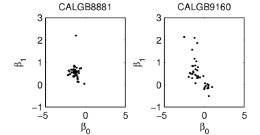
Figure 1: Scatter-plots of the subject-specific regression parameters $\beta_{0}$ and $\beta_{1}$ for the groups in CALGB 8881 and CALGB 9160.

The graphs suggest differences between the joint distribution of $\beta_{0}$ and $\beta_{1}$ which should be included in any analysis which combines these data sets. The results for CALGB9160 also suggest that a nonparametric model is needed to fully describe the shape of the density. A natural Bayesian approach would assume different distributions for each study but construct a dependent prior for these distributions.

In general, suppose that $x\in\mathcal{X}$ denotes the value of covariates then, in a Bayesian nonparametric analysis, a prior needs to be defined across a collection of correlated distributions $\{\tilde{p}_{x}|x\in\mathcal{X}\}$. This problem was initially studied in a seminal paper on dependent Dirichlet processes [34] where generalisations of the Dirichlet process were proposed. Subsequent work used stick-breaking constructions of random measures as a basis for defining such a prior. This work is reviewed by [9]. These priors can usually be represented as

$$\tilde{p}_{x}=\sum_{i=1}^{\infty}w_{i}(x)\delta_{\theta_{i}(x)}$$ (1.1)

where $w_{1}(x),w_{2}(x),\dots$ follow a stick-breaking process for all $x\in\mathcal{X}$. A drawback with this approach is the stochastic ordering of the $w_{i}(x)$’s for any $x\in\mathcal{A}$ which can lead to strange effects in the prior as $x$ varies.

If $\mathcal{A}$ is countable, several other approaches to defining a prior on a collection of random probability measures have been proposed. The Hierarchical Dirichlet process (HDP) [47] assumes that $\tilde{p}_{x}$ are a priori conditionally independent and identically distributed according to a Dirichlet process whose centring measure is itself given a Dirichlet process prior. This construction induces correlation between the elements of $\{\tilde{p}_{x}|x\in\mathcal{A}\}$ in the same way as in parametric hierarchical models. This construction can be extended to more general hierarchical frameworks [see e.g. 46, for a review]. Alternatively, a prior can be defined using the idea of normalized random measures with independent increments which are defined by normalising a completely random measure. The prior is defined on a collection of correlated completely random measures $\{\tilde{\mu}_{x}|x\in\mathcal{A}\}$ which are then normalized for each of $x$, i.e. $\tilde{p}_{x}=\tilde{\mu}_{x}/\tilde{\mu}_{x}(\mathbb{X})$ where $\mathbb{X}$ is the support of $\tilde{\mu}_{x}$. Several specific constructions have been proposed including various forms of superposition [18, 31, 32, 33, 4, 2], the kernel-weighted completely random measures [15, 17] and Lévy copula-based approaches [28, 29, 49]. In this paper, we develop an alternative method for constructing correlated completely random measures which is tractable, whose properties can be derived and for which sampling methods for posterior inference without truncation can be developed. The construction also provides a unifying framework for previously proposed constructions. Indeed, the $\sigma$-stable and gamma vector of dependent random measures, studied in the recent works of [28], [29] and [49] are special cases. Although these papers derive useful theoretical results, their application has been limited by the lack of a sampling methods for posterior inference. The algorithms proposed in this paper can also be used for posterior sampling for these nonparametric priors which is another contribution of the paper.

The paper is organized as follows. Section 2 introduces the concepts of completely random measures, normalized random measures and their multivariate extensions. Section 3 discusses the construction and some properties of a new class of multivariate Lévy process, Compound Random Measures, defined by a score distribution and a directing Lévy process. Section 4 provides a detailed description of Compound Random Measures with a gamma score distribution. Section 5 considers the use of normalized version of Compound Random Measures in nonparametric mixture models including the description of a Markov chain Monte Carlo scheme for inference. Section 6 provides an illustration of the use of these methods in an example and Section 7 concludes.

2 Preliminaries

Let $(\Omega,\mathcal{F},\mathbb{P})$ be a probability space and $(\mathbb{X},\mathcal{X})$ a measure space, with $\mathbb{X}$ Polish and $\mathcal{X}$ the Borel $\sigma$–algebra of subsets of $\mathbb{X}$. Denote by $\mathbb{M}_{\mathbb{X}}$ the space of boundedly finite measures on $(\mathbb{X},\mathcal{X})$, i.e. this means that for any $\mu$ in $\mathbb{M}_{\mathbb{X}}$ and any bounded set $A$ in $\mathcal{X}$ one has $\mu(A)<\infty$. Moreover, $\cal{M}_{\mathbb{X}}$ stands for the corresponding Borel $\sigma$–algebra, see [7] for technical details. The concept of a completely random measure was introduced by [25].

Definition 1.

Let $\tilde{\mu}$ be a measurable mapping from $(\Omega,\mathcal{F},\mathbb{P})$ into ($\mathbb{M}_{\mathbb{X}}$,$\cal{M}_{\mathbb{X}}$) and such that for any $A_{1},\dots,A_{n}$ in $\mathcal{X}$, with $A_{i}\cap A_{j}=\emptyset$ for any $i\neq j$, the random variables $\tilde{\mu}(A_{1}),\dots,\tilde{\mu}(A_{n})$ are mutually independent. Then $\tilde{\mu}$ is called a completely random measure (CRM).

A CRM can always be represented as a sum of two components:

$$\tilde{\mu}=\tilde{\mu}_{c}+\sum_{i=1}^{M}V_{i}\delta_{x_{i}}$$

where the fixed jump points $x_{1},\dots,x_{M}$ are in $\mathbb{X}$ and the non-negative random jumps $V_{1},\dots,V_{M}$ are both mutually independent and independent from $\tilde{\mu}_{c}$. The latter is a completely random measure such that

$$\tilde{\mu}_{c}=\sum_{i=1}^{\infty}J_{i}\delta_{X_{i}}$$

where both the positive jump heights $J_{i}$’s and the $\mathbb{X}$-valued jump locations $X_{i}$’s are random. The measure $\tilde{\mu}_{c}$ is characterized by the Lévy-Khintchine representation which states that

$$\mathbb{E}\left[e^{-\int_{X}f(x)\tilde{\mu}_{c}(dx)}\right]=e^{-\int_{0}^{\infty}\int_{X}[1-e^{-sf(x)}]\bar{\nu}(ds,dx)}$$

where $f:\mathbb{X}\rightarrow\mathbb{R}^{+}$ is a measurable function such that $\int f\tilde{\mu}_{c}<\infty$ almost surely and $\bar{\nu}$ is a measure on $\mathbb{R}^{+}\times\mathbb{X}$ such that

$$\int_{\mathbb{R}^{+}}\int_{B}\min\{1,s\}\bar{\nu}(ds,dx)<\infty$$

for any $B$ in $\mathcal{X}$. The measure $\bar{\nu}$ is usually called the Lévy intensity of $\tilde{\mu}_{c}$. Throughout the paper, we will consider completely random measures without the fixed jump component (i.e. $M=0$). For our purposes, we will focus on the homogeneous case, i.e. Lévy intensities where the height and location contributions are separated. Formally,

$$\bar{\nu}(ds,dx)=\rho(ds)\alpha(dx)$$

where $\rho$ is a measure on $\mathbb{R}^{+}$ and $\alpha$ is a non-atomic measure on $\mathbb{X}$, which is usually called the centring measure. Some famous examples are the Gamma process,

$$\bar{\nu}(ds,dx)=s^{-1}e^{-s}ds\,\alpha(dx),$$

the $\sigma$-stable process,

$$\bar{\nu}(ds,dx)=\frac{\sigma}{\Gamma(1-\sigma)}s^{-1-\sigma}ds\,\alpha(dx),\quad 0<\sigma<1,$$

and the homogeneous Beta process,

$$\bar{\nu}(ds,dx)=\theta s^{-1}(1-s)^{\theta-1}ds\,\alpha(dx),\quad 0<s<1,\quad\theta>0.$$

A general class of processes that includes the gamma and $\sigma$-stable process is the Generalized Gamma process,

$$\bar{\nu}(ds,dx)=\frac{\sigma}{\Gamma(1-\sigma)}s^{-1-\sigma}e^{-as}ds\,\alpha(dx),\quad 0<\sigma<1,\quad a>0$$

Random measures are the basis for building Bayesian nonparametric priors.

Definition 2.

Let $\tilde{\mu}$ be a measure in ($\mathbb{M}_{\mathbb{X}}$,$\cal{M}_{\mathbb{X}}$). A Normalized Random Measure (NRM) is defined as $\tilde{p}=\frac{\tilde{\mu}}{\tilde{\mu}(\mathbb{X})}$.

The definition of a normalized random measure is very general and does not require that the underlying measure is completely random. The Pitman-Yor process (see [39]) is a well-known example of a Bayesian nonparametric priors which cannot be derived by normalizing a completely random measure. In this particular case, the unnormalized measure is obtained through a change of measure of a $\sigma$-stable process. However, many common Bayesian nonparametric priors can be defined as a normalization of a CRM and many other processes can be derived by normalising processes derived from CRMs, see [43]. For instance, it can be shown that the Dirichlet Process, introduced by [14], is a normalized gamma process. Throughout the paper, we will assume that the underlying measure is a CRM and use the acronym NMRI (Normalized Random Measures with independent increments) to emphasize the independence of a CRM on disjoint intervals.

Although nonparametric priors based on normalization are extremely flexible, in many real applications data arise under different conditions and hence assuming a single prior can be too restrictive. For example, using covariates, data may be divided into different units. In this case, one would like to consider different distributions for different units instead of a single common distribution for all the units. In these situations, it is more reasonable to consider vectors of dependent random probability measures.

2.1 Vectors of normalized random measures

Suppose $\tilde{\mu}_{1},\dots,\tilde{\mu}_{d}$ are homogeneous CRMs on $(\mathbb{X},\mathcal{X})$ with respective marginal Lévy intensities

$$\bar{\nu}_{j}(ds,dx)=\nu_{j}(ds)\,\alpha(dx),\qquad\quad j=1,\dots,d.$$ (2.1)

where $\nu_{j}$ is a measure on $\mathbb{R}^{+}$ and $\alpha$ is a non-atomic measure on $\mathbb{X}$. Furthermore, $\tilde{\mu}_{1},\dots,\tilde{\mu}_{d}$ are dependent and the random vector $(\tilde{\mu}_{1},\dots,\tilde{\mu}_{d})$ has independent increments, in the sense that for any $A_{1},\dots,A_{n}$ in $\mathcal{X}$, with $A_{i}\cap A_{j}=\emptyset$ for any $i\neq j$, the random vectors $(\tilde{\mu}_{1}(A_{i}),\dots,\tilde{\mu}_{d}(A_{i}))$ and $(\tilde{\mu}_{1}(A_{j}),\dots,\tilde{\mu}_{d}(A_{j}))$ are independent. This implies that for any set of measurable functions $\bm{f}=(f_{1},\dots,f_{d})$ such that $f_{j}:\mathbb{X}\to\mathbb{R}^{+}$, $j=1,\dots,d$ and $\int|f_{j}|\,d\tilde{\mu}_{j}<\infty$, one has a multivariate analogue of the Lévy-Khintchine representation (see [44], [7] and [10])

$$\mathbb{E}\left[e^{-\tilde{\mu}_{1}(f_{1})-\cdots-\tilde{\mu}_{d}(f_{d})}\right]=\exp\left\{-\psi^{*}_{\rho,d}(\bm{f})\right\}$$ (2.2)

where $\tilde{\mu}_{j}(f_{j})=\int f_{j}\,d\tilde{\mu}_{j}$,

$$\psi^{*}_{\rho,d}(\bm{f})=\int_{\mathbb{X}}\int_{(0,\infty)^{d}}\left[1-\mathrm{e}^{-s_{{}_{1}}f_{1}(x)-\cdots-s_{d}f_{d}(x)}\right]\;\rho_{d}(ds_{1},\dots,ds_{d})\>\alpha(dx)$$ (2.3)

and

$$\int_{(0,\infty)^{d-1}}\rho_{d}(ds_{1},\dots,ds_{j-1},A,ds_{j+1},\dots,ds_{d})=\int_{A}\nu_{j}(ds).$$ (2.4)

The representation (2.1) implies that the jump heights of $(\tilde{\mu}_{1},\dots,\tilde{\mu}_{d})$ are independent from the jump locations. Moreover, these jump locations are common to all the CRMs and are governed by $\alpha$. It is worth noting that, since $(\tilde{\mu}_{1},\ldots,\tilde{\mu}_{d})$ has independent increments, its distribution is characterized by a choice of $f_{1},\ldots,f_{d}$ in (2.2) such that $f_{j}=\lambda_{j}\,1_{A}$ for any set $A$ in $\mathcal{X}$, $\lambda_{j}\in\mathbb{R}^{+}$ and $j=1,\ldots,d$. In this case

$$\psi^{*}_{\rho,d}(\bm{f})=\alpha(A)\,\psi_{\rho,d}(\bm{\lambda})$$

where $\bm{\lambda}=(\lambda_{1},\ldots,\lambda_{d})$ and

$$\psi_{\rho,d}(\bm{\lambda})=\int_{(\mathbb{R}^{+})^{d}}\left[1-\mathrm{e}^{-\langle\bm{\lambda},\bm{s}\rangle}\right]\rho_{d}(ds_{1},\dots,ds_{d})$$ (2.5)

where $\bm{s}=(s_{1},\ldots,s_{d})$ and $\langle\bm{\lambda},\bm{s}\rangle=\sum_{j=1}^{d}\lambda_{j}s_{j}$.

We close the section with the definition of vectors of normalized random measures with independent increments.

Definition 3.

Let ($\tilde{\mu}_{1},\dots,\tilde{\mu}_{d}$) be a vector of CRMs on $\mathbb{X}$ and let $\tilde{p}_{j}=\frac{\mu_{j}}{\mu_{j}(\mathbb{X})}$, $j=1,\dots,d$. The vector

$$\tilde{p}=(\tilde{p}_{1},\dots,\tilde{p}_{d})$$ (2.6)

is called a vector of dependent normalized random measures with independent increments on $(\mathbb{X},\mathcal{X})$.

3 Compound Random Measures

In this section, we will define a general class of vectors of NRMI that incorporates many recently proposed priors built using normalization, see for instance [28], [29], [49], [18] and [32]. Before introducing the formal definition of Compound Random Measures, we want to provide an intuitive illustration of the model. Consider the following dependent random probability measures:

$$\tilde{p}_{1}=\sum_{i\geq 1}\pi_{1,i}\delta_{X_{i}},\,\dots,\,\tilde{p}_{d}=\sum_{i\geq 1}\pi_{d,i}\delta_{X_{i}},$$

where

$$\pi_{j,i}=\frac{m_{j,i}J_{i}}{\sum_{l}m_{j,l}J_{l}}.$$ (3.1)

The $m_{j,i}$’s are perturbation coefficients that identify specific features of the $j$-th random measure and they are independent and identically distributed across the random measures. The shared jumps $(J_{i})_{i\geq 1}$ lead to dependence among the $\tilde{p}_{j}$. In the next section, we will provide a formal definition of Compound random measures in terms of its multivariate Lévy intensity.

3.1 Definition

Let $(\tilde{\mu}_{1},\dots,\tilde{\mu}_{d})$ be a vector of homogeneous CRMs on $\mathbb{X}$, i.e. the Lévy intensity $\nu_{j}$ of the measure $\tilde{\mu}_{j}$ is

$$\bar{\nu}_{j}(ds,dx)=\nu_{j}(ds)\,\alpha(dx),\quad j=1,\dots,d.$$

Following the notation in Eq. (2.3), we want to define a $\rho_{d}$ such

$$\int_{(0,\infty)^{d-1}}\rho_{d}(ds_{1},\dots,ds_{j-1},A,ds_{j+1},\dots,ds_{d})=\int_{A}\nu_{j}(ds)$$ (3.2)

for any $j=1,\dots,d$. In this setting we can define a compound random measure.

Definition 4.

A Compound random measure (CoRM) is a vector of CRMs defined by a score distribution $h$ and a directing Lévy process with intensity $\nu^{*}$ such that

$$\rho_{d}(ds_{1},\dots,ds_{d})=\int h(s_{1},\dots,s_{d}|z)\,ds_{1}\cdots ds_{d}\,\nu^{\star}(dz)$$ (3.3)

where $h(\cdot|z)$ is the probability mass function or probability density function of the score distribution with parameters $z$ and $\nu^{\star}$ is the Lévy intensity of the directing Lévy process which satisfies the condition

$$\int\int\min(1,\parallel\bm{s}\parallel)h(s_{1},\dots,s_{d}|z)\,d\bm{s}\,\nu^{\star}(dz)<\infty$$

where $\parallel\bm{s}\parallel$ is the Euclidean norm of the vector $\bm{s}=(s_{1},\dots,s_{d})$.

The compound Poisson process with jump density $h$ is a compound random measure with a score density $h$ and whose directing Lévy process is a Poisson process. Therefore, compound random measures can be seen as a generalisation of compound Poisson processes. It is straightforward to show that $\tilde{\mu}_{1},\dots,\tilde{\mu}_{d}$ can be expressed as

$$\tilde{\mu}_{j}=\sum_{i=1}^{\infty}m_{j,i}J_{i}\delta_{X_{i}}$$ (3.4)

where $m_{1,i},\dots,m_{d,i}\stackrel{{\scriptstyle i.i.d.}}{{\sim}}h$ are scores and

$$\tilde{\eta}=\sum_{i=1}^{\infty}J_{i}\delta_{X_{i}}$$

is a CRM with Lévy intensity $\nu^{\star}(ds)\alpha(dx)$. This makes the structure of the prior much more explicit. The random measures share the same jump locations (which have distribution $\alpha/\alpha(\mathbb{X})$) but the $i$-th jump has a height $m_{j,i}J_{i}$ in the $j$-th measure and so the jump heights are re-scaled by the score (a larger score implies a larger jump height). Clearly, the shared factor $J_{i}$ leads to dependence between the jump heights in each measure.

The construction can be seen in an alternative way, in terms of (augmented) dependent Poisson random measures. Indeed,

$$\mathbb{E}\left[e^{-\lambda\tilde{\mu}_{j}(A)}\right]=e^{-\alpha(A)\int_{0}^{\infty}(1-e^{-\lambda s})\int h_{j}(s|z)\nu^{*}(dz)ds}.$$

If in the exponent we set $s=mz$, then

$$\mathbb{E}\left[e^{-\lambda\tilde{\mu}_{j}(A)}\right]=e^{-\alpha(A)\int_{0}^{\infty}(1-e^{-\lambda mz})\int zh_{j}(mz|z)\nu^{*}(dz)dm}$$

which entails that $\tilde{\mu}_{j}(dx)=\int_{0}^{\infty}\int mzN_{j}(dm,dz,dx)$ where

$$N_{j}=\sum_{i\geq 1}\delta_{(m_{j,i},J_{i},X_{i})}$$

is a Poisson random measure with intensity on $(0,+\infty)^{2}\times\mathbb{X}$ and with Lévy intensity given by $\alpha(dx)zh_{j}(mz|z)\nu^{*}(dz)$. This is identical to the distribution given by (3.4). The Poisson processes $(N_{1},\dots,N_{d})$ are dependent because they share $\{(J_{i},X_{i}):i\geq 1\}$. The term “augmentation” here refers to the fact that the Poisson random measures that characterize the CRMs are typically on $(0,+\infty)\times\mathbb{X}$. A third dimension is introduced to account the heterogeneity across different measures.

To ensure the existence of the vectors of normalized CoRM, as introduced in Definition 3, the following condition must be satisfied for each $j=1,\dots,d$:

$$\nu_{j}((0,+\infty))=\int_{0}^{+\infty}\int h_{j}(s|z)\nu^{\star}(dz)ds=+\infty$$

where $h_{j}(s|z)=\int h(s_{1},\dots,s_{j-1},s,ds_{j+1},\dots,s_{d}|z)ds_{1}\cdots ds_{j-1}ds_{j+1}\cdots ds_{d}$. If this condition does not hold true, then $\tilde{\mu}_{j}(\mathbb{X})=0$ with positive probability and the normalization does not make sense, see [43].

In this paper, we will concentrate on the sub-class of CoRMs with a continuous score distribution which has independent dimensions and a single scale parameter so that

$$h(s_{1},\dots,s_{d}|z)=z^{-d}\prod_{j=1}^{d}f(s_{j}/z)\,$$

where $f$ is a univariate distribution. This implies that each marginal process has the same Lévy intensity of the form

$$\nu_{j}(ds)=\nu(ds)=\int z^{-1}f(s|z)\,ds\,\nu^{\star}(dz).$$ (3.5)

In Section 5.2, algorithms are introduced to sample from the posterior of a hierarchical mixture models whose parameters are driven by a vector of normalized compound random measures. These samplers depend crucially on knowing the form of the Laplace Exponent and its derivatives. Some general results about the Laplace exponent and the dependence are available if we assume that the density $z^{-1}f(s_{i}/z)$ admits a moment generating function.

Theorem 3.1.

Let

$$M_{z}^{f}(t)=\int e^{ts}z^{-1}f(s/z)ds$$

be the moment generating function of $z^{-1}f(s_{j}/z)$ and suppose that it exists. Then

$$\psi_{\rho,d}(\lambda_{1},\dots,\lambda_{d})=\int\left(1-\prod_{j=1}^{d}M_{z}^{f}(-\lambda_{j})\right)\nu^{\star}(z)dz.$$ (3.6)

The proof of the Theorem stated above is in the appendix as well as a further result about the derivatives of the Laplace exponent.

4 CoRMs with independent gamma distributed scores

In this paper, we will focus on exponential or gamma score distributions. Throughout the paper we will write $\mbox{Ga}(\phi)$ to be a gamma distribution (or density) with shape $\phi$ and mean $\phi$ which has density

$$f(x)=\frac{1}{\Gamma(\phi)}x^{\phi-1}\exp\{-x\}.$$ (4.1)

This implies that $z^{-1}f(y/z)$ is the density of a gamma distribution with shape parameter equal to $\phi$ and mean $\phi\,z$. The Lévy intensities $\nu$ and $\nu^{\star}$ and the score density $f$ are linked by (3.5) and a CoRM can be defined by either deriving $\nu^{\star}$ for a fixed choice of $f$ and $\nu$ or by directly specifying $f$ and $\nu^{\star}$. In this latter case, it is interesting to consider the properties of the induced $\nu$.

Standard inversion methods can be used to derive the form of $\nu^{*}$. Equation (3.5) implies that

$$\nu(s)=\int z^{-1}\frac{1}{\Gamma(\phi)}\left(\frac{s}{z}\right)^{\phi-1}\exp\left(-\frac{s}{z}\right)\nu^{*}(z)dz$$

The change of variable $t=z^{-1}$ leads to

$$\nu(s)=\frac{s^{\phi-1}}{\Gamma(\phi)}\int\exp\left(-st\right)t^{\phi-2}\nu^{*}\left(\frac{1}{t}\right)dt.$$

The above integral can be seen as the classical Laplace transform of the function $f(t)=t^{\phi-2}\nu^{*}\left(\frac{1}{t}\right)$. If we denote by $\mathcal{L}$ the Laplace transform then

$$\nu(s)=\frac{s^{\phi-1}}{\Gamma(\phi)}\mathcal{L}(f(t))(s)$$

This means that

$$\nu^{*}\left(\frac{1}{t}\right)=t^{2-\phi}\mathcal{L}^{-1}\left(\frac{\Gamma(\phi)}{s^{\phi-1}}\nu(s)\right)(t)$$

where $\mathcal{L}^{-1}$ is the inverse Laplace transform. This ensures the unicity of $\nu^{*}$. The forms for some particular choices of marginal process are shown in Table 1.

$\nu^{*}(z)$	Support	Marginal Process
$z^{-1}(1-z)^{\phi-1}$	$0<z<1$	Gamma
$z^{-\sigma-1}\frac{\Gamma(\phi)}{\Gamma(\phi+\sigma)\Gamma(1-\sigma)}$	$z>0$	$\sigma$-stable
$\frac{\sigma\Gamma(\phi)}{\Gamma(\phi+\sigma)\Gamma(1-\sigma)}z^{-\sigma-1}(1-a\,z)^{\sigma+\phi-1}$	$0<z<1/a$	Gen. Gamma

Table 1: The form of directing Lévy intensity in a CoRM which leads to particular marginal processes.

The results are surprising. A gamma marginal process arises when the directing Lévy process is a Beta process and a $\sigma$-stable marginal process arises when the directing Lévy process is also a $\sigma$-stable process. Generalized gamma marginal processes lead to a directing Lévy process which is a generalization of the Beta process (with a power of $z$ which is less than 1) and re-scaled to the interval $(0,1/a)$. In fact, if we use a gamma score distribution with shape $\phi$ and mean $a\phi$ which has density

$$f(x)=\frac{1}{a^{\phi}\Gamma(\phi)}x^{\phi-1}\exp\{-x/a\},$$ (4.2)

the directing Lévy intensity is a stable Beta [45] of the form

$$\nu^{\star}(z)=\frac{a^{\sigma+1}\sigma}{\phi}\frac{\Gamma(\phi+1)}{\Gamma(\phi+\sigma)\Gamma(1-\sigma)}z^{-\sigma-1}(1-z)^{\sigma+\phi-1},\qquad 0<z<1.$$

Remark.

Several authors have previously considered hierarchical models where $\tilde{\mu}_{1},\dots,\tilde{\mu}_{d}$ followed i.i.d. CRM (or NRMI) processes whose centring measure are given a CRM (or NRMI) prior. This construction induces correlation between $\tilde{\mu}_{1},\dots,\tilde{\mu}_{d}$ and the hierarchical Dirichlet process is a popular example but we will concentrate on a hierarchical Gamma process [see e.g. 37]. In this case, $\tilde{\mu}_{1},\dots,\tilde{\mu}_{d}$ follow independent Gamma processes with centring measure $\alpha$ which also follows a Gamma process. This implies that we can write

$$\alpha=\sum_{i=1}^{\infty}s_{i}\delta_{\theta_{i}}$$

and we can write

$$\tilde{\mu}_{j}=\sum_{i=1}^{\infty}J_{j,i}\delta_{\theta_{i}}$$ (4.3)

where $J_{j,i}\sim\mbox{Ga}(s_{i})$. This can be represented as a CoRM process where $\alpha$ is the directing Lévy process and the score distribution is $\prod_{j=1}^{d}\mbox{Ga}(s_{i})$ where $s_{i}$ controls the shape of the conditional distribution of $J_{j,i}$. This contrasts with the processes considered in this section with independent gamma scores which multiply the jumps in the directing Lévy process and lead to a marginal gamma process for $\tilde{\mu}_{j}$ (unlike the hierarchical model). These processes can be written in the form of (4.3) with $J_{j,i}$ having a gamma distribution with shape $\phi$ and mean $\phi s_{i}$, and $\alpha$ chosen to follow a beta process.

Remark.

This paper is focused on Gamma scores but the class of CoRMs is very wide and other choices can be considered. For instance, if $Beta(\alpha,1)$ scores are selected, i.e.

$$f(x)=\alpha x^{\alpha-1}\qquad\alpha>0,\quad 0<x<1$$

then it is possible to introduce a multivariate version of the Beta process. Let $\nu(s)=\theta s^{-1}(1-s)^{\theta-1}$, $0<s<1$, i.e. the Lévy intensity of the jumps of a Beta process, then $\nu^{\star}(z)$ is the solution of the integral equation

$$\nu(s)=\int_{s}^{1}f(s/z)s^{-1}\nu^{\star}(z)\,dz,\quad 0<s<1$$

A simple application of the fundamental Theorem of Calculus leads to

$$\nu^{\star}(z)=\theta z^{-1}(1-z)^{\theta-1}+\frac{\theta(\theta-1)}{\alpha}(1-z)^{\theta-2}$$

which is the sum of $\nu(\cdot)$, the Lévy intensity of the original Beta process, and a compound Poisson process (if $\theta>1$) with intensity $\theta/\alpha$ and jump distribution $Beta(1,\theta-1)$. This is well-defined if $\theta>1$.

It is interesting to derive the resulting multivariate Lévy intensities which can be compared with similar results in [28], [29] and [49].

Theorem 4.1.

Consider a CoRM process with independent $\mbox{Ga}(\phi,1)$ distributed scores. If the CoRM process has gamma process marginals then

$$\rho_{d}(s_{1},\dots,s_{d})=\frac{(\prod_{j=1}^{d}s_{j})^{\phi-1}}{[\Gamma(\phi)]^{d-1}}|\bm{s}|^{-\frac{d\phi+1}{2}}e^{-\frac{|\bm{s}|}{2}}W_{\frac{(d-2)\phi+1}{2},-\frac{d\phi}{2}}(|\bm{s}|)$$ (4.4)

where $|\bm{s}|=s_{1}+\dots+s_{d}$ and $W$ is the Whittaker function. If the CoRM process has $\sigma$-stable process marginals then

$$\rho_{d}(s_{1},\dots,s_{d})=\frac{(\prod_{j=1}^{d}s_{j})^{\phi-1}}{[\Gamma(\phi)]^{d-1}}\frac{\Gamma(\sigma+d\phi)}{\Gamma(\sigma)\Gamma(1-\sigma)}|\bm{s}|^{-\sigma-d\phi}.$$ (4.5)

The result is proved in the appendix with the following corollary.

Corollary 4.1.

Consider a CoRM process with independent exponentially distributed scores. If the CoRM has gamma process marginals we recover the multivariate Lévy intensity of [29],

$$\rho_{d}(s_{1},\dots,s_{d})=\sum_{j=0}^{d-1}\frac{(d-1)!}{(d-1-j)!}|\bm{s}|^{-j-1}e^{-|\bm{s}|}.$$

Otherwise, if $\sigma$-stable marginals are considered then we recover the multivariate vector introduced in [28] and [49],

$$\rho_{d}(s_{1},\dots,s_{d})=\frac{(\sigma)_{d}}{\Gamma(1-\sigma)}|\bm{s}|^{-\sigma-d}.$$

Alternatively, we can specify $\nu^{\star}$ and derive $\nu$. The forms for some particular processes are shown in Table 2

$\nu(s)$	Directing Lévy process
$\frac{\Gamma(\theta+1)}{\Gamma(\phi)}s^{-1}\exp\{-s\}U(\theta-\phi,1-\phi,s)$	Beta
$2\frac{1}{\Gamma(\phi)}\frac{\sigma}{\Gamma(1-\sigma)}s^{(\phi-\sigma)/2-1}a^{(\sigma+\phi)/2}K_{\sigma+\phi}\left(2\sqrt{as}\right)$	Gen. Gamma

Table 2: The Lévy intensity of the marginal process in a CoRM with different directing Lévy processes.

where $U$ is the confluent hypergeometric function of the second kind and $K$ is the modified Bessel function of the second kind.

Remark.

There are several special cases if $\nu^{\star}$ is the Lévy intensity of a Beta process. Firstly, $U(\theta-\phi,1-\phi,s)=1$ if $\theta=\phi$ and $\nu$ is the Lévy intensity of a gamma process. If $\phi=2\theta-1$,

$$U(\theta-\phi,1-\phi,s)=\pi^{-1/2}\exp\{s/2\}s^{1/2-\theta+\phi}K_{\theta-1/2}(s/2).$$

When $\theta=1$, $U(1-\phi,1-\phi,s)=\exp\{s\}\int_{s}^{\infty}u^{-(1-\phi)}\exp\{-u\}\,du$. The limits as $s\rightarrow 0$ are

$$U(\theta-\phi,1-\phi,s)\rightarrow\left\{\begin{array}[]{lc}\Gamma(\phi)/\Gamma(\theta)+O(|s|^{\phi})&0<\phi<1\\ 1/\Gamma(1+\theta-\phi)+O(|s\log s|)&\phi=1\\ \Gamma(\phi)/\Gamma(\theta)+O(|s|)&\phi>1\end{array}\right.$$

Therefore, these processes have a Lévy intensity similar to the Lévy intensity of the gamma process close to zero for any choice of $\phi$ and $\theta$. The tails of the Lévy intensity are exponential. Therefore, the process has similar properties to the gamma process.

Remark.

The generalized gamma process contains some special cases and the Lévy intensity of the marginal process for these process are shown in Table 3.

$\nu(s)$	Directing Lévy process
$2\frac{1}{\Gamma(\phi)}s^{\phi/2-1}K_{\phi}\left(2\sqrt{s}\right)$	Gamma Process
$\frac{\Gamma(\phi+\sigma)}{\Gamma(\phi)}\frac{\sigma}{\Gamma(1-\sigma)}s^{-1-\sigma}$	$\sigma$-stable Process.

Table 3: The Lévy intensity of the marginal process in a CoRM with different directing Lévy processes.

With a generalized gamma directing Lévy process, It is straightforward to show that

$$\nu(s)\approx\sigma\frac{\Gamma(\sigma+\phi)}{\Gamma(\phi)\Gamma(1-\sigma)}s^{-\sigma-1}$$

for small $s$. Therefore, the Lévy intensity close to zero is similar to the Lévy intensity of $\sigma$-stable process with parameter $\sigma$. For large $s$, we have

$$\nu(s)s\propto\sqrt{\pi}\frac{1}{\Gamma(\phi)}\frac{\sigma}{\Gamma(1-\sigma)}(as)^{(\phi+\sigma)/2-1/4}s^{-1-\sigma}\exp\{-2\sqrt{a}s^{1/2}\}.$$

Therefore, the tails will decays like $\exp\{-s^{1/2}\}$.

The next Theorems will provide an expression of the Laplace exponent when the scores are gamma distributed with $\phi\geq 1$ such that $\phi\in\mathbb{N}$. We want to stress the importance of the the Laplace transform in the Bayesian nonparametric setting. Indeed, it is the basis to prove theoretical results of the prior of interest. For instance, [28], [29] and [49] used the Laplace Transform to derive some distributional properties such as correlation, partition structure and mixed moments. Additionally, we will see that the Laplace transform plays a role in the novel sampler proposed in this paper.

Theorem 4.2.

Consider a CoRM process with independent $\mbox{Ga}(\phi,1)$ distributed scores. Suppose $\phi\geq 1$ such that $\phi\in\mathbb{N}$. Let $\bm{\lambda}\in(\mathbb{R}^{+})^{d}$ be a vector such that it consists of $l\leq d$ distinct values denoted as $\bm{\tilde{\lambda}}=(\tilde{\lambda}_{1},\ldots,\tilde{\lambda}_{l})$ with respective multiplicities $\bm{n}=(n_{1},\dots,n_{l})$. Then

$$\psi_{\rho,d}(\bm{\lambda})=\psi_{\rho,d}(\bm{\tilde{\lambda}},\bm{n})=\frac{[\Gamma(\phi)]^{l}}{\prod_{i=1}^{l}[\tilde{\lambda}_{i}^{\phi-1}\Gamma(n_{i}\phi)]}\left(\prod_{i=1}^{l}\frac{\partial^{(n_{i}-1)\phi}}{\partial^{(n_{i}-1)\phi}\tilde{\lambda}_{i}}\right)\left(\Upsilon_{l}^{\phi}(\bm{\tilde{\lambda}})\prod_{i=1}^{l}\tilde{\lambda}_{i}^{n_{i}\phi-1}\right),$$

where

$$\Upsilon^{\phi}_{l}(\bm{\tilde{\lambda}})=\int\left(1-\prod_{i=1}^{l}\frac{1}{(1+z\tilde{\lambda}_{i})^{\phi}}\right)\nu^{\star}(z)dz.$$

The proof of the previous Theorem is based on the result provided in Theorem 3.6 since the moment generating of a Gamma distribution exists and it is explicit.

To compute the expression of $\Upsilon_{l}^{\phi}(\bm{\tilde{\lambda}})$ we need to define the following set

$$A_{\phi,j}=\{\bm{k}\in\{1,\ldots,\phi\}^{j}:\>|\bm{k}|=\phi\}\qquad\phi\geq j.$$

Theorem 4.3.

Consider a CoRM process with independent $\mbox{Ga}(\phi,1)$ distributed scores. Suppose $\phi\geq 1$ such that $\phi\in\mathbb{N}$. Let $\Lambda(\bm{\tilde{\lambda}},\bm{z})=(1-\sum_{h=1}^{j-1}z_{h})\tilde{\lambda}_{i_{j}}+\sum_{h=1}^{j-1}\tilde{\lambda}_{i_{h}}z_{h}$ be a function defined on the (j-1)-dimensional simplex

$$\Delta_{j-1}=\{\mathbf{z}\in(0,1)^{j-1}:z_{1}+\cdots+z_{j-1}<1\}$$

with the convention that $\Delta_{0}=[0,1]$ . Let

$$a_{i}(\bm{\tilde{\lambda}})=\frac{\tilde{\lambda}_{i}^{l-1}}{\prod_{\begin{subarray}{c}j=1\\ j\neq i\end{subarray}}^{l}(\tilde{\lambda}_{i}-\tilde{\lambda}_{j})}\qquad i=1,\dots,l.$$

then

$$\Upsilon_{l}^{\phi}(\bm{\tilde{\lambda}})=\left\{\begin{array}[]{ll}\phi!\displaystyle\sum_{j=1}^{\phi}\sum_{\bm{k}\in A_{\phi,j}}\sum_{0<i_{1}<i_{2}<\cdots<i_{j}\leq l}\frac{a_{i_{1}}^{k_{1}}(\bm{\tilde{\lambda}})\cdots a_{i_{j}}^{k_{j}}(\bm{\tilde{\lambda}})}{k_{1}!\dots k_{j}!}C(i_{1},\dots,i_{j};\bm{k};\bm{\tilde{\lambda}})&\mbox{ if }l>1\\ \psi(\lambda_{1})&\mbox{ if }l=1\end{array}\right.$$

where

$$C(i_{1},\dots,i_{j};\bm{k};\bm{\tilde{\lambda}})=\Gamma(\phi)\int_{\Delta_{j-1}}\left((1-\sum_{h=1}^{j-1}z_{h})^{k_{j}}\prod_{h=1}^{j-1}\frac{z_{h}^{k_{h}-1}}{\Gamma(k_{h})}\right)\psi\left(\Lambda(\bm{\tilde{\lambda}},\bm{z})\right)d\bm{z}$$

For the above integral we assume the usual convention that $\sum_{i}^{j}=0$ and $\prod_{i}^{j}=1$ whenever $i>j$.

In the following Corollary, the expression of the Laplace exponent is recovered for the special case of a CoRM with independent exponentially distributed scores.

Corollary 4.2.

Consider a CoRM process with independent exponentially distributed scores. It follows that

$$\psi_{\rho,d}(\bm{\lambda})=\psi_{\rho,d}(\bm{\tilde{\lambda}},\bm{n})=\left(\prod_{i=1}^{l}\frac{1}{\Gamma(n_{i})}\frac{\partial^{(n_{i}-1)}}{\partial^{(n_{i}-1)}\tilde{\lambda}_{i}}\right)\left(\Upsilon_{I}(\bm{\tilde{\lambda}})\prod_{i=1}^{l}\tilde{\lambda}_{i}^{(n_{i}-1)}\right),$$

$$\Upsilon_{l}(\bm{\tilde{\lambda}})=\left\{\begin{array}[]{ll}\sum_{i=1}^{l}a_{i}(\bm{\tilde{\lambda}})\psi(\lambda_{i})&\mbox{ if }l>1\\ \psi(\lambda_{1})&\mbox{ if }l=1\end{array}\right..$$

The proof of the corollary is omitted since it is a direct application of the results of the previous Theorems. Note that, if the vector has Gamma process marginals, i.e. $\psi(\lambda_{i})=\log(1+\lambda_{i})$, then we recover the results in [29]. If the vector has $\sigma$-stable process marginals, i.e. $\psi(\lambda_{i})=\lambda_{i}^{\sigma}$, then we recover the result in [28] and [49].

Finally, we close the section with some results about the dependence structure of CoRM processes. A useful description of the dependence of a vector of CRMs is given by the Lévy copula. A Lévy Copula is a mathematical tool that allows the construction of multivariate Lévy intensities with fixed marginals, see appendix. The following Theorem displays the underlying Lévy Copula of a compound random measure.

Theorem 4.4.

Let $\rho_{d}$ be the compound random measure defined in (3.3) and let $F$ be the the distribution function of $f$. The underlying Lévy Copula of the compound random measure is

$$C(s_{1},\dots,s_{d})=\int\nu^{\star}(z)\prod_{j=1}^{d}(1-F(z^{-1}U^{-1}(s_{j})))dz$$

where $U^{-1}$ is the inverse of the tail integral function $U(x):=\int_{x}^{\infty}\nu(s)\,ds$.

Furthermore, it is possible to prove a result similar to Proposition 5 in [29]. This result gives a close formula for the mixed moments of two dimensions of a CoRM process. The result is expressed in terms of an ordering on sets $\bm{0}\prec\bm{s}_{1}\prec\,\cdots\,\prec\bm{s}_{j}$ which is defined in [5].

Theorem 4.5.

Consider a CoRM process with an independent $\mbox{Ga}(\phi,1)$ distributed scores. Let $\bm{q}=(q_{1},\dots,q_{d})$ and let $p_{j}(\bm{q},k)$ be the set of vectors $(\bm{\eta},\bm{s}_{1},\ldots,\bm{s}_{j})$ such that the coordinates of $\bm{\eta}=(\eta_{1},\ldots,\eta_{j})$ are positive and such that $\sum_{i=1}^{j}\eta_{i}=k$. Moreover, $\bm{s}_{i}=(s_{1,i},\dots,s_{d,i})$ are vectors such that $\bm{0}\prec\bm{s}_{1}\prec\,\cdots\,\prec\bm{s}_{j}$ and $\sum_{i=1}^{j}\eta_{i}(s_{1,i}+\cdots+s_{d,i})=k=q_{1}+\dots+q_{d}$. Then,

$$\begin{split}\mathbb{E}\left[\prod_{i=1}^{d}\{\tilde{\mu}_{i}(A)\}^{q_{i}}\right]&=q_{1}!\cdots q_{d}!\>\sum_{k=1}^{\mid\bm{q}\mid}[\alpha(A)]^{k}\>\times\>\\ &\times\sum_{j=1}^{\mid\bm{q}\mid}\>\sum_{p_{j}(\bm{q},k)}\>\prod_{i=1}^{j}\frac{1}{\eta_{i}!}\left[\left(\prod_{l=1}^{d}\frac{(\phi)_{s_{l,i}}}{s_{l,i}!}\right)\int z^{{s_{1,i}+\cdots+s_{d,i}}}\nu^{\star}(z)dz\right]^{\eta_{i}}\end{split}$$

where $\mid\bm{q}\mid=q_{1}+\cdots+q_{d}$.

Remark.

For instance, suppose that the CoRM process has generalized gamma process marginals. Then,

$$\begin{split}\int z^{s_{1,i}+\cdots+s_{d,i}}\nu^{\star}(z)dz=\frac{\sigma a^{\sigma-(s_{1,i}+\cdots+s_{d,i})}}{\Gamma(1-\sigma)}B(k-\sigma-1,\sigma+\phi).\end{split}$$

5 Normalized Compound Random Measures

Vectors of correlated random probability measures can be defined by normalizing each dimension of a CoRM process. This will be called a Normalized Compound Random Measure (NCoRM) and is defined by a score distribution, a directing Lévy process and a centring measure of the CoRM. The results derived in Table 1 can be used to define a NCoRM with a particular marginal process. For example, an NCoRM with Dirichlet process marginals arises by normalizing each dimension of a CoRM with gamma process marginals.

In specifying an NCoRM prior, it is useful to have a method of choosing the parameters of the score distribution to give a particular level of dependence. We describe two possible methods. It is possible to compute the covariance of a two dimensions of an NCoRM process. Indeed, following [29],

$$\begin{split}\mbox{Cov}\left[\tilde{p}_{1}(A),\,\tilde{p}_{2}(B)\right]&=\left\{\alpha(A\cap B)-\frac{\alpha(A)\alpha(B)}{\alpha(\mathbb{X})}\right\}\\[7.0pt] &\qquad\times\>\int_{(\mathbb{R}^{+})^{2}}g_{\rho}(1,1;\lambda_{1},\lambda_{2})\,\mathrm{e}^{-\alpha(\mathbb{X})\psi_{\rho}(\lambda_{1},\lambda_{2})}\>d\lambda_{1}\,d\lambda_{2}\end{split}$$ (5.1)

where $g_{\rho}$ is the function introduced in Equation (B.1). This result can be used to specify any parameters of the score distribution (or a prior for those parameters). Alternatively, if the scores are independent, the ratio of the same jump heights in the $i$-th and $j$-th dimension has the same distribution as the ratio of two independent random variables following the score distribution. For example, if the scores are independent and follow a gamma distribution with shape $\phi$ is chosen, this ratio follows an $F$-distribution with $\phi$ and $\phi$ degrees of freedom.

5.1 Links to other processes

Corollary 4.1 shows how the priors described in [28], [29] and [49] can be expressed in the CoRM framework. The CNMRI process [18][see also 32, 4] can also be expressed in the NCoRM framework. The CNMRI prior express the random measure $\tilde{\mu}_{g}$ as

$$\tilde{\mu}_{j}=\sum_{k=1}^{q}D_{jk}\tilde{\mu}^{\star}_{k}$$

where $D$ is a $(d\times q)$-dimensional selection matrix (with elements either equal to 0 or 1) and $\tilde{\mu}^{\star}_{1},\dots,\tilde{\mu}^{\star}_{q}$ are independent CRMs where $\tilde{\mu}^{\star}_{k}$ has Lévy intensity $M_{k}\nu^{\star}(ds)\bar{\alpha}(dx)$ for a probability measure $\bar{\alpha}$. A CNRMI process can be represented by a vector of CoRMs with score probability mass function

$$g(s_{1}=D_{1i}z,\dots,s_{d}=D_{di}z|z)=\frac{M_{i}}{\sum_{k=1}^{q}M_{k}},$$

directing Lévy intensity $\nu^{\star}$ and centring measure $\bar{\alpha}\sum_{k=1}^{q}M_{k}$. A CoRM process with independent scores can be used to construct a sub-class of CNRMI processes. A CoRM has a score distribution of the form $f(s)=\pi\delta_{s=1}+(1-\pi)\delta_{s=0}$, directing Lévy intensity $\nu^{\star}(ds)$ and centring measure $M\bar{\alpha}$ is identical to an unnormalized CNRMI process with $q=2^{d}$, a $D$ whose rows are the binary expansion of $\{0,1,\dots,2^{d}-1\}$ and $M_{k}=M\prod_{l=1}^{d}\pi^{D_{kl}}(1-\pi)^{1-D_{kl}}$. A more general class of unnormalized CNRMI processes with $M_{k}=M\prod_{l=1}^{d}\pi_{l}^{D_{kl}}(1-\pi_{l})^{1-D_{kl}}$ which corresponds to a vector of CRMs such that

$$\rho_{d}(ds_{1},\dots,ds_{d})=\int z^{-d}\prod_{j=1}^{d}f_{j}(s_{j}/z)\,ds_{1}\cdots ds_{d}\,\nu^{\star}(dz)$$ (5.2)

where $f_{j}(m)=\pi_{j}\delta_{m=1}+(1-\pi_{j})\delta_{m=0}$.

5.2 Computational Methods

We describe methods for fitting a nonparametric mixture model where the mixing measure is given a NCoRM prior. We assume that the data can be divided into $d$ groups and $y_{j,1},\dots,y_{j,n_{j}}$ are the observations in the $j$-th group. The data are modelled as

$$y_{j,i}\stackrel{{\scriptstyle ind.}}{{\sim}}k(y_{j,i}|\zeta_{j,i}),\quad\zeta_{j,i}\sim\tilde{p}_{j},\quad i=1,2,\dots,n_{j},\quad j=1,\dots,d$$

where $k(y|\theta)$ is a probability density function for $y$ with parameter $\theta$ and $\tilde{p}_{1},\dots,\tilde{p}_{d}$ are given an NCoRM prior. Using the notation of (3.4), we write

$$\tilde{p}_{j}=\frac{\tilde{\mu}_{j}}{\tilde{\mu}_{j}(\mathbb{X})}=\frac{\sum_{k=1}^{\infty}m_{j,k}\,J_{k}\,\delta_{\theta_{k}}}{\sum_{k=1}^{\infty}m_{j,k}\,J_{k}}.$$

Direct simulation from the posterior distribution is impossible since there are an infinite number of parameters. Several MCMC methods have been introduced which circumvent this problem in the class of normalized random measure mixtures. [13] describe an auxiliary variable method which involves integrating out the unnormalized random measure whereas [20] introduce a slice sampling method. We consider extending both methods to NCoRM mixtures.

We use the notation $m=(m_{j,k})$, $J=(J_{1},J_{2},\dots)$ and $\theta=(\theta_{1},\theta_{2},\dots)$. The posterior distribution can be expressed in a suitable form for MCMC by introducing latent variables. Firstly, latent allocation variables $c=(c_{j,i})$ (for which $\zeta_{j,i}=\theta_{c_{j,i}}$) are introduced to give

$$p(y,c|m,J,\theta) =\prod_{j=1}^{d}\prod_{i=1}^{n_{j}}\left[k\left(y_{j,i}|\theta_{c_{j,i}}\right)\frac{m_{j,c_{j,i}}\,J_{c_{j,i}}}{\sum_{k=1}^{\infty}m_{j,k}\,J_{k}}\right]$$

$$=\prod_{j=1}^{d}\frac{\prod_{i=1}^{n_{j}}k\left(y_{j,i}|\theta_{c_{j,i}}\right)m_{j,c_{j,i}}\,J_{c_{j,i}}}{\left(\sum_{k=1}^{\infty}m_{j,k}\,J_{k}\right)^{n_{j}}}.$$ (5.3)

Secondly, latent variables $v=(v_{1},\dots,v_{d})$ are introduced to define

$$p(y,c,v|m,J,\theta)= \prod_{j=1}^{d}\left[\prod_{i=1}^{n_{j}}k\left(y_{j,i}|\theta_{c_{j,i}}\right)m_{j,c_{j,i}}\,J_{c_{j,i}}\right]\prod_{j=1}^{d}\left[\frac{1}{\Gamma(n_{j})}v_{j}^{n_{j}-1}\right]$$

$$\times\exp\left\{-\sum_{j=1}^{d}v_{j}\sum_{k=1}^{\infty}m_{j,k}\,J_{k}\right\}.$$

Integrating over $v$ (using the identity $\frac{1}{\Gamma(n)}v^{n-1}\exp\{-vx\}=x^{-n}$) gives the expression in (5.3).

5.2.1 Marginal method

The [13] approach relies on an analytical form for $p(y,v,c)$ which is available for the NRMI mixtures using results of [23]. Suppose $\{c_{j,i}\}$ takes $K$ distinct values, that $a_{j,k}$ is the number of observations in the $j$-th group allocated to the $k$-th distinct value and define $a_{k}=(a_{k,1},\dots,a_{k,d})$. Extending the results of [23] and [13] to vectors of normalized random measures (as in Section 2.1) leads to

$$p(y,v,c)=\prod_{i=1}^{d}\frac{1}{\Gamma(n_{i})}v_{i}^{n_{i}-1}\exp\{-\psi_{\rho,d}(v)\}\prod_{k=1}^{K}\kappa_{a_{k}}(v)\prod_{k=1}^{K}g(\{y_{j,i}|c_{j,i}=k\})$$

where

$$\psi_{\rho,d}(v)=\int\left(1-\exp\left\{-\sum_{i=1}^{d}v_{i}s_{i}\right\}\right)\rho_{d}(ds_{1},\dots,ds_{d}),$$

$$\kappa_{a}(v)=\int\prod_{j=1}^{d}s_{j}^{a_{j}}\exp\left\{-\sum_{i=1}^{d}v_{i}s_{i}\right\}\rho_{d}(ds_{1},\dots,ds_{d})$$

and

$$g(y)=\int\prod k(y_{j,i}|\theta)\alpha(d\theta).$$

If the vector of the normalized random measures is chosen to be an NCoRM with independent gamma scores then

$$\kappa_{a}(v) =\int\prod_{j=1}^{d}s_{j}^{a_{j}}\exp\left\{-\sum_{i=1}^{d}v_{i}s_{i}\right\}z^{-d}\prod_{j=1}^{d}f(s_{j}/z)\,ds_{1}\dots ds_{d}\,\nu^{\star}(dz)$$

$$=\int z^{\sum_{j=1}^{d}a_{j}}\prod_{j=1}^{d}\int\left[s_{j}^{a_{j}}\exp\left\{-v_{j}zs_{j}\right\}f(s_{j})\,ds_{j}\right]\nu^{\star}(dz)$$

$$=\int z^{\sum_{j=1}^{d}a_{j}}\prod_{j=1}^{d}\tau_{a_{j}}(z,v_{j})\nu^{\star}(dz)$$

where

$$\tau_{a}(z,v)=\int s^{a}\exp\left\{-vzs\right\}f(s)\,ds.$$

and Theorem 3.1 provides the expression

$$\psi_{\rho,d}(v) =\int\left(1-\prod_{j=1}^{d}M_{z}^{f}(-s_{j})\right)\nu^{\star}(z)dz.$$

If $f$ is chosen to be a gamma distribution with shape parameter $\phi$,

$$\tau_{a}(z,v) =\int s^{a}\exp\left\{-vzs\right\}f(s)\,ds=\frac{\Gamma(a+\phi)}{\Gamma(\phi)}(1+vz)^{-a-\phi}.$$

Two algorithms can be defined. One is suitable for conjugate mixtures where $g(y)$ can be calculated analytically and a second algorithm is suitable for non-conjugate mixtures where $g(y)$ cannot be calculated analytically.

In the case of a conjugate mixture model, the steps of the algorithm are

Updating $c_{j,i}$

Let $C^{-(j,i)}_{k}=\{y_{l,m}|c_{l,m}=k,(l,m)\neq(j,i)\}$ and $K^{-(j,i)}$ be the number of distinct values of $\{c_{l,m}|(l,m)\neq(j,i)\}$. The parameter $c_{j,i}$ is updated from the discrete distribution

$$p(c_{j,i}=k)\propto\left\{\begin{array}[]{ll}\frac{\kappa_{a_{k}+r}(v)g\left(C_{k}^{-(j,i)}\cup\{y_{j,i}\}\right)}{\kappa_{a_{k}}(v)g\left(C_{k}^{-(j,i)}\right)}&1\leq k\leq K^{-(j,i)}\\ \kappa_{r}(v)g(y_{j,i})&k=K^{-(j,i)}+1\end{array}\right.$$

where $r$ is a $d$-dimensional vector with $r_{m}=1$ if $m=j$ and $r_{m}=0$ otherwise. For independent $\mbox{Ga}(\phi,1)$ scores,

$$\frac{\kappa_{a_{k}+r}(v)}{\kappa_{a_{k}}(v)}=(a_{j,k}+\phi)\frac{\int z^{\sum_{m=1}^{d}a_{m,k}+1}(1+v_{j}z)^{-a_{j,k}-1-\phi}\prod_{m=1;m\neq j}^{d}(1+v_{m}z)^{-a_{m,k}-\phi}\nu^{\star}(z)\,dz}{\int z^{\sum_{m=1}^{d}a_{m,k}}\prod_{m=1}^{d}(1+v_{m}z)^{-a_{m,k}-\phi}\nu^{\star}(z)\,dz}$$

and

$$\kappa_{r}(v)=\phi\int z(1+v_{j}z)^{-1-\phi}\prod_{m=1;m\neq j}^{d}(1+v_{m}z)^{-\phi}\nu^{\star}(z)\,dz.$$

Updating $v_{j}$

The full conditional distribution of $v_{j}$ is proportional to

$$v_{j}^{n_{j}-1}\exp\{-\psi_{\rho,d}(v)\}\prod_{k=1}^{K}\kappa_{a_{k}}(v).$$

This parameter can be updated using an adaptive Metropolis-Hastings random walk [1].

Updating parameters of $f$

The full conditional distribution of the parameters of $f$ is proportional to

$$\exp\{-\psi_{\rho,d}(v)\}\prod_{k=1}^{K}\kappa_{a_{k}}(v).$$

This parameter can be updated using an adaptive Metropolis-Hastings random walk [1].

In the case of non-conjugate mixtures, [13] define an auxiliary variable method which introduces the distinct values $\theta_{1},\dots,\theta_{K}$ into the sampler and $M$ potential distinct values for empty clusters $\theta^{\prime}_{1},\dots,\theta^{\prime}_{M}$.

Updating $c_{j,i}$

A set of values $\theta_{1},\dots,\theta_{M}$ is formed. If $c_{j,i}$ is a singleton (i.e. $c_{j,i}\neq c_{k,m}$ for $(j,i)\neq(k,m)$), set $\theta^{\prime}_{1}=\theta_{c_{j,i}}$ and sample $\theta^{\prime}_{j}\sim\alpha/\alpha(\mathbb{X})$ for $j=2,\dots,M$. Otherwise, sample $\theta^{\prime}_{j}\sim\alpha/\alpha(\mathbb{X})$ for $j=1,\dots,M$. The full conditional distribution of $c_{j,i}$ is

$$p(c_{j,i}=k)\propto\left\{\begin{array}[]{ll}\frac{\kappa_{a_{k}+r}(v)}{\kappa_{a_{k}}(v))}k(y_{j,i}|\theta_{k})&1\leq k\leq K\\ \frac{\alpha(\mathbb{X})}{M}\kappa_{r}(v)k\left(y_{j,i}|\theta^{\prime}_{k-K^{-(j,i)}}\right)&k=K^{-(j,i)}+1,\dots,K^{-(j,i)}+M.\end{array}\right.$$

Updating $\theta_{k}$

The full conditional density of $\theta_{k}$ is proportional to

$$\alpha(\theta_{k})\prod_{\{(j,i)|c_{j,i}=k\}}k(y_{j,i}|\theta_{k}).$$

The full conditional distributions of $v_{j}$ and any parameters of $f$ are unchanged from algorithm for conjugate mixture models.

5.2.2 Slice sampling method

We introduce $u=(u_{j,i})$ and define

$$p(y,c,v,u|m,J,\theta)= \prod_{j=1}^{d}\left[\prod_{i=1}^{n_{j}}k\left(y_{j,i}|\theta_{c_{j,i}}\right)m_{j,c_{j,i}}\,\mbox{I}(u_{j,i}<J_{c_{j,i}})\right]\prod_{j=1}^{d}\left[\frac{1}{\Gamma(n_{j})}v_{j}^{n_{j}-1}\right]$$

$$\times\exp\left\{-\sum_{j=1}^{d}v_{j}\sum_{k=1}^{\infty}m_{j,k}\,J_{k}\right\}.$$

Integrating over $u$ and $v$ gives the expression in (5.3). A similar form is derived in [20]. This form of the likelihood is still not suitable for MCMC since it involves all jumps. To avoid this, we define $L=\min_{i=1,\dots,n_{j};j=1,\dots,d}\left\{u_{j,i}\right\}$ and divide the jumps into two disjoints sets: $A^{\dagger}=\{(J^{\dagger}_{k},m^{\dagger}_{1,k},\dots,m^{\dagger}_{d,k})|J^{\dagger}_{k}>L\}$ and $A^{\star}=\{(J^{\star}_{k},m^{\star}_{1,k},\dots,m^{\star}_{d,k})|J^{\star}_{k}\leq L\}$. The set $A^{\dagger}$ has a finite number of elements which is denoted $K$ and $A^{\star}$ has an infinite number of elements. Integrating over $A^{\star}$ leads to posterior which is suitable for MCMC and has the form

$$\prod_{j=1}^{d}\left[\prod_{i=1}^{n_{j}}k\left(y_{j,i}|\theta_{c_{j,i}}\right)m^{\dagger}_{j,c_{j,i}}\,\mbox{I}\left(u_{j,i}<J_{c_{j,i}}\right)\right]\prod_{j=1}^{d}\left[\frac{1}{\Gamma(n_{j})}v_{j}^{n_{j}-1}\right]$$

$$\times\exp\left\{-\sum_{j=1}^{d}v_{j}\sum_{k=1}^{K}m^{\dagger}_{j,k}J^{\dagger}_{k}\right\}\mathbb{E}\left[\exp\left\{-\sum_{j=1}^{d}v_{j}\sum_{k=1}^{\infty}m^{\star}_{j,k}J^{\star}_{k}\right\}\right].$$ (5.4)

An MCMC scheme using this form of likelihood leads to a random truncation of the NCoRM process at each iteration but does not introduce a truncation error since integrating over the latent variables leads to the correct marginal posterior.

The expectation in (5.4) can be expressed in terms of a univariate integral using a variation on Theorem 3.6 giving

$$-\log\mathbb{E}\left[\exp\left\{-\sum_{j=1}^{d}v_{j}\sum_{k=1}^{\infty}m^{\star}_{j,k}J^{\star}_{k}\right\}\right]=\int_{0}^{L}\left(1-\prod_{j=1}^{d}M_{z}^{f}(-v_{j})\right)\nu^{\star}(z)\,dz.$$

The full conditional distributions and a general discussion of methods for updating parameters are given below. Details of the implementation for specific processes are given in the appendix.

Updating $v_{1},\dots,v_{d}$

The updating of $v_{1},\dots,v_{d}$ uses a variation on the interweaving approach of [48], which leads to better mixing than the standard full conditional distribution for $v_{j}$. The parameter $v_{j}$ is updated in the following way. Firstly, we re-parameterize to $\tilde{m}^{\dagger}_{j,k}=v_{j}m^{\dagger}_{j,k}$ and update $v_{j}$ from the full conditional density (conditioning on $\tilde{m}^{\dagger}_{j,k}$ rather than $m^{\dagger}_{j,k}$) which is proportional to

$$v_{j}^{-(K+1)}f\left(\frac{\tilde{m}^{\dagger}_{j,k}}{v_{j}}\right)\mathbb{E}\left[\exp\left\{-v_{j}\sum_{k=1}^{K}m^{\star}_{j,k}J^{\star}_{k}\right\}\right].$$

Secondly, we re-parameterized to $m^{\dagger}_{j,k}=\tilde{m}^{\dagger}_{j,k}/v_{j}$ and update $v_{j}$ from the full conditional density proportional to

$$v_{j}^{n_{j}-1}\exp\left\{-v_{j}\sum_{k=1}^{K}m^{\dagger}_{j,k}J_{k}\right\}\mathbb{E}\left[\exp\left\{-v_{j}\sum_{k=1}^{K}m^{\star}_{j,k}J^{\star}_{k}\right\}\right].$$

Both full conditional densities are sampled using a Metropolis-Hastings algorithm with random walk and an adaptive proposal distribution.

Updating $J^{\dagger}$ and $m^{\dagger}$

The density of the full conditional distribution of $J^{\dagger}_{k}$ is proportional to

$$\mbox{I}\left(J^{\dagger}_{k}>\max\{u_{j,i}|c_{j,i}=k\}\right)\nu^{\star}\left(J^{\dagger}_{k}\right)\exp\left\{-\sum_{l=1}^{d}v_{l}\sum_{r=1}^{K}m^{\dagger}_{l,r}J^{\dagger}_{r}\right\}$$

where $n_{j,k}=\sum_{i=1}^{n_{j}}\mbox{I}(c_{j,i}=k)$ and the full conditional density of $m^{\dagger}_{j,k}$ is $\mbox{Ga}\left(\phi+n_{j,k},1+v_{j}J^{\dagger}_{k}\right)$.

The elements of $A^{\dagger}$ are also updated using a reversible jump Metropolis-Hastings method with a birth and a death move which are proposed with equal probability. The birth move involves proposing a new jump $J^{\dagger}_{K+1}$ from a density proportional to $\nu^{\star}\left(J^{\dagger}_{K+1}\right)$ for $J^{\dagger}_{K+1}>L$ and $m^{\dagger}_{1,K+1},\dots,m^{\dagger}_{d,K+1}\stackrel{{\scriptstyle i.i.d.}}{{\sim}}f$. The death move proposes to delete an element of the set of jumps to which no observationsa are allocated $B=\left\{\left(J^{\dagger}_{k},m^{\dagger}_{1,k},\dots,m^{\dagger}_{d,k}\right)\left|\sum_{j=1}^{d}n_{j,k}=0\right.\right\}$ uniformly at random. If $b$ is the number of elements in $B$, the acceptance probability for the birth move is

$$\min\left\{1,\exp\left\{-\sum_{j=1}^{d}v_{j}J^{\dagger}_{K+1}m^{\dagger}_{j,K+1}\right\}\frac{\int_{L}^{\infty}\nu^{\star}(z)\,dz}{b+1}\right\}$$

and the acceptance probability if the $k$-th jump is proposed to be delete is

$$\min\left\{1,\exp\left\{\sum_{j=1}^{d}v_{j}J^{\dagger}_{k}m^{\dagger}_{j,k}\right\}\frac{b}{\int_{L}^{\infty}\nu^{\star}(z)\,dz}\right\}.$$

Updating $u$

The full conditional distribution of $u_{j,i}$ is a uniform distribution on $\left(0,J^{\dagger}_{c_{j,i}}\right)$ for $i=1,\dots,n_{j}$ and $j=1,\dots,d$. Let $\kappa$ be the $\min\{u_{j,i}\}$ from the previous iteration and $\kappa^{\star}$ be the $\min\{u_{j,i}\}$ from the current iteration. If $\kappa^{\star}>\kappa$ then the jumps for which $J^{\dagger}_{j}<\kappa^{\star}$ are deleted. Otherwise, if $\kappa^{\star}<\kappa$, a Poisson distributed number of jumps with mean

$$\int_{\kappa^{\star}}^{\kappa}\nu^{\star}(z)\prod_{j=1}^{d}\int\exp\left\{-v_{j}m_{j}\right\}\,f(m_{j})\,dm_{j}\,dz$$

are simulated from the density of $z$ proportional to

$$\nu^{\star}(z)\prod_{j=1}^{d}\int\exp\left\{-v_{j}m_{j}z\right\}\,f(m_{j})\,dm_{j},\qquad\kappa^{\star}<z<\kappa$$

and $p\left(m^{\dagger}_{j}\right)\propto\exp\{-v_{j}z\}f\left(m^{\dagger}_{j}\right)$ Details on simulation for NCoRMs with Dirichlet process and normalized generalized gamma process marginals are provided in Appendix B.

Updating $\theta$

The full conditional distribution of $\theta_{k}$ is

$$\alpha(\theta_{k})\prod_{j=1}^{d}\prod_{\{i|c_{j,i}=k\}}k\left(y_{j,i}|\theta_{k}\right),\qquad k=1,\dots,K$$

Updating the parameters of the NCoRM prior

The full conditional distribution of the parameters of the NCoRM prior are proportional to

$$\prod_{j=1}^{d}\prod_{k=1}^{K}f\left(m_{j,k}^{\dagger}\right)\prod_{k=1}^{K}\nu^{\star}\left(J^{\dagger}_{k}\right)\exp\left\{-\int_{L}^{\infty}\nu^{\star}(z)dz\right\}$$

$$\times\exp\left\{-\int_{0}^{L}\left(1-\prod_{j=1}^{d}M_{z}^{f}(-v_{j})\right)\nu^{\star}(z)\,dz\right\}$$

Updating $c_{j,i}$

The full conditional distribution of $c_{j,i}$ is a discrete distribution with a finite number of possible states proportional to

$$m^{\dagger}_{j,c_{j,i}}\mbox{I}\left(J^{\dagger}_{c_{j,i}}>u_{j,i}\right)k\left(y_{j,i}|\theta_{c_{j,i}}\right),\qquad 1,\dots,n_{j},\quad j=1,\dots,d.$$

6 Illustrations

The clinical studies CALGB 8881 [30] and CALGB 9160 [3] looked at the response of patients to different anticancer drug therapies. The response was white blood cell count (WBC) and patients had between four and 25 measurements taken over the course of the trial. The data was previously analysed by [35] who fit a nonlinear random effects model for the patient’s response over time. The model assumes that the mean response at time $t$ with parameters $\theta=(z_{1},z_{2},z_{3},\tau_{1},\tau_{2},\beta_{0},\beta_{1})$ is given by

$$f(\theta,t)=\left\{\begin{array}[]{ll}z_{1}&t<\tau_{1}\\ rz_{1}+(1-r)g(\theta,\tau_{2})&\tau_{1}\leq t<\tau_{2}\\ g(\theta,t)&t\geq\tau_{2}\end{array}\right.$$

where $r=(\tau_{2}-t)/(\tau_{2}-\tau_{1})$ and $g(\theta,t)=z_{2}+z_{3}/[1+\exp\{\beta_{0}-\beta_{1}(t-\tau_{2})\}]$. There were nine different combinations of the anticancer agent CTX, the drug GM-CSF and amifostine (AMOF) which are summarized in Table 4.

Group	CTX	GM-CSF	AMOF	Study	Number of patients
1	1.5	10.0	0	1	6
2	3.0	5.0	0	2	28
3	3.0	5.0	1	2	18
4	3.0	2.5	0	1	6
5	3.0	5.0	0	1	6
6	3.0	10.0	0	1	6
7	4.5	5.0	0	1	12
8	4.5	10.0	0	1	10
9	6.0	5.0	0	1	6

Table 4: The levels of CTX (g $\mbox{m}^{-2}$), GM-CSF ($\mu$g k$\mbox{g}^{-1}$) and AMOF across the nine groups. CALGB 8881 is indicated as Study 1 and CALGB 9160 as Study 2.

Summaries of the data are available as part of the DPpackage in R where a non-linear regression model is fitted with $f(\theta_{j,i},t)$ as the mean for the $i$-th patient in the $j$-th group. We will consider the differences in the distribution of the estimated values $\hat{\theta}_{j,i}$’s across the nine studies. It is assumed that

$$\hat{\theta}_{j,i}\sim\mbox{N}(\mu_{j,i},\Sigma_{j,i}),\qquad(\mu_{j,j},\Sigma_{j,j})\sim\tilde{p}_{j}$$

where $\tilde{p}_{1},\dots,\tilde{p}_{9}$ are given a NCoRM process prior with independent $\Gamma(\phi,1)$-distributed scores and Dirichlet process marginals. The centring measure $\alpha$ is $\mbox{N}(\mu|\bar{\hat{\theta}},100\Sigma)\mbox{IW}(\Sigma|14,4/9\times\hat{\Sigma})$ where $\bar{\hat{\theta}}$ and $\hat{\Sigma}$ are the sample mean and the sample covariance matrix of $\hat{\theta}$. This implies a prior mean of $1/9\times\hat{\Sigma}$. The parameter $\phi$ is given an exponential prior with mean 1.

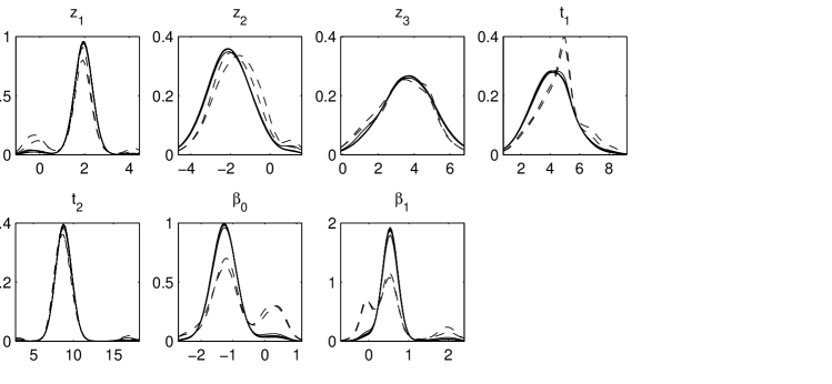
Figure 2: The posterior mean marginal densities of each parameters in the CALGB example. The lines indicated a group in CALGB 8881 (solid line) and CALGB 9160 (dashed line).

The results of the analysis are illustrated in Figure 2 which shows the posterior mean marginal density of each parameter. The results within each study are very similar with the main difference occurring between the two studies. All densities are very similar for the parameters $z_{1}$, $z_{2}$, $z_{3}$ and $t_{2}$. There is a slight difference in the distribution for $t_{1}$ but much bigger differences for parameters $\beta_{0}$ and $\beta_{1}$. The results for CALGB 8881 are unimodal whereas CALGB9160 includes additional modes at 0.5 for $\beta_{0}$ and $-0.5$ and 2 for $\beta_{1}$. Figure 3 shows the posterior mean joint density of $\beta_{0}$ and $\beta_{1}$ which shows a bimodal distribution for CALGB9160 with one mode at roughly $(-1.5,0.5)$ (which is the mode for CALGB8881) and a second mode at roughly $(-0.5,0)$. This suggests that CALGB9160 may contains two groups who responded differently. The posterior median of $\phi$ was 1.03 with a 95% highest posterior density region of $(0.46,2.36)$.

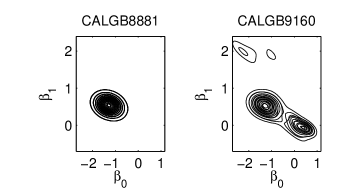
Figure 3: The posterior mean joint densities of $\beta_{0}$ and $\beta_{1}$ in the CALGB example for the groups in CALGB 8881 and CALGB 9160.

7 Discussion

The modelling of dependent random measures has been an extremely active area of research for the past fifteen years beginning with the seminal work of MacEachern [34]. Much of the work has concentrated on dependent random probability measures with several general approaches developed in the literature. Using the notation of (1.1), initial work considered approaches where $w_{i}(x)=w_{i}$ and dependence is modelled through the atom location $\theta_{i}(x)$. This implies that cluster sizes will be similar for all values of $x$ and so leads to a specific form of dependence. Alternatively, many authors used $\theta_{i}(x)=\theta$ for all $x$ with dependence modelled through the weights; often using a stick-breaking construction where $w_{i}(x)=V_{i}(x)\prod_{j<i}(1-V_{j}(x))$, see e.g. [9] for a review. This usually leads to computationally tractable methods which either extend random truncation methods such as retrospective sampling [38] or slice sampling [24], or develop truncation ideas for Dirichlet process mixtures [22]. However, stick-breaking approaches have some limitations for modelling. The construction implies a stochastic ordering so that $w_{1}(x)$ will tend to be the largest weight for all $x$. This can be inappropriate for some regression problems where we would like different component to have large weights for different values of $x$. The correlation is usually built on $V_{j}(x)$ and so $w_{i}(x)$ is a non-linear function of many correlated processes. This can lead to a dependence structure on $w_{i}(x)$ which is hard to interpret. Analytical results such as generalizations of the exchangeable partition probability function are usually impossible to derive for these priors. These methods can often be applied to problems where $\mathcal{X}$ is continuous or discrete. Other priors are restricted to a discrete $\mathcal{X}$. One approach builds a hierarchy of nonparametric processes (see [46] for a review) leading from the seminal work of [47] on hierarchical Dirichlet process (HDP). For example, a two level hierarchical model could be constructed by assuming that the distributions for each group are conditionally independent draws from a nonparametric prior which is centred on a process which is itself given a nonparametric prior. This leads to the same correlation a priori between the distribution for each value in $\mathcal{X}$ (although, more complicated hierarchical structures could be introduced to allow different correlation within subsets of $\mathcal{X}$). Posterior simulation is usually implemented using the Chinese restaurant franchise algorithm.

The CoRM in its most general form is very flexible and allows both hierarchical and regression models. Normalized compound random measures includes many previously described priors which makes the links between these priors clearer. This paper has concentrated on priors where the dimensions of the scores are independent. The tractability of these measures allows their properties to be derived and we concentrate on the class where the dimension of the scores are gamma distributed. If the moment generating function of the marginal score distributions is available analytically, posterior computation for NCoRM mixture model can be carried out using an augmented Pólya urn scheme or a slice sampler and several useful analytical expressions can be derived. This restricts modelling to hierarchical type structures. More general, CoRM-type models where the scores are given by a regression are discussed by [42] who use a truncation of the infinite dimensional parameter and variational Bayes to make inference. In future work, we intend to extend both the Pólya urn scheme and slice sampler to regression models.

The compound random measure is defined using a completely random measure and a finite dimensional score distribution. For a given marginal process, the dependence between the distributions is controlled by the choice of finite dimensional score distribution. In this paper, we have concentrated on the case where the scores are independent and gamma distributed. This allows the dependence between the measures in different dimensions to be modelled by the shape parameter of the gamma distribution. In this case, we show how compound random measures can be constructed with gamma, $\sigma$-stable and generalized gamma process marginals. Importantly, the modelling of dependence between random measures can be achieved by the modelling of dependence between random variables and so greatly reduces the difficulty of specifying a prior for a particular problem. Future work will consider studying these classes of compound random measures.

Appendix A Levy Copulas

For the sake of illustration, we consider the 2-dimensional case.

Definition 5.

A Lévy copula is a function $C:[0,\infty]^{2}\rightarrow[0,\infty]$ such that

1. $C(y_{1},0)=C(0,y_{2})=0$ for any positive $y_{1}$ and $y_{2}$,

2. C has uniform margins, i.e. $C(y_{1},\infty)=y_{1}$ and $C(\infty,y_{2})=y_{2}$,

3. for all $y_{1}<z_{1}$ and $y_{2}<z_{2}$, $C(y_{1},y_{2})+C(z_{1},z_{2})-C(y_{1},z_{2})-C(y_{2},z_{1})\geq 0$.

The definition in higher dimension is analogous (see [6]). Let $U_{i}(x):=\int_{x}^{\infty}\nu_{i}(s)\,ds$ be the $i$–th marginal tail integral associated with $\nu_{i}$. If both the copula $C$ and the marginal tail integrals are sufficiently smooth, then

$$\rho_{2}(s_{1},s_{2})=\frac{\partial^{2}\,C(y_{1},y_{2})}{\partial y_{1}\partial y_{2}}\,\bigg{|}_{y_{1}=U_{1}(s_{1}),y_{2}=U_{2}(s_{2})}\>\nu_{1}(s_{1})\nu_{2}(s_{2}).$$

A wide range of dependence structures can be induced through Lévy copulas. For example the independence case, i.e. $\int_{A\times B}\rho_{2}(s_{1},s_{2})\,ds_{1}\,ds_{2}=\int_{A}\nu_{1}(s_{1})\,ds_{1}+\int_{B}\nu_{2}(s_{2})\,ds_{2}$ for any $A$ and $B$ in $\mathcal{B}(\mathbb{R}^{+})$, corresponds to the Lévy copula

$$C_{\perp}(y_{1},y_{2})=y_{1}\mathbb{I}_{\{\infty\}}(y_{2})+y_{2}\mathbb{I}_{\{\infty\}}(y_{1}).$$

where $\mathbb{I}_{A}$ is the indicator function of the set $A$. On the other hand, the case of completely dependent CRMs corresponds to

$$C_{\parallel}(y_{1},y_{2})=\min\{y_{1},y_{2}\}$$

which yields a vector $(\tilde{\mu}_{1},\tilde{\mu}_{2})$ such that for any $x$ and $y$ in $\mathbb{X}$ either $\tilde{\mu}_{i}(\{x\})<\tilde{\mu}_{i}(\{y\})$ or $\tilde{\mu}_{i}(\{x\})>\tilde{\mu}_{i}(\{y\})$, for $i=1,2$, almost surely. Intermediate cases, between these two extremes, can be detected, for example, by relying on the Lévy-Clayton copula defined by

$$C_{\gamma}(y_{1},y_{2})=(y_{1}^{-\gamma}+y_{2}^{-\gamma})^{-\frac{1}{\gamma}}\qquad\gamma>0.$$ (A.1)

with the parameter $\theta$ regulating the degree of dependence. It can be seen that $\lim_{\gamma\rightarrow 0}C_{\gamma}=C_{\perp}$ and $\lim_{\gamma\rightarrow\infty}C_{\gamma}=C_{\parallel}.$

Appendix B Additional Results

In the following theorem, the derivatives (up to a constant) of the Laplace exponent of a Compound random measure are provided.

Theorem B.1.

Let

$$g_{\rho}(q_{1},\dots,q_{d};\bm{\lambda})=\int_{(0,\infty)^{d}}s_{1}^{q_{1}}\cdots s_{d}^{q_{d}}e^{-\psi_{\rho,d}(\bm{\lambda})}\rho_{d}(s_{1},\dots,s_{d})d\bm{s}.$$ (B.1)

Then,

$$g_{\rho}(q_{1},\dots,q_{d};\bm{\lambda})=(-1)^{q_{1}+\cdots+q_{d}}\int\nu^{\star}(z)\left(\prod_{j=1}^{d}\frac{\partial^{q_{i}}}{\partial\lambda_{i}^{q_{i}}}M_{z}^{f}(-\lambda_{i})\right)dz.$$

Proof.

$$\begin{split}g_{\rho}(q_{1},\dots,q_{d};\bm{\lambda})&=\int_{(0,\infty)^{d}}s_{1}^{q_{1}}\cdots s_{d}^{q_{d}}e^{-\lambda_{1}s_{1}-\cdots-\lambda_{d}s_{d}}\rho_{d}(s_{1},\dots,s_{d})ds_{1}\cdots ds_{d}\\ &=\int\nu^{\star}(z)\left(\prod_{j=1}^{d}\int s_{j}^{q_{1}}e^{-\lambda_{j}s_{j}}z^{-1}f(s_{j}/z)ds_{j}\right)dz\\ &=\int\nu^{\star}(z)\left(\prod_{j=1}^{d}(-1)^{q_{j}}\frac{\partial^{q_{j}}}{\partial\lambda_{j}^{q_{j}}}\left(\int e^{-\lambda_{j}s_{j}}z^{-1}f(s_{j}/z)ds_{j}\right)\right)dz\\ &=(-1)^{q_{1}+\cdots+q_{d}}\int\nu^{\star}(z)\left(\prod_{j=1}^{d}\frac{\partial^{q_{j}}}{\partial\lambda_{j}^{q_{j}}}M_{z}^{f}(-\lambda_{j})\right)dz\\ \end{split}$$

∎

Appendix C Proofs

Proof of Theorem 3.1

$$\begin{split}\psi_{\rho,d}(\lambda_{1},\dots,\lambda_{d})&=\int_{[0,+\infty]^{d}}(1-e^{-\lambda_{1}s_{1}-\cdots-\lambda_{d}s_{d}})\rho_{d}(s_{1},\dots,s_{d})ds_{1}\dots ds_{d}\\ &=\int_{[0,+\infty]^{d}}(1-e^{-\lambda_{1}s_{1}-\cdots-\lambda_{d}s_{d}})\int z^{-d}\prod_{j=1}^{d}f(s_{j}/z)\nu^{\star}(z)\,dzds_{1}\dots ds_{d}\\ &=\int z^{-d}\left(\int_{[0,+\infty]^{d}}(1-e^{-\lambda_{1}s_{1}-\cdots-\lambda_{d}s_{d}})\prod_{j=1}^{d}f(s_{j}/z)ds_{1}\dots ds_{d}\right)\nu^{\star}(z)\,dz\\ &=\int z^{-d}\left(\int_{[0,+\infty]^{d}}\left(\prod_{j=1}^{d}f(s_{j}/z)-e^{-\lambda_{1}s_{1}-\cdots-\lambda_{d}s_{d}}\prod_{j=1}^{d}f(s_{j}/z)\right)ds_{1}\dots ds_{d}\right)\nu^{\star}(z)\,dz\\ &=\int z^{-d}\left(z^{d}-\int_{[0,+\infty]^{d}}\prod_{j=1}^{d}e^{-\lambda_{j}s_{j}}f(s_{j}/z)ds_{1}\dots ds_{d}\right)\nu^{\star}(z)\,dz\\ &=\int z^{-d}\left(z^{d}-\prod_{j=1}^{d}\int_{[0,+\infty]}e^{-\lambda_{j}s_{j}}f(s_{j}/z)ds_{j}\right)\nu^{\star}(z)\,dz\\ &=\int z^{-d}\left(z^{d}-\prod_{j=1}^{d}zM_{z}^{f}(-\lambda_{j})\right)\nu^{\star}(z)\,dz\\ &=\int\left(1-\prod_{j=1}^{d}M_{z}^{f}(-\lambda_{j})\right)\nu^{\star}(z)\,dz\end{split}$$

Proof of Theorem 4.1

Gamma marginals. From 3.383.4 of [16] follows the thesis. Indeed,

$$\begin{split}\rho_{d}(s_{1},\dots,s_{d})&=\int\nu^{\star}(z)z^{-d}\prod_{j=1}^{d}f(s_{j}/z)dz\\ &=\int_{0}^{1}z^{-1}(1-z)^{\phi-1}z^{-d}\frac{\left(\prod_{j=1}^{d}s_{j}\right)^{\phi-1}}{[\Gamma(\phi)]^{d}}z^{-d\phi+d}e^{-\frac{\bm{|s|}}{z}}dz\\ &=\frac{\left(\prod_{j=1}^{d}s_{j}\right)^{\phi-1}}{[\Gamma(\phi)]^{d}}\int_{0}^{1}z^{-d\phi-1}(1-z)^{\phi-1}e^{-\frac{|\bm{s}|}{z}}dz\\ &=\frac{\left(\prod_{j=1}^{d}s_{j}\right)^{\phi-1}}{[\Gamma(\phi)]^{d}}\int_{1}^{+\infty}t^{(d-1)\phi+1}\left(t-1\right)^{\phi-1}e^{-|s|t}dt\\ &=\frac{\left(\prod_{j=1}^{d}s_{j}\right)^{\phi-1}}{[\Gamma(\phi)]^{d-1}}|\bm{s}|^{-\frac{d\phi+1}{2}}e^{-\frac{|\bm{s}|}{2}}W_{\frac{(d-2)\phi+1}{2},-\frac{d\phi}{2}}(|\bm{s}|)\end{split}$$

$\sigma$-stable marginals. In this case,

$$\begin{split}\rho_{d}(s_{1},\dots,s_{d})&=\int_{0}^{+\infty}z^{-\sigma-1}\frac{\Gamma(\phi)}{\Gamma(\sigma)\Gamma(1-\sigma)}z^{-d}\frac{\left(\prod_{j=1}^{d}s_{j}\right)^{\phi-1}}{[\Gamma(\phi)]^{d}}z^{-d\phi+d}e^{-\frac{\bm{|s|}}{z}}dz\\ &=\frac{1}{\Gamma(\sigma)\Gamma(1-\sigma)}\frac{\left(\prod_{j=1}^{d}s_{i}\right)^{\phi-1}}{[\Gamma(\phi)]^{d-1}}\int_{0}^{+\infty}z^{-d\phi-\sigma-1}e^{-\frac{\bm{|s|}}{z}}dz\\ &=\frac{\Gamma(\sigma+d\phi)}{\Gamma(\sigma)\Gamma(1-\sigma)}\frac{\left(\prod_{j=1}^{d}s_{j}\right)^{\phi-1}}{[\Gamma(\phi)]^{d-1}}\bm{|s|}^{-\sigma-d\phi}\end{split}$$

Proof of Corollary 4.1

Gamma marginals. First of all, note that the Whittaker function could be expressed in terms of a Kummer confluent hypergeometric function,

$$W_{\frac{(d-2)\phi+1}{2},-\frac{d\phi}{2}}(|\bm{s}|)=e^{-\frac{|\bm{s}|}{2}}|\bm{s}|^{-\frac{d\phi-1}{2}}U(-(d-1)\phi,-d\phi+1,|\bm{s}|)$$

and thus

$$\rho_{d}(s_{1},\dots,s_{d})=\frac{\left(\prod_{i=1}^{d}s_{i}\right)^{\phi-1}}{[\Gamma(\phi)]^{d-1}}|\bm{s}|^{-d\phi}e^{-|\bm{s}|}U(-(d-1)\phi,-d\phi+1,|\bm{s}|)$$

In the special case of $\phi=1$, we get the following multivariate Lévy intensity

$$\rho_{d}(s_{1},\dots,s_{d})=|\bm{s}|^{-d}e^{-|\bm{s}|}U(-d+1,-d+1,|\bm{s}|)$$

and from 13.2.7 of [36]

$$\begin{split}\rho_{d}(s_{1},\dots,s_{d})&=|\bm{s}|^{-d}e^{-|\bm{s}|}(-1)^{d-1}\sum_{j=0}^{d-1}\binom{d-1}{j}(-1)^{j}(-d+1+j)_{d-1-j}|\bm{s}|^{j}\\ &=|\bm{s}|^{-d}e^{-|\bm{s}|}\sum_{j=0}^{d-1}\binom{d-1}{j}j!|\bm{s}|^{d-1-j}\\ &=\sum_{j=0}^{d-1}\frac{(d-1)!}{(d-1-j)!}|\bm{s}|^{-j-1}e^{-|\bm{s}|}\\ \end{split}$$

$\sigma$-stable marginals. The second part of the proof is straightforward and doesn’t require additional algebra.

Proof of Theorem 4.2

From Equation (3.6) it follows

$$\psi_{\rho,d}(\bm{\tilde{\lambda}},\bm{n})=\int\left(1-\prod_{i=1}^{l}\frac{1}{(1+z\tilde{\lambda}_{i})^{n_{i}\phi}}\right)\nu^{\star}(z)dz$$

since $M_{z}^{f}(-\tilde{\lambda}_{i})=\frac{1}{(1+z\tilde{\lambda}_{i})^{\phi}}$ under the hypothesis of independent Gamma distributed scores. The conclusion follows by noting that $\frac{\partial^{(n_{i}-1)\phi}}{\partial^{(n_{i}-1)\phi}\tilde{\lambda}_{i}}(\tilde{\lambda}_{i}^{n_{i}\phi-1})=\frac{\Gamma(n_{i}\phi)}{\Gamma(\phi)}\tilde{\lambda}_{i}^{\phi-1}$ and

$$\frac{\partial^{(n_{i}-1)\phi}}{\partial^{(n_{i}-1)\phi}\tilde{\lambda}_{i}}\left(\frac{\tilde{\lambda}_{i}^{n_{i}\phi-1}}{(1+z\tilde{\lambda}_{i})^{\phi}}\right)=\frac{\Gamma(n_{i}\phi)}{\Gamma(\phi)}\frac{\tilde{\lambda}_{i}^{\phi-1}}{(1+z\tilde{\lambda}_{i})^{n_{i}\phi}}$$

The last equality follows from a simple application of the Leibniz’s formula, indeed

$$\begin{split}\frac{\partial^{(n_{i}-1)\phi}}{\partial^{(n_{i}-1)\phi}\tilde{\lambda}_{i}}\left(\frac{\tilde{\lambda}_{i}^{n_{i}\phi-1}}{(1+z\tilde{\lambda}_{i})^{\phi}}\right)&=\sum_{j=0}^{(n_{i}-1)\phi}\binom{(n_{i}-1)\phi}{j}\frac{(j+\phi-1)!}{(\phi-1)!}\frac{(-1)^{j}z^{j}}{(1+z\tilde{\lambda}_{i})^{j+\phi}}\frac{(n_{i}\phi-1)!}{(j+\phi-1)!}\tilde{\lambda}_{i}^{j+\phi-1}\\ &=\frac{\Gamma(n_{i}\phi)}{\Gamma(\phi)}\frac{\tilde{\lambda}_{i}^{\phi-1}}{(1+z\tilde{\lambda}_{i})^{\phi}}\sum_{j=0}^{(n_{i}-1)\phi}\binom{(n_{i}-1)\phi}{j}\left(\frac{-z\tilde{\lambda}_{i}}{1+z\tilde{\lambda}_{i}}\right)^{j}\\ &=\frac{\Gamma(n_{i}\phi)}{\Gamma(\phi)}\frac{\tilde{\lambda}_{i}^{\phi-1}}{(1+z\tilde{\lambda}_{i})^{\phi}}\left(\frac{-z\tilde{\lambda}_{i}}{1+z\tilde{\lambda}_{i}}+1\right)^{(n_{i}-1)\phi}\\ &=\frac{\Gamma(n_{i}\phi)}{\Gamma(\phi)}\frac{\tilde{\lambda}_{i}^{\phi-1}}{(1+z\tilde{\lambda}_{i})^{n_{i}\phi}}\\ \end{split}$$

Thus,

$$\begin{split}\psi_{\rho,d}(\bm{\tilde{\lambda}},\bm{n})&=\int\left(1-\prod_{i=1}^{l}\frac{1}{(1+z\tilde{\lambda}_{i})^{n_{i}\phi}}\right)\nu^{\star}(z)dz\\ &=\frac{1}{\prod_{i=1}^{l}\tilde{\lambda}_{i}^{\phi-1}}\int\left(\prod_{i=1}^{l}\tilde{\lambda}_{i}^{\phi-1}-\prod_{i=1}^{l}\frac{\tilde{\lambda}_{i}^{\phi-1}}{(1+z\tilde{\lambda}_{i})^{n_{i}\phi}}\right)\nu^{\star}(z)dz\\ &=\frac{[\Gamma(\phi)]^{l}}{\prod_{i=1}^{l}[\tilde{\lambda}_{i}^{\phi-1}\Gamma(n_{i}\phi)]}\left(\prod_{i=1}^{l}\frac{\partial^{(n_{i}-1)\phi}}{\partial^{(n_{i}-1)\phi}\tilde{\lambda}_{i}}\right)\int\left(\prod_{i=1}^{l}\tilde{\lambda}_{i}^{n_{i}\phi-1}-\prod_{i=1}^{l}\frac{\tilde{\lambda}_{i}^{n_{i}\phi-1}}{(1+z\tilde{\lambda}_{i})^{\phi}}\right)\nu^{\star}(z)dz\\ &=\frac{[\Gamma(\phi)]^{l}}{\prod_{i=1}^{l}[\tilde{\lambda}_{i}^{\phi-1}\Gamma(n_{i}\phi)]}\left(\prod_{i=1}^{l}\frac{\partial^{(n_{i}-1)\phi}}{\partial^{(n_{i}-1)\phi}\tilde{\lambda}_{i}}\right)\left(\Upsilon^{\phi}_{l}(\bm{\tilde{\lambda}})\prod_{i=1}^{l}\tilde{\lambda}_{i}^{n_{i}\phi-1}\right)\\ \end{split}$$

Proof of Theorem 4.3

Let

$$B_{\phi,l}=\{\bm{k}^{*}\in\{0,1,\ldots,\phi\}^{l}:\>|\bm{k}^{*}|=\phi\}\qquad\phi\geq j.$$

First of all, note that

$$\sum_{i=1}^{l}a_{i}(\bm{\tilde{\lambda}})=1$$

and

$$\prod_{i=1}^{l}\frac{1}{(1+z\tilde{\lambda}_{i})}=\sum_{i=1}^{l}\frac{a_{i}(\bm{\tilde{\lambda}})}{(1+z\tilde{\lambda}_{i})}$$

Thus,

$$\begin{split}\Upsilon_{l}^{\phi}(\bm{\tilde{\lambda}})&=\int\left[\left(\sum_{i=1}^{l}a_{i}(\bm{\tilde{\lambda}})\right)^{\phi}-\left(\sum_{i=1}^{l}\frac{a_{i}(\bm{\tilde{\lambda}})}{(1+z\tilde{\lambda}_{i})}\right)^{\phi}\right]\nu^{\star}(z)dz\\ &=\sum_{\bm{k}^{*}\in B_{\phi,l}}\binom{\phi}{k_{1}^{*},\cdots,k_{l}^{*}}a_{1}^{k_{1}^{*}}(\bm{\tilde{\lambda}})\cdots a_{l}^{k_{l}^{*}}(\bm{\tilde{\lambda}})I(k_{1}^{*},\dots,k_{l}^{*};\bm{\tilde{\lambda}})\\ \end{split}$$

where

$$I(k_{1}^{*},\dots,k_{l}^{*};\bm{\tilde{\lambda}})=\int\left(1-\prod_{i=1}^{l}\frac{1}{(1+z\tilde{\lambda}_{i})^{k_{i}^{*}}}\right)\nu^{\star}(z)dz$$

Since some of the $k^{*}$’s could be zero then some terms could disappear in the expression above. For this reason, it’s more convenient to write $\Upsilon_{l}^{\phi}(\bm{\tilde{\lambda}})$ as a sum over the set $A_{\phi,j}$ instead of a sum over $B_{\phi,l}$. Thus,

$$\begin{split}\Upsilon_{l}^{\phi}(\bm{\tilde{\lambda}})&=\sum_{j=1}^{l}\sum_{\bm{k}\in A_{\phi,j}}\binom{\phi}{k_{1},\cdots,k_{j}}\sum_{0<i_{1}<i_{2}<\cdots<i_{j}\leq l}a_{i_{1}}^{k_{1}}(\bm{\tilde{\lambda}})\cdots a_{i_{j}}^{k_{j}}(\bm{\tilde{\lambda}})C(i_{1},\dots,i_{j};\bm{k};\bm{\tilde{\lambda}})\\ \end{split}$$

where

$$C(i_{1},\dots,i_{j};\bm{k};\bm{\tilde{\lambda}})=\int\left(1-\prod_{h=1}^{j}\frac{1}{(1+z\tilde{\lambda}_{i_{h}})^{k_{h}}}\right)\nu^{\star}(z)dz$$

If $j>\phi$ then $A_{\phi,j}$ is the empty set. Thus we can resort the above sum as

$$\begin{split}\Upsilon_{l}^{\phi}(\bm{\tilde{\lambda}})&=\sum_{j=1}^{\phi}\sum_{\bm{k}\in A_{\phi,j}}\binom{\phi}{k_{1},\cdots,k_{j}}\sum_{0<i_{1}<i_{2}<\cdots<i_{j}\leq l}a_{i_{1}}^{k_{1}}(\bm{\tilde{\lambda}})\cdots a_{i_{j}}^{k_{j}}(\bm{\tilde{\lambda}})C(i_{1},\dots,i_{j};\bm{k};\bm{\tilde{\lambda}})\\ \end{split}$$

Let $|\bm{y}|_{\bm{i}}^{j}=y_{i_{1}}+\cdots+y_{i_{j}}$. Note that

$$\begin{split}\int\nu^{\star}(z)dz&=\int\int_{[0,+\infty]^{j}}\prod_{h=1}^{j}\frac{z^{-k_{h}}}{\Gamma(k_{h})}y_{i_{h}}^{k_{h}-1}e^{-\frac{y_{i_{h}}}{z}}d\bm{y}\nu^{\star}(z)dz\\ &=\int_{[0,+\infty]^{j}}\frac{\Gamma(\phi)}{\left(|\bm{y}|_{\bm{i}}^{j}\right)^{\phi-1}}\left(\prod_{h=1}^{j}\frac{y_{i_{h}}^{k_{h}-1}}{\Gamma(k_{h})}\right)\int\frac{\left(|\bm{y}|_{\bm{i}}^{j}\right)^{\phi-1}}{z^{\phi}\Gamma(\phi)}e^{-\frac{|\bm{y}|_{\bm{i}}^{j}}{z}}\nu^{\star}(z)dzd\bm{y}\\ &=\int_{[0,+\infty]^{j}}\frac{\Gamma(\phi)}{\left(|\bm{y}|_{\bm{i}}^{j}\right)^{\phi-1}}\left(\prod_{h=1}^{j}\frac{y_{i_{h}}^{k_{h}-1}}{\Gamma(k_{h})}\right)\nu(|\bm{y}|_{\bm{i}}^{j})d\bm{y}\\ \\ \end{split}$$

In a similar fashion,

$$\begin{split}\int\left(\prod_{h=1}^{j}\frac{1}{(1+z\tilde{\lambda}_{i_{h}})^{k_{h}}}\right)\nu^{\star}(z)dz&=\int_{[0,+\infty]^{j}}\frac{\Gamma(\phi)e^{-\sum_{h=1}^{j}\tilde{\lambda}_{i_{h}}y_{i_{h}}}}{\left(|\bm{y}|_{\bm{i}}^{j}\right)^{\phi-1}}\left(\prod_{h=1}^{j}\frac{y_{i_{h}}^{k_{h}-1}}{\Gamma(k_{h})}\right)\nu(|\bm{y}|_{\bm{i}}^{j})d\bm{y}\\ \\ \end{split}$$

and thus,

$$C(i_{1},\dots,i_{j};\bm{k};\bm{\tilde{\lambda}})=\int_{[0,+\infty]^{j}}\left(1-e^{-\sum_{h=1}^{j}\tilde{\lambda}_{i_{h}}y_{i_{h}}}\right)\frac{\Gamma(\phi)}{\left(|\bm{y}|_{\bm{i}}^{j}\right)^{\phi-1}}\left(\prod_{h=1}^{j}\frac{y_{i_{h}}^{k_{h}-1}}{\Gamma(k_{h})}\right)\nu(|\bm{y}|_{\bm{i}}^{j})d\bm{y}$$

The change of variables $\rho=|\bm{y}|_{\bm{i}}^{j}$ and $y_{i_{h}}=\rho z_{h}$, $h=1,\dots,j-1$ leads to

$$\begin{split}C(i_{1},\dots,i_{j};\bm{k};\bm{\tilde{\lambda}})&=\int_{\Delta_{j-1}}\left(\Gamma(\phi)\prod_{h=1}^{j}\frac{z_{h}^{k_{h}-1}}{\Gamma(k_{h})}\right)\int_{0}^{+\infty}\left(1-e^{-\rho\Lambda(\bm{\tilde{\lambda}},\bm{z})}\right)\nu(\rho)d\rho d\bm{z}\\ &=\int_{\Delta_{j-1}}\Gamma(\phi)\left((1-\sum_{h=1}^{j-1}z_{h})^{k_{j}}\prod_{h=1}^{j-1}\frac{z_{h}^{k_{h}-1}}{\Gamma(k_{h})}\right)\psi\left(\Lambda(\bm{\tilde{\lambda}},\bm{z})\right)d\bm{z}\end{split}$$

Proof of Theorem 4.4

Let $U(x)=\int_{x}^{+\infty}\nu(x)dx$ be the tail integral of the marginal Lévy intensity and let

$$U(x_{1},\dots,x_{d})=\int_{x_{1}}\dots\int_{x_{d}}\nu(s_{1},\dots,s_{d})ds_{1}\cdots ds_{d}.$$

From Theorem 5.3 in Cont and Tankov, exists only one copula C such that

$$U(x_{1},\dots,x_{d})=C(U(x_{1}),\dots,U(x_{d})).$$

It’s easy to see that

$$U(x_{1},\dots,x_{d})=\int\nu^{\star}(z)\prod_{j=1}^{d}(1-F(z^{-1}x_{j}))dz$$

and this proves the thesis.

Proof of Theorem 4.5

In a similar fashion of [29], it’s easy to see that

$$\mathbb{E}\left[\prod_{i=1}^{d}\{\tilde{\mu}_{i}(A)\}^{q_{i}}\right]=e^{-\alpha(A)\psi(0,...,0)}\,q_{1}!\cdots q_{d}!\>\sum_{k=1}^{\mid\bm{q}\mid}[\alpha(A)]^{k}\>\times\>$$

$$\hskip 85.35826pt\times\sum_{j=1}^{\mid\bm{q}\mid}\>\sum_{p_{j}(\bm{q},k)}\>\prod_{i=1}^{j}\frac{1}{\eta_{i}!(s_{1,i}!\cdots s_{d,i}!)^{\eta_{i}}}\left(g_{\nu}(s_{1,i},\dots,s_{d,i},0,\dots,0)\right)^{\eta_{i}}$$

In the gamma case, it’s easy to see that $\psi(0,...,0)=0$ and

$$g_{\nu}(s_{1,i},\dots,s_{d,i},0,\dots,0)=\int\nu^{\star}(z)\prod_{j=1}^{d}(\phi)_{s_{j,i}}z^{s_{j,i}}dz$$

and this concludes the proof.

Appendix D Additional Details of Computational Methods

In the update of $u$ in the Gibbs sampler, it is necessary to sample from the density proportional to simulated from the density of $z$ proportional to

$$\nu^{\star}(z)\prod_{j=1}^{d}\int\exp\left\{-v_{j}m_{j}z\right\}\,f(m_{j})\,dm_{j},\qquad\kappa^{\star}<z<\kappa.$$

If a NCoRM with a $\mbox{Ga}(\phi,1)$ score distribution and Dirichlet process marginals is used, this density is proportional to

$$z^{-1}(1-z)^{\phi-1}\prod_{j=1}^{d}(1+v_{i}z)^{-\phi},\qquad\kappa^{\star}<z<\kappa.$$

A rejection sampler is used with rejection envelope proportional to $z^{-1}(1-z)^{\phi-1},\ \kappa^{\star}<z<\kappa$. The acceptance probability is

$$\prod_{j=1}^{d}\left(\frac{1+v_{j}\kappa^{\star}}{1+v_{j}z}\right)^{\phi}.$$

This rejection envelope is non-standard and can be sampled using a rejection sampler with the envelope

$$g(z)=\left\{\begin{array}[]{rll}(1-z)^{\phi-1},&\kappa^{\star}<z<\kappa,&\mbox{if }\phi<1\\ z^{-1},&\kappa^{\star}<z<\kappa,&\mbox{if }\phi>1\end{array}\right..$$

If a NCoRM with a $\mbox{Ga}(\phi,1)$ score distribution and normalized generalized gamma process marginals with $a=1$ is used, this density is proportional to

$$z^{-1-\sigma}(1-z)^{\sigma+\phi-1}\prod_{j=1}^{d}(1+v_{i}z)^{-\phi},\qquad\kappa^{\star}<z<\kappa.$$

A rejection sampler is used with rejection envelope proportional to $z^{-1-\sigma}(1-z)^{\sigma+\phi-1},\ \kappa^{\star}<z<\kappa$. The acceptance probability is

$$\prod_{j=1}^{d}\left(\frac{1+v_{j}\kappa^{\star}}{1+v_{j}z}\right)^{\phi}.$$

This rejection envelope is non-standard and can be sampled using a rejection sampler with the envelope

$$g(z)=\left\{\begin{array}[]{rll}(1-z)^{\sigma+\phi-1},&\kappa^{\star}<z<\kappa,&\mbox{if }\sigma+\phi<1\\ z^{-1-\sigma},&\kappa^{\star}<z<\kappa,&\mbox{if }\sigma+\phi>1\end{array}\right..$$

References

• AtchadΓ© and Rosenthal [2005] Y. F. AtchadΓ© and J. S. Rosenthal (2005). On Adaptive Markov Chain Monte Carlo Algorithms, Bernoulli, 11, 815–828.
• Bassetti, Casarin and Leisen [2014] F. Bassetti, R. Casarin and F. Leisen (2014). Beta-Product dependent Pitman-Yor Processes for Bayesian inference. Journal of Econometrics. 180, 49–72.
• Budman et al. [1998] D. Budman, G. Rosner, S. Lichtman, A. Miller, M. Ratain and R. Schilsky (1998). A randomized trial of wr-2721 (amifostine) as a chemoprotective agent in combination with high-dose cyclophosphamide and molgramostim (GM-CSG). Cancer Therapeutics, 1, 164–167
• Chen et al [2013] C. Chen, V. A. Rao, W. Buntine and Y. W. Teh (2013). Dependent Normalized Random Measures, Proceedings of the International Conference on Machine Learning.
• Constantine and Savits [1996] G. M. Constantines and T. H. Savits (1996). A multivariate version of the FaaΒ diΒ Bruno formula. Trans. Amer. Math. Soc. 348, 503–520.
• Cont and Tankov [2004] R. Cont and P. Tankov (2004). Financial modelling with jump processes. Chapman & Hall/CRC, Boca Raton, FL.
• Daley and Vere-Jones [2003] D. J. Daley and D. Vere-Jones (2003). An introduction to the theory of point processes. Vol. 1. Springer, New York.
• De Iorio et al. [2004] M. De Iorio, P. MΓΌller, G. L. Rosner, S. N. MacEachern (2004). An ANOVA model for dependent random measures. J. Amer. Statist. Assoc. 99, 205–215.
• Dunson [2010] D. B. Dunson (2010). Nonparametric Bayes applications to biostatistics. In N. L. Hjort, C. C. Holmes, P. MΓΌller and S. G. Walker, editors, Bayesian Nonparametrics, Cambridge University Press.
• Epifani and Lijoi [2010] I. Epifani and A. Lijoi (2010). Nonparametric priors for vectors of survival functions. Statistica Sinica 20, 1455–1484.
• Favaro et al. [2009] S. Favaro, A. Lijoi, R.H. Mena and I. PrΓΌnster (2009). Bayesian nonparametric inference for species variety with a two parameter Poisson-Dirichlet process prior. Journal of the Royal Statistical Society Series B, vol. 71, 993–1008.
• Favaro, Lijoi and Pruenster [2012] S. Favaro, A. Lijoi, and I. PrΓΌnster (2012). A new estimator of the discovery probability. Biometrics, vol. 68, pp. 1188–1196.
• Favaro and Teh [2013] S. Favaro and Y. W. Teh (2013). MCMC for Normalized Random Measure Mixture Models. Statistical Science, vol. 28, 335–359.
• Ferguson [1973] T. S. Ferguson (1973). A Bayesian analysis of some nonparametric problems. Ann. Statist. 1, 209–230.
• Foti and Williamson [2012] N. Foti and S. Williamson (2012). Slice sampling normalized kernel-weighted completely random measure mixture models. In Advances in Neural Information Processing Systems 25, (F. Pereira, C. J. C. Burges, L. Bottou and K. Q. Weinberger, Eds.), 2240–2248.
• Gradshtein and Ryzhik [2007] I. S. Gradshteyn and J.M. Ryzhik (2007). Table of Integrals, Series, and Products. 7th Ed. Academic Press, New York.
• Griffin [2011] J. E. Griffin (2011). The Ornstein-Uhlenback Dirichlet process and other time-varying processes for Bayesian nonparametric inference. Journal of Statistical Planning and Inference, 141, 3648–3664.
• Griffin et al. [2013] J. E. Griffin, M. Kolossiatis and M. F. J. Steel (2013). Comparing Distributions By Using Dependent Normalized Random-Measure Mixtures. Journal of the Royal Statistical Society, Series B, 75, 499–529.
• Griffin and Steel [2006] J. E. Griffin and M. F. J. Steel (2006). Order-based dependent Dirichlet processes. Journal of the American Statistical Association 101, 179–194.
• Griffin and Walker [2011] J. E. Griffin and S. G. Walker (2011). Posterior simulation of normalized random measure mixtures. Journal of Computational and Graphical Statistics 20, 241–259.
• Hatjispyrosa et al. [2011] S. J. Hatjispyrosa, T. N. Nicoleris, and S. G. Walker (2011). Dependent mixtures of Dirichlet processes. Computational Statistics and Data Analysis, 55, 2011–2025.
• Ishwaran and James [2001] H. Ishwaran and L. F. James (2001). Gibbs sampling methods for stick-breaking priors. Journal of the American Statistical Association 96, 161–173.
• James et al. [2009] L. F. James, A. Lijoi and I. PrΓΌnster, I. (2009). Posterior Analysis for Normalized Random Measures with Independent Increments, Scandinavian Journal of Statistics, 36, 76–97.
• Kalli et al. [2011] M. Kalli, J. E. Griffin and S. G. Walker (2011). Slice sampling mixture models. Statistics and Computing, 21, 93–105.
• Kingman [1967] J. F. C. Kingman (1967). Completely Random Measures. Pacific Journal of Mathematics, 21, 59–78.
• Kingman [1993] J. F. C. Kingman (1993). Poisson processes. Oxford University Press, Oxford.
• Kolossiatis et al. [2013] M. Kolossiatis, J. E. Griffin, and M. F. J. Steel (2013). On Bayesian nonparametric modelling of two correlated distributions. Statistics and Computing, 23, 1–15.
• Leisen and Lijoi [2011] F. Leisen and A. Lijoi (2011). Vectors of Poisson-Dirichlet processes. J. Multivariate Anal., 102, 482–495.
• Leisen, Lijoi and Spano [2013] F. Leisen, A. Lijoi and D. Spano (2013). A Vector of Dirichlet processes. Electronic Journal of Statistics 7, 62–90.
• Lichtman et al. [1993] S. M. Lichtman, M. J. Ratain, D. A. Echo, G. Rosner, M. J. Egorin, D. R. Budman, N. J. Vogelzang, L. Norton and R. L. Schilsky (1993). Phase I trial and granulocyte-macrophage colony-stimulating factor plus high-dose cyclophosphamide given every 2 weeks: a Cancer and Leukemia Group B study. Journal of the National Cancer Institute, 85, 1319–1326.
• Lijoi and Nipoti [2014] A. Lijoi, and B. Nipoti (2014), β€˜A class of hazard rate mixtures for combining survival data from different experiments’, Journal of the American Statistical Association, 109, 802–814.
• Lijoi, Nipoti and PrΓΌnster [2014a] A. Lijoi, B. Nipoti and I. PrΓΌnster (2014a), β€˜Bayesian inference with dependent normalized completely random measures’, Bernoulli, 20, 1260–1291.
• Lijoi, Nipoti and PrΓΌnster [2014b] A. Lijoi, B. Nipoti and I. PrΓΌnster (2014b), β€˜Dependent mixture models: clustering and borrowing information’, Computational Statistics and Data Analysis, 71, 417–433.
• MacEachern [1999] S. N. MacEachern (1999). Dependent nonparametric processes. In ASA Proceedings of the Section on Bayesian Statistical Science, Alexandria, VA: American Statistical Association.
• MΓΌller et al. [2004] P. MΓΌller, F. Quintana and G. L. Rosner (2004). A method for combining inference across related nonparametric Bayesian models. Journal of the Royal Statistical Society, Series B, 66, 735–749.
• Olver et al. [2010] F. W. J. Olver, D. W. Lozier, R. F. Boisvert and C. W. Clark (2010). Handbook of Mathematical Functions. Cambridge University Press.
• Palla et al. [2014] K. Palla, D. A. Knowles and Z. Ghahramani (2014). A reversible infinite HMM using normalised random measures, Journal of Machine Learning Research, 32.
• Papaspiliopoulos and Roberts [2008] O. Papaspiliopoulos and G. O. Roberts (2008). Retrospective Markov chain Monte Carlo methods for Dirichlet process hierarchical models, Biometrika, 95, 169–186.
• Pitman and Yor [1997] J. Pitman and M. Yor (1997). The two-parameter Poisson-Dirichlet distribution derived from a stable subordinator. Annals of Probability 25, 855–900.
• Pitman [2006] J. Pitman (2006). Combinatorial Stochastic Processes. Ecole d’EtΓ© de ProbabilitΓ©s de Saint-Flour XXXII 2002. Lecture Notes in Mathematics 1875. Springer, Berlin.
• Pitman and Yor [1997] J. Pitman and M. Yor (1997). The two-parameter Poisson-Dirichlet distribution derived from a stable subordinator. Ann. Probab. 25, 855–900.
• Ranganath and Blei [2015] R. Ranganath and D. M. Blei. Correlated Random Measures. arXiv:1507.00720
• Regazzini, Lijoi and PrΓΌnster [2003] E. Regazzini, A. Lijoi and I. PrΓΌnster (2003). Distributional results for means of normalized random measures with independent increments. Ann. Statist. 31, 560–585.
• Sato [1999] K. Sato (1999).LΓ©vy Processes and Infinitely Divisible Distributions. Cambridge University Press.
• Teh and GΓΆrΓΌr [2009] Y. W. Teh and D. GΓΆrΓΌr (2009). Indian Buffet Proceses with Power-law Behavior. In Advances in Neural Information Processing Systems 22 (Y. Bengio, D. Schuurmans, J. D. Lafferty, C. K. I. Williams and A. Culotta, Eds.), 1838–1846.
• Teh and Jordan [2010] Y. W. Teh and M. I. Jordan (2010). Hierarchical Bayesian nonparametric models with applications. In Bayesian nonparametrics (N. L. Hjort, C. C. Holmes, P. MΓΌller and S. G. Walker, Eds.), 158–207, Cambridge University Press, Cambridge.
• Teh et al [2006] Y. W. Teh, M. I. Jordan, M. J. Beal and D. M. Blei (2006). Hierarchical Dirichlet processes. Journal of the American Statistical Association, 101, 1566–1581.
• Yu and Meng [2011] Y. Yu and X.-L. Meng (2011). To Center or Not to Center: That is Not the Question – An Ancillarity-Sufficiency Interweaving Strategy (ASIS) for Boosting MCMC Efficiency. Journal of Computational and Graphical Statistics, vol. 20, 531–570.
• Zhu and Leisen [2014] W. Zhu and F. Leisen (2014). A multivariate extension of a vector of Poisson-Dirichlet processes. To appear in the Journal of Nonparametric Statistics.