The light-front coupled-cluster method applied to $\phi_{1+1}^{4}$ theory

Abstract

We use the light-front coupled-cluster (LFCC) method to compute the odd-parity massive eigenstate of $\phi_{1+1}^{4}$ theory. A standard Fock-space truncation of the eigenstate yields a finite set of linear equations for a finite number of wave functions. The LFCC method replaces Fock-space truncation with a more sophisticated truncation; the eigenvalue problem is reduced to a finite set of nonlinear equations without any restriction on Fock space, but with restrictions on the Fock wave functions. We compare our results with those obtained with a Fock-space truncation.

I Introduction

The nonperturbative solution of quantum field theories in terms of Fock-state wave functions requires new methods that avoid various difficulties. Light-front quantization DLCQreviews is critical for this, because it allows for a well-defined Fock-state expansion of Hamiltonian eigenstates. The calculation of these wave functions is usually done in a truncated Fock space, in order to have a finite number of equations; however, such a truncation brings problems with uncanceled divergences. An alternate truncation that apparently avoids such divergences is made within the light-front coupled-cluster (LFCC) method LFCC .

The LFCC method replaces a Fock-space truncation with a more sophisticated truncation, one that limits the way in which higher Fock-state wave functions are related without completely eliminating any. The light-front Hamiltonian eigenvalue problem is reduced to a finite set of nonlinear equations, rather than the finite linear set obtained from a Fock-space truncation.

Here we consider $\phi^{4}$ theory in 1+1 dimensions as an illustration of the use of the LFCC method LFCCphi4 . We compute the odd-parity massive eigenstate and compare results with those obtained with a Fock-space truncation.

Our light-front coordinates Dirac are defined as $x^{+}=t+z$ for time and $x^{-}=t-z$ for space. The corresponding light-front energy and momentum are $p^{-}=E-p_{z}$ and $p^{+}=E+p_{z}$. The mass-shell condition $p^{2}=m^{2}$ becomes $p^{-}=\frac{m^{2}}{p^{+}}$. The light-front Hamiltonian operator is written as ${\cal P}^{-}$.

II LFCC method

To solve the light-front eigenvalue problem

$${\cal P}^{-}|\psi(P^{+})\rangle=\frac{M^{2}}{P^{+}}|\psi(P^{+})\rangle$$ (1)

without making a Fock-space truncation, we build the eigenstate as

$$|\psi\rangle=\sqrt{Z}e^{T}|\phi\rangle$$ (2)

from a valence state $|\phi\rangle$ and an operator $T$ that increases particle number. The eigenvalue problem can then be written as

$$e^{-T}{\cal P}^{-}e^{T}|\phi\rangle=e^{-T}\frac{M^{2}}{P^{+}}e^{T}|\phi\rangle.$$ (3)

We define an effective Hamiltonian $\overline{{\cal P}^{-}}=e^{-T}{\cal P}^{-}e^{T}$, and the eigenvalue problem becomes $\overline{{\cal P}^{-}}|\phi\rangle=\frac{M^{2}}{P^{+}}|\phi\rangle$, which we project onto the valence and orthogonal sectors

$$P_{v}\overline{{\cal P}^{-}}|\phi\rangle=\frac{M^{2}+P_{\perp}^{2}}{P^{+}}|\phi\rangle,\;\;(1-P_{v})\overline{{\cal P}^{-}}|\phi\rangle=0.$$ (4)

with $P_{v}$ the projection operator. The second (auxiliary) equation determines $T$.

This formulation is exact; however, in general, $T$ contains an infinite number of terms, and the auxiliary equation is really an infinite set of equations. The approximation made is to truncate $T$ and truncate $1-P_{v}$. The effective Hamiltonian can then be constructed from a Baker–Hausdorff expansion $\overline{{\cal P}^{-}}={\cal P}^{-}+[{\cal P}^{-},T]+\frac{1}{2}[[{\cal P}^{-},T],T]+\ldots$, which can be terminated when the increase in particle number matches the truncation of the projection $1-P_{v}$.

III Application to $\phi^{4}$ theory

The Lagrangian for two-dimensional $\phi^{4}$ theory is

$${\cal L}=\frac{1}{2}(\partial_{\mu}\phi)^{2}-\frac{1}{2}\mu^{2}\phi^{2}-\frac{\lambda}{4!}\phi^{4},$$ (5)

where $\mu$ is the mass of the boson and $\lambda$ is the coupling constant. The light-front Hamiltonian density is

$${\cal H}=\frac{1}{2}\mu^{2}\phi^{2}+\frac{\lambda}{4!}\phi^{4}.$$ (6)

The mode expansion for the field at zero light-front time is

$$\phi=\int\frac{dp^{+}}{\sqrt{4\pi p^{+}}}\left\{a(p^{+})e^{-ip^{+}x^{-}/2}+a^{\dagger}(p^{+})e^{ip^{+}x^{-}/2}\right\},$$ (7)

with the modes quantized such that

$$[a(p^{+}),a^{\dagger}(p^{\prime+})]=\delta(p^{+}-p^{\prime+}).$$ (8)

The light-front Hamiltonian is ${\cal P}^{-}={\cal P}^{-}_{11}+{\cal P}^{-}_{13}+{\cal P}^{-}_{31}+{\cal P}^{-}_{22}$, with

$${\cal P}^{-}_{11} = \int dp^{+}\frac{\mu^{2}}{p^{+}}a^{\dagger}(p^{+})a(p^{+}),$$ (9)

$${\cal P}^{-}_{13} = \frac{\lambda}{6}\int\frac{dp_{1}^{+}dp_{2}^{+}dp_{3}^{+}}{4\pi\sqrt{p_{1}^{+}p_{2}^{+}p_{3}^{+}(p_{1}^{+}+p_{2}^{+}+p_{3}^{+})}}a^{\dagger}(p_{1}^{+}+p_{2}^{+}+p_{3}^{+})a(p_{1}^{+})a(p_{2}^{+})a(p_{3}^{+}),$$ (10)

$${\cal P}^{-}_{31} = \frac{\lambda}{6}\int\frac{dp_{1}^{+}dp_{2}^{+}dp_{3}^{+}}{4\pi\sqrt{p_{1}^{+}p_{2}^{+}p_{3}^{+}(p_{1}^{+}+p_{2}^{+}+p_{3}^{+})}}a^{\dagger}(p_{1}^{+})a^{\dagger}(p_{2}^{+})a^{\dagger}(p_{3}^{+})a(p_{1}^{+}+p_{2}^{+}+p_{3}^{+}),$$ (11)

$${\cal P}^{-}_{22} = \frac{\lambda}{4}\int\frac{dp_{1}^{+}dp_{2}^{+}}{4\pi\sqrt{p_{1}^{+}p_{2}^{+}}}\int\frac{dp_{1}^{\prime+}dp_{2}^{\prime+}}{\sqrt{p_{1}^{\prime+}p_{2}^{\prime+}}}\delta(p_{1}^{+}+p_{2}^{+}-p_{1}^{\prime+}-p_{2}^{\prime+})$$

$$\rule{144.54pt}{0.0pt}\times a^{\dagger}(p_{1}^{+})a^{\dagger}(p_{2}^{+})a(p_{1}^{\prime+})a(p_{2}^{\prime+}).$$

The subscripts indicate the number of creation and annihilation operators in each term. Each term changes the number of particles by two or zero, which allows the eigenstates to be classified as either odd or even in the number of constituents.

For simplicity of the illustration, we consider the odd case. The valence state $|\phi\rangle$ is the one-particle state $a^{\dagger}(P^{+})|0\rangle$. The leading contribution to the $T$ operator is

$$T_{2}=\int dp_{1}^{+}dp_{2}^{+}dp_{3}^{+}t_{2}(p_{1}^{+},p_{2}^{+},p_{3}^{+})a^{\dagger}(p_{1}^{+})a^{\dagger}(p_{2}^{+})a^{\dagger}(p_{3}^{+})a(p_{1}^{+}+p_{2}^{+}+p_{3}^{+});$$ (13)

the function $t_{2}$ is symmetric in its arguments. For $T$ truncated to $T_{2}$, the projection $1-P_{v}$ is truncated to projection onto the three-particle state $a^{\dagger}(p_{1}^{+})a^{\dagger}(p_{2}^{+})a^{\dagger}(p_{3}^{+})|0\rangle$.

Given this truncation, the Baker–Hausdorff expansion for $\overline{{\cal P}^{-}}$ generates many terms that do not actually contribute to the valence equation or to the auxiliary equation. A more efficient approach for the construction of these equations is to compute only those matrix elements of $\overline{{\cal P}^{-}}$ that enter into the projections. The valence and auxiliary equations become

$$\langle 0|a(Q^{+})\left({\cal P}^{-}_{11}+{\cal P}^{-}_{13}T_{2}\right)a^{\dagger}(P^{+})|0\rangle=\frac{M^{2}}{P^{+}}\delta(Q^{+}-P^{+}).$$ (14)

and

$$\langle 0|a(q_{1}^{+})a(q_{2}^{+})a(q_{3}^{+})\left(\rule{0.0pt}{14.45377pt}{\cal P}^{-}_{31}+({\cal P}^{-}_{11}+{\cal P}^{-}_{22})T_{2}-T_{2}{\cal P}^{-}_{11}-T_{2}{\cal P}^{-}_{13}T_{2}+\frac{1}{2}{\cal P}^{-}_{13}T_{2}^{2}\right)a^{\dagger}(P^{+})|0\rangle=0.$$ (15)

The valence equation can be reduced to LFCCphi4

$$1+g\int\frac{dx_{1}dx_{2}}{\sqrt{x_{1}x_{2}x_{3}}}\tilde{t}_{2}(x_{1},x_{2},x_{3})=M^{2}/\mu^{2},$$ (16)

where $x_{i}=p_{i}^{+}/P^{+}$, $g=\lambda/4\pi\mu^{2}$ is a dimensionless coupling constant, and $\tilde{t}_{2}$ is a rescaled function of longitudinal momentum fractions,

$$\tilde{t}_{2}(x_{1},x_{2},x_{3})=P^{+}t_{2}(x_{1}P^{+},x_{2}P^{+},x_{3}P^{+}).$$ (17)

We also define a dimensionless mass shift $\Delta$

$$\Delta\equiv g\int\frac{dx_{1}dx_{2}}{\sqrt{x_{1}x_{2}x_{3}}}\tilde{t}_{2}(x_{1},x_{2},x_{3}),$$ (18)

such that $M^{2}=(1+\Delta)\mu^{2}$. The reduced auxiliary equation is LFCCphi4

$$\frac{1}{6}\frac{g}{\sqrt{y_{1}y_{2}y_{3}}}+\frac{M^{2}}{\mu^{2}}\left(\frac{1}{y_{1}}+\frac{1}{y_{2}}+\frac{1}{y_{3}}-1\right)\tilde{t}_{2}(y_{1},y_{2},y_{3})$$

$$+\frac{g}{2}\left[\int_{0}^{1-y_{1}}dx_{1}\frac{\tilde{t}_{2}(y_{1},x_{1},1-y_{1}-x_{1})}{\sqrt{x_{1}y_{2}y_{3}(1-y_{1}-x_{1})}}+(y_{1}\leftrightarrow y_{2})+(y_{1}\leftrightarrow y_{3})\right]$$

$$-\frac{\Delta}{2}\left(\frac{1}{y_{1}}+\frac{1}{y_{2}}+\frac{1}{y_{3}}\right)\tilde{t}_{2}(y_{1},y_{2},y_{3})$$

$$+\frac{3g}{2}\left\{\int_{y_{1}/(1-y_{2})}^{1}d\alpha_{1}\int_{0}^{1-\alpha_{1}}d\alpha_{2}\frac{\tilde{t}_{2}(y_{1}/\alpha_{1},y_{2},1-y_{1}/\alpha_{1}-y_{2})\tilde{t}_{2}(\alpha_{1},\alpha_{2},\alpha_{3})}{\sqrt{\alpha_{1}\alpha_{2}\alpha_{3}y_{3}(\alpha_{1}-y_{1}-\alpha_{1}y_{2})}}\right.$$

$$\rule{158.99377pt}{0.0pt}\left.+(y_{1}\leftrightarrow y_{2})+(y_{1}\leftrightarrow y_{3})\rule{0.0pt}{10.84006pt}\right\}$$

$$+\frac{3g}{2}\left\{\left[\int_{y_{1}+y_{2}}^{1}d\alpha_{1}\int_{0}^{1-\alpha_{1}}d\alpha_{2}\frac{\tilde{t}_{2}(y_{1}/\alpha_{1},y_{2}/\alpha_{1},1-(y_{1}+y_{2})/\alpha_{1})\tilde{t}_{2}(\alpha_{1},\alpha_{2},\alpha_{3})}{\alpha_{1}\sqrt{\alpha_{2}\alpha_{3}y_{3}(\alpha_{1}-y_{1}-y_{2})}}\right.\right.$$

$$\rule{180.67499pt}{0.0pt}\left.+(y_{2}\leftrightarrow y_{3})\rule{0.0pt}{10.84006pt}\right]$$

$$\rule{72.26999pt}{0.0pt}\left.+(y_{1}\leftrightarrow y_{2})+(y_{1}\leftrightarrow y_{3})\rule{0.0pt}{10.84006pt}\right\}=0,$$

with $y_{i}=q_{i}^{+}/P^{+}$.

For comparison, we consider a Fock-state truncation that produces the same number of equations. The truncated eigenstate

$$|\psi(P^{+})\rangle=\psi_{1}a^{\dagger}(P^{+})|0\rangle+P^{+}\int dx_{1}dx_{2}\psi_{3}(x_{1},x_{2},x_{3})a^{\dagger}(x_{1}P^{+})a^{\dagger}(x_{2}P^{+})a^{\dagger}(x_{3}P^{+})|0\rangle$$ (20)

then contains only one and three-body contributions. Action of the light-front Hamiltonian ${\cal P}^{-}$ on this state yields a coupled system of integral equations, with $\tilde{\psi}_{3}\equiv\psi_{3}/(\sqrt{6}\psi_{1})$:

$$1+g\int\frac{dx_{1}dx_{2}}{\sqrt{x_{1}x_{2}x_{3}}}\tilde{\psi}_{3}(x_{1},x_{2},x_{3})=M^{2}/\mu^{2},$$

$$\frac{1}{6}\frac{g}{\sqrt{y_{1}y_{2}y_{3}}}+\left(\frac{1}{y_{1}}+\frac{1}{y_{2}}+\frac{1}{y_{3}}-\frac{M^{2}}{\mu^{2}}\right)\tilde{\psi}_{3}(y_{1},y_{2},y_{3})$$

$$+\frac{g}{2}\left[\int_{0}^{1-y_{1}}dx_{1}\frac{\tilde{\psi}_{3}(x_{1},y_{1},1-y_{1}-x_{1})}{\sqrt{x_{1}(1-y_{1}-x_{1})y_{2}y_{3}}}+(y_{1}\leftrightarrow y_{2})+(y_{1}\leftrightarrow y_{3})\rule{0.0pt}{21.68121pt}\right]=0.$$

In each case, the first equation, (16) or (III), is of the same form; it provides for the self-energy correction of the bare mass to yield the physical mass. The second equations, however, differ significantly. The LFCC auxiliary equation (III) includes the physical mass in the three-body kinetic energy; the three-body equation of the Fock-truncation approach (III) has only the bare mass and would require sector-dependent renormalization Wilson ; hb ; Karmanov ; SecDep to compensate. The fourth LFCC term is the nonperturbative analog of the wave-function renormalization counterterm. The last two terms are partial resummations of higher-order loops. These terms do not appear in the Fock-truncation equation because the loops have intermediate states that are removed by the truncation.

IV Numerical methods

Our numerical method relies on expansions of $\tilde{t}_{2}$ and $\tilde{\psi}_{3}$ in a basis of fully symmetric polynomials SymPoly , which will convert the three-body equations to systems of nonlinear algebraic equations:

$$\tilde{t}_{2}(x_{1},x_{2},x_{3})=\sqrt{x_{1}x_{2}x_{3}}\sum_{n,i}^{n=N}a_{ni}P_{ni}(x_{1},x_{2}).$$ (23)

The $P_{ni}$ are multivariate polynomials of order $n$ in $x_{1}$ and $x_{2}$ that are symmetric with respect to the interchange of $x_{1}$, $x_{2}$, and $x_{3}\equiv 1-x_{1}-x_{2}$. The index $i$ distinguishes between linearly independent polynomials of the same order; for $n\geq 6$ there can be two or more. The expansion is truncated at a finite order $N$ so that the resulting algebraic system is finite in size.

The polynomials $P_{ni}$ can be constructed SymPoly from linear combinations of $C_{ml}(x_{1},x_{2})=C_{2}^{m}(x_{1},x_{2})C_{3}^{l}(x_{1},x_{2})$, where $2m+3l\leq n$, and $C_{2}$ and $C_{3}$ are given by

$$C_{2}(x_{1},x_{2})=x_{1}^{2}+x_{2}^{2}+x_{3}^{2},\;\;C_{3}(x_{1},x_{2})=x_{1}x_{2}x_{3}.$$ (24)

The most convenient linear combinations are those orthonormal with respect to the norm

$$\int_{0}^{1}dx_{1}\int_{0}^{1-x_{1}}dx_{2}\,x_{1}x_{2}x_{3}P_{ni}(x_{1},x_{2})P_{mj}(x_{1},x_{2})=\delta_{nm}\delta_{ij}.$$ (25)

With projection onto the chosen basis functions $\sqrt{y_{1}y_{2}y_{3}}P_{n}^{(i)}(y_{1},y_{2})$, the matrix representation of the auxiliary equation (III) is found to be

$$\sum_{mj}\left[(1+\Delta)A_{ni,mj}-3\left(1+\frac{1}{2}\Delta\right)B_{ni,mj}+\frac{3}{2}gC_{ni,mj}\right]a_{mj}$$

$$\rule{36.135pt}{0.0pt}+\sum_{mj}\sum_{lk}\left[9gD_{ni,mj,lk}+\frac{9}{2}gF_{ni,mj,lk}\right]a_{mj}a_{lk}+\frac{g}{6}G_{ni}=0,$$

with the self-energy $\Delta$ given by

$$\Delta=g\sum_{ni}G_{ni}a_{ni}.$$ (27)

The matrices are

$$A_{ni,mj} \equiv \int_{0}^{1}dy_{1}\int_{0}^{1-y_{1}}dy_{2}\,y_{1}y_{2}y_{3}P_{ni}(y_{1},y_{2})P_{mj}(y_{1},y_{2})=\delta_{nm}\delta_{ij},$$ (28)

$$B_{ni,mj} \equiv \int_{0}^{1}dy_{1}\int_{0}^{1-y_{1}}dy_{2}\,y_{2}y_{3}P_{ni}(y_{1},y_{2})P_{mj}(y_{1},y_{2}),$$ (29)

$$C_{ni,mj} \equiv \int_{0}^{1}dy_{1}\int_{0}^{1-y_{1}}dy_{2}\,y_{1}P_{ni}(y_{1},y_{2})\int_{0}^{1-y_{1}}dx_{1}P_{mj}(y_{1},x_{1}),$$ (30)

$$D_{ni,mj,lk} \equiv \int_{0}^{1}dy_{1}\int_{0}^{1-y_{1}}dy_{2}\,y_{1}y_{2}P_{ni}(y_{1},y_{2})$$

$$\rule{36.135pt}{0.0pt}\times\int_{y_{1}/(1-y_{2})}^{1}\frac{d\alpha_{1}}{\alpha_{1}}\int_{0}^{1-\alpha_{1}}d\alpha_{2}P_{mj}(y_{1}/\alpha_{1},y_{2})P_{lk}(\alpha_{1},\alpha_{2}),$$

$$F_{ni,mj,lk} \equiv \int_{0}^{1}dy_{1}\int_{0}^{1-y_{1}}dy_{2}\,y_{1}y_{2}P_{ni}(y_{1},y_{2})$$

$$\rule{36.135pt}{0.0pt}\times\int_{y_{1}+y_{2}}^{1}\frac{d\alpha_{1}}{\alpha_{1}^{2}}\int_{0}^{1-\alpha_{1}}d\alpha_{2}P_{mj}(y_{1}/\alpha_{1},y_{2}/\alpha_{1})P_{lk}(\alpha_{1},\alpha_{2}),$$

$$G_{ni}\equiv\int_{0}^{1}dy_{1}\int_{0}^{1-y_{1}}dy_{2}P_{ni}(y_{1},y_{2}).$$ (33)

They are computed most efficiently by Gauss–Legendre quadrature LFCCphi4 . The same approach applies to the three-body equation of the Fock-space truncation.

We have tested our numerical method against an analytically solvable case, that of a restricted three-body problem where the two-two scattering interaction is dropped from (III), and found very rapid convergence. Convergence for the LFCC auxiliary equation is not as rapid, but the calculation does converge for a wide range of coupling strengths, using no more than the 19 polynomials that occur for $N=12$. Details can be seen in LFCCphi4 .

V Results and summary

The converged results for the mass-squared eigenvalues are shown in Fig. 1. There is a distinct difference between the LFCC approximation and the Fock-space truncation. This arises from two factors: the correct kinetic-energy mass in each sector of the LFCC calculation and contributions from higher Fock states. If the Fock-state truncation method is modified with sector-dependent masses Wilson ; hb ; Karmanov ; SecDep , the resulting mass values are intermediate between the two sets shown here LFCCphi4 .

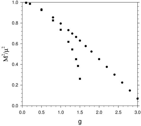
Figure 1: Mass-squared ratios $M^{2}/\mu^{2}$ versus dimensionless coupling strength $g$ for the LFCC approximation (squares) and the Fock-space truncation (circles).

To summarize, we have shown an application of the LFCC method to a model theory that requires numerical techniques. Also, suitable techniques have been developed, based on expansions in fully symmetric polynomials SymPoly . The results show important improvements over a Fock-space truncation approach. This provides a foundation for future work of greater complexity.

Such additional work could include investigation of convergence with respect to the terms in the truncated $T$ operator and analysis of symmetry breaking, for both positive and negative $\mu^{2}$. One approach to a study of symmetry breaking would be to consider the even eigenstates and search for degeneracy of the even and odd ground states. At least one additional term in the $T$ operator would be required, and the even valence state would have two constituents. A more complete analysis would include zero modes, for which some preliminary work has already been done LFCCzeromodes .

References

• (1) For reviews of light-cone quantization, see Burkardt M (2002) Light front quantization. Adv. Nucl. Phys. 23: 1-74; Brodsky SJ, Pauli H-C, Pinsky SS (1998) Quantum chromodynamics and other field theories on the light cone. Phys. Rep. 301: 299-486
• (2) Chabysheva SS, Hiller, JR (2012) A light-front coupled-cluster method for the nonperturbative solution of quantum field theories. Phys. Lett. B 711: 417-422
• (3) Elliott B, Chabysheva SS, Hiller JR (2014) Application of the light-front coupled-cluster method to $\phi^{4}$ theory in two dimensions. Phys. Rev. D 90: 056003
• (4) Dirac PAM (1949) Forms of relativistic dynamics. Rev. Mod. Phys. 21: 392-399
• (5) Perry RJ, Harindranath A, Wilson KG (1990) Light front Tamm–Dancoff field theory. Phys. Rev. Lett. 65: 2959-2962; Perry RJ, Harindranath, A (1991) Renormalization in the light front Tamm-Dancoff approach to field theory. Phys. Rev. D 43: 4051-4073
• (6) Hiller JR, Brodsky SJ (1998) Nonperturbative renormalization and the electron’s anomalous moment in large-$\alpha$ QED. Phys. Rev. D 59: 016006
• (7) Karmanov VA, Mathiot J-F, Smirnov AV (2008) Systematic renormalization scheme in light-front dynamics with Fock space truncation. Phys. Rev. D 77: 085028; Karmanov VA, Mathiot J-F, Smirnov AV (2010) Nonperturbative calculation of the anomalous magnetic moment in the Yukawa model within truncated Fock space. Phys. Rev. D 82: 056010
• (8) Chabysheva SS, Hiller JR (2010) On the nonperturbative solution of Pauli–Villars regulated light-front QED: A comparison of the sector-dependent and standard parameterizations. Ann. Phys. 325: 2435-2450
• (9) Chabysheva SS, Elliott B, Hiller JR (2013) Symmetric multivariate polynomials as a basis for three-boson light-front wave functions. Phys. Rev. E 88: 063307
• (10) Chabysheva SS, Hiller JR (2014) Zero modes in the light-front coupled-cluster method. Ann. Phys. 340: 188-204