Bifurcation to Chaos in the complex Ginzburg-Landau equation with large third-order dispersion.

Abstract

We give an analytic proof of the existence of Shilnikov chaos in complex Ginzburg-Landau equation subject to a large third-order dispersion perturbation.

The goal of this paper is to show that chaotic behavior is possible in complex Ginzburg-Landau equation with additional large dispersion term. The equation is

$$\partial_{t}u=(1+i\gamma)\partial^{2}_{x}u+\beta u-(1+i\omega)u|u|^{2}+L\partial^{3}_{x}u,$$ (1)

where $u$ is a complex-values function, spatially periodic with period $2\pi$, i.e. we consider Eq. (1) on the interval $x\in(-\pi,\pi)$ with the periodic boundary condition $u(-\pi)=u(\pi)$. The dispersion term $Lu_{xxx}$ causes fast temporal oscillations in the solution, so the evolution is described by effective averaged equation (see Eq. (3)). This averaging is performed in Ref. Kostianko et al. [2014]; it was also shown there that the averaging in a presence of the second-order dispersion term $iLu_{xx}$ with large $L$ leads to a significant simplification of the dynamics (the averaged system acquires a gradient structure). In this letter we show that, surprisingly, introducing the dispersion term as in Eq. (1) does not make dynamics gradient, and chaos can emerge in the averaged system. As the result is of an ideological nature, we refrained of the use of numerical integration. Instead, we provide an analytic proof of the existence of chaos in the averaged system (assisted by Maple and Mathematica tools).

As $L$ is large, Eq. (1) can be viewed as a perturbation of the auxiliary linear dispersion equation

$$u_{t}=Lu_{xxx}.$$ (2)

By choosing the orthogonal basis ${\bf e}_{n}=e^{inx}$, $n\in Z$, the flow $\mathcal{H}_{L}(t)$ generated by Eq. (2) is given by

$$\mathcal{H}_{L}(t){\bf e}_{n}=e^{in^{3}Lt}{\bf e}_{n}.$$

These solutions are $2\pi/L$-periodic with respect to time, i.e. they correspond to fast oscillations.

In order to average these oscillations, one makes the following change of variable $u$ in Eq. (1):

$$u(t)=\mathcal{H}_{L}(t)w(t)$$

The equations for $w$ acquire explicit rapidly oscillating terms. Averaging them out is done by Kostianko et al. [2014]. The result is the following equation:

$$\partial_{t}w=(1+i\gamma)\partial^{2}_{x}w+\beta w-(1+i\omega)N(w),$$ (3)

with the operator $N$ given by

$$N(w)=\left(2w\sum_{n\in Z}|w_{n}|^{2}+\bar{w}\sum_{n\in Z}w_{n}w_{-n}-2w_{0}|w_{0}|^{2}\right){\bf e}_{0}-\sum_{n\neq 0}w_{n}(|w_{n}|^{2}+2|w_{-n}|^{2}){\bf e}_{n},$$

where we denote $w=\sum_{n\in Z}w_{n}{\bf e}_{n}$, and $\bar{w}$ is the complex conjugate of $w$.

This is an infinite-dimensional system. It is shown in Ref. Kostianko et al. [2014] that it is well-posed and has a global attractor in an appropriate Sobolev space. The study of its full dynamics can be difficult, however this system has finite-dimensional invariant manifolds. One of these manifolds is

$$w_{n}=0\qquad\mbox{for all}\qquad|n|\geq 2.$$

In restriction to this space, we have $w=y{\bf e}_{0}+v({\bf e}_{1}+{\bf e}_{-1})$. Then

$$N(w)=(4y|v|^{2}+y|y|^{2}+2\bar{y}v^{2}){\bf e}_{0}+(v(2|y|^{2}+3|v|^{2})+\bar{v}y^{2})({\bf e}_{1}+{\bf e}_{-1}),$$

and Eq. (3) becomes

$$\left\{\begin{array}[]{l}\dot{y}=\beta y-(1+i\omega)\left[y(|y|^{2}+4|v|^{2})+2\bar{y}v^{2}\right],\\ \dot{v}=(\beta-1-i\gamma)v-(1+i\omega)\left[v(2|y|^{2}+3|v|^{2})+\bar{v}y^{2}\right].\end{array}\right.$$

Let $y=\sqrt{r}e^{i\varphi}$, $v=\sqrt{\rho}e^{i\psi}$. We obtain

$$\frac{\dot{r}}{2\sqrt{r}}e^{i\varphi}+i\dot{\varphi}\sqrt{r}e^{i\varphi}=\beta\sqrt{r}e^{i\varphi}-(1+i\omega)\left[\sqrt{r}e^{i\varphi}(r+4\rho)+2\sqrt{r}e^{-i\varphi}\rho e^{2i\psi}\right],$$

which gives

$$\dot{r}=2r\left[\beta-r-4\rho-2\rho(\cos\eta-\omega\sin\eta)\right],$$

$$\dot{\varphi}=-\omega(r+4\rho)-2(\sin\eta+\omega\cos\eta)\rho,$$

where $\eta=2(\psi-\varphi)$. Similarly,

$$\frac{\dot{\rho}}{2\sqrt{\rho}}e^{i\psi}+i\dot{\psi}\sqrt{\rho}e^{i\psi}=(\beta-1-i\gamma)\sqrt{\rho}e^{i\psi}-(1+i\omega)\left[\sqrt{\rho}e^{i\psi}(2r+3\rho)+\sqrt{\rho}e^{-i\psi}re^{2i\varphi}\right],$$

so

$$\dot{\rho}=2\rho\left[\beta-1-2r-3\rho-(\cos\eta+\omega\sin\eta)r\right],$$

$$\dot{\psi}=-\gamma-\omega(2r+3\rho)+(\sin\eta-\omega\cos\eta)r.$$

Finally (by scaling time to $2$), we obtain the following three-dimensional system:

$$\left\{\begin{array}[]{l}\dot{r}=r\left[\beta-r-4\rho-2\rho(\cos\eta-\omega\sin\eta)\right],\\ \dot{\rho}=\rho\left[\beta-1-2r-3\rho-(\cos\eta+\omega\sin\eta)r\right],\\ \dot{\eta}=-\gamma+\omega(\rho-r)+(\sin\eta-\omega\cos\eta)r+2(\sin\eta+\omega\cos\eta)\rho.\end{array}\right.$$ (4)

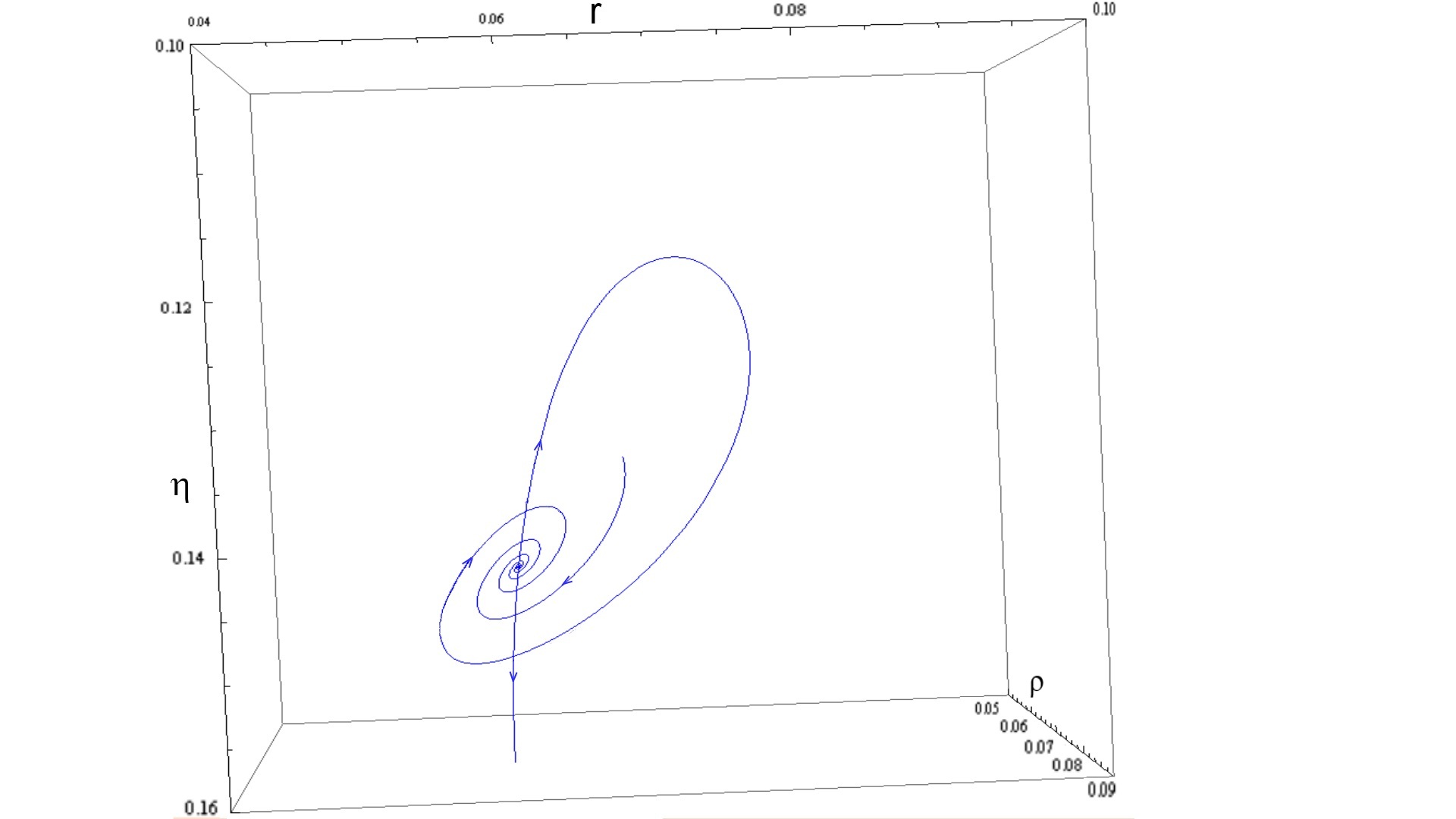
Figure 1: Homoclinic loop to the saddle-focus in system (4). The equilibrium is at $r=0.06$, $\rho=0.07221$, $\eta=0.143345$, which corresponds to $\omega\approx-30.965$, $\beta\approx 1.1306$, $\gamma\approx-2.9361$ (see Eqs. (5),(6)).

The computations that follow show that system (4) has a region of parameter values $(\beta,\gamma,\omega)$ which correspond to chaotic behavior. We prove this by showing that at a certain parameter value the system has Shilnikov saddle-focus homocinic loop Shilnikov [1965, 1970] (see also Ref. Afraimovich et al. [2014]). Doing this numerically would be an easy exercise – e.g. see in Fig. 1 a homoclinic loop we found in this system. However, we want to prove its existence analytically. To this aim, we employ the idea of Arneodo et al. [1985a, b] who showed that bifurcations of an equilibrium state with triple zero eigenvalue can lead to the birth of the Shlnikov loop. Fully analytic proof of this can be obtained using the result by Ibanez & Rodriguez [2005]; we also mention that this method was used for an analytic proof of (space-time) chaos in Ginzburg-Landau type equations by Turaev & Zelik [2010].

Thus, in the rest of the paper we are showing that system (4) has values of parameters which correspond to the equilibrium state that has all three eigenvalues zero and satisfies the conditions of Arneodo-Coullet-Spiegel-Tresser-Ibanez-Rodriguez theorem. It is easy to see that at non-zero $r$ and $\rho$, the equilibria are given by

$$\begin{array}[]{l}\beta=r+4\rho+2\rho(\cos\eta-\omega\sin\eta),\\ \beta=1+2r+3\rho+(\cos\eta+\omega\sin\eta)r,\\ \gamma=\omega(\rho-r)+(\sin\eta-\omega\cos\eta)r+2(\sin\eta+\omega\cos\eta)\rho.\end{array}$$ (5)

Thus, any $(r,\rho,\eta)$ can be an equilibrium for an appropriate choice of $\beta$ and $\gamma$, provided

$$\rho(1+2(\cos\eta-\omega\sin\eta))-r(1+(\cos\eta+\omega\sin\eta))=1.$$ (6)

The linearization matrix at the non-zero equilibrium is

$$A=\left(\begin{array}[]{ccc}-r&-2r(2+\cos\eta-\omega\sin\eta)&2r\rho(\sin\eta+\omega\cos\eta)\\ -\rho(2+\cos\eta+\omega\sin\eta)&-3\rho&r\rho(\sin\eta-\omega\cos\eta)\\ -\omega+\sin\eta-\omega\cos\eta&\omega+2(\sin\eta+\omega\cos\eta)&(\cos\eta+\omega\sin\eta)r+2(\cos\eta-\omega\sin\eta)\rho\end{array}\right).$$ (7)

We now look for the values of $r,\rho,\eta$ that correspond to a triple zero eigenvalue of $A$. This happens when the trace, determinant, and the sum $\sigma A$ of the three main second-order minors of $A$ are simultaneously zero.

Condition $trA=0$ reads as

$$r(1-\cos\eta-\omega\sin\eta)+\rho(3-2\cos\eta+2\omega\sin\eta)=0.$$ (8)

Note that if $\sin\eta=0$, then $trA$ cannot vanish at positive $r$ and $\rho$, so we further assume $\sin\eta\neq 0$.

The determinant of matrix $A$ vanishes when

$$\rho J_{1}+rJ_{2}=0$$

where

$$J_{1}=\left|\begin{array}[]{ccc}-1&-2(2+\cos\eta-\omega\sin\eta)&2(\sin\eta+\omega\cos\eta)\\ -(2+\cos\eta+\omega\sin\eta)&-3&0\\ -\omega+\sin\eta-\omega\cos\eta&\omega+2(\sin\eta+\omega\cos\eta)&2(\cos\eta-\omega\sin\eta)\end{array}\right|,$$

and

$$J_{2}=\left|\begin{array}[]{ccc}-1&-2(2+\cos\eta-\omega\sin\eta)&0\\ -(2+\cos\eta+\omega\sin\eta)&-3&\sin\eta-\omega\cos\eta\\ -\omega+\sin\eta-\omega\cos\eta&\omega+2(\sin\eta+\omega\cos\eta)&\cos\eta+\omega\sin\eta\end{array}\right|.$$

We have

$$J_{1}=-2(2+\cos\eta+\omega\sin\eta)\left|\begin{array}[]{cc}4+2(\cos\eta-\omega\sin\eta)&\sin\eta+\omega\cos\eta\\ -\omega-2(\sin\eta+\omega\cos\eta)&\cos\eta-\omega\sin\eta\end{array}\right|-$$

$$\qquad\qquad-6\left|\begin{array}[]{cc}-1&\sin\eta+\omega\cos\eta\\ -\omega+\sin\eta-\omega\cos\eta&\cos\eta-\omega\sin\eta\end{array}\right|=$$

$$=-(4+2\cos\eta+2\omega\sin\eta)\left[(4+\omega^{2})\cos\eta-3\omega\sin\eta+2(1+\omega^{2})\right]-$$

$$\qquad\qquad-6\left[(\omega^{2}-1)\cos\eta+2\omega\sin\eta-\sin^{2}\eta+\omega^{2}\cos\eta\right]=$$

$$=-2(1+\omega^{2})(1+7\cos\eta+2\omega\sin\eta+7\cos^{2}\eta+\omega\sin\eta\cos\eta),$$

and

$$J_{2}=-\left|\begin{array}[]{cc}-3&\sin\eta-\omega\cos\eta\\ \omega+2(\sin\eta+\omega\cos\eta)&\cos\eta+\omega\sin\eta\end{array}\right|-$$

$$\qquad\qquad-2(2+\cos\eta-\omega\sin\eta)\left|\begin{array}[]{cc}2+\cos\eta+\omega\sin\eta&\sin\eta-\omega\cos\eta\\ \omega-(\sin\eta-\omega\cos\eta)&\cos\eta+\omega\sin\eta\end{array}\right|=$$

$$=-\left[(\omega^{2}-3)\cos\eta-4\omega\sin\eta-2\sin^{2}\eta+2\omega^{2}\cos^{2}\eta\right]-$$

$$\qquad\qquad-(4+2\cos\eta-2\omega\sin\eta)\left[(2+\omega^{2})\cos\eta+\omega\sin\eta+1+\omega^{2}\right]=$$

$$=-(1+\omega^{2})(2+7\cos\eta-2\omega\sin\eta+6\cos^{2}\eta-2\omega\sin\eta\cos\eta).$$

Thus the condition $\det A=0$ is written as

$$\!\!\!\!\!\!\!\!\!\!\!\!2\rho(1+7\cos\eta+2\omega\sin\eta+7\cos^{2}\eta+\omega\sin\eta\cos\eta)+r(2+7\cos\eta-2\omega\sin\eta+6\cos^{2}\eta-2\omega\sin\eta\cos\eta)=0.$$ (9)

Under condition $trA=0$, matrix $A$ can be rewritten as

$$\left(\begin{array}[]{ccc}-r&-2r(2+\cos\eta-\omega\sin\eta)&2r\rho(\sin\eta+\omega\cos\eta)\\ -\rho(2+\cos\eta+\omega\sin\eta)&-3\rho&r\rho(\sin\eta-\omega\cos\eta)\\ -\omega+\sin\eta-\omega\cos\eta&\omega+2(\sin\eta+\omega\cos\eta)&r+3\rho\end{array}\right).$$

Its main second-order minors are

$$\left|\begin{array}[]{cc}-r&-2r(2+\cos\eta-\omega\sin\eta)\\ -\rho(2+\cos\eta+\omega\sin\eta)&-3\rho\end{array}\right|=r\rho(2\omega^{2}\sin^{2}\eta-5-8\cos\eta-2\cos^{2}\eta),$$

$$\left|\begin{array}[]{cc}-r&2r\rho(\sin\eta+\omega\cos\eta)\\ -\omega+\sin\eta-\omega\cos\eta&r+3\rho\end{array}\right|=-r(r+3\rho)-2r\rho(\sin^{2}\eta-\omega^{2}\cos^{2}\eta-\omega\sin\eta-\omega^{2}\cos\eta),$$

and

$$\left|\begin{array}[]{cc}-3\rho&r\rho(\sin\eta-\omega\cos\eta)\\ \omega+2(\sin\eta+\omega\cos\eta)&r+3\rho\end{array}\right|=-3\rho(r+3\rho)-r\rho(2\sin^{2}\eta-2\omega^{2}\cos^{2}\eta+\omega\sin\eta-\omega^{2}\cos\eta).$$

Thus, the sum $\sigma A$ of these minors vanishes (under condition $trA=0$) when

$$(r+3\rho)^{2}+r\rho(9-2\omega^{2}+(8-3\omega^{2})\cos\eta-\omega\sin\eta-2(1+\omega^{2})\cos^{2}\eta)=0.$$ (10)

We are looking for values of $r,\rho,\eta,\omega$ which solve the system of Eqs. (6),(8),(9),(10). From Eq. (8) we find

$$\rho=r\frac{-1+\cos\eta+\omega\sin\eta}{3-2\cos\eta+2\omega\sin\eta}.$$ (11)

By plugging this into Eqs. (9) and (10), we obtain the following system of equations for $q=\omega\sin\eta$ and $z=\cos\eta$ (so $\omega^{2}=\frac{q^{2}}{1-z^{2}}$):

$$2(-1+z+q)(1+7z+7z^{2}+2q+qz)+(3-2z+2q)(2+7z+6z^{2}-2q-2qz)=0,$$

and

$$(z+5q)^{2}+(-1+z+q)(3-2z+2q)(9-2\frac{q^{2}}{1-z^{2}}+(8-3\frac{q^{2}}{1-z^{2}})z-q-2(1+\frac{q^{2}}{1-z^{2}})z^{2})=0.$$

This recasts as

$$2q^{2}z-q(32z^{2}+28z-4)-2z^{3}-4z^{2}-5z-4=0,$$ (12)

and

$$(1-z^{2})(z^{2}+10yz+25q^{2})+(2q^{2}+q-2z^{2}+5z-3)(9+8z-11z^{2}-8z^{3}+2z^{4}-q(1-z^{2})-(2+3z+2z^{2})q^{2})=0,$$

or

$$2(2z^{2}+3z+2)q^{4}+q^{3}(4+3z)-q^{2}(8z^{4}-20z^{3}-51z^{2}+15z+48)+$$

$$\qquad\qquad+q(z^{2}-1)(12+13z)+(z^{2}-1)(4z^{4}-26z^{3}+29z^{2}+21z-27)=0,$$

or

$$\!\!\!\!\!\!\!\!\!\!\!\!\!\!\!\!(2z^{2}(2z^{2}+3z+2)q^{2}+z(64z^{4}+152z^{3}+143z^{3}+48z-8)q+1020z^{6}+3362z^{5}+4365z^{4}+2482z^{3}+232z^{2}-200z+16)\times$$

$$\qquad\times(2q^{2}z-q(32z^{2}+28z-4)-2z^{3}-4z^{2}-5z-4)=$$

$$\qquad\qquad=(32768z^{8}+136704z^{7}+230976z^{6}+189904z^{5}+60933z^{4}-9076z^{3}-5864z^{2}+1216z-64)q+$$

$$\qquad\qquad\qquad+2048z^{9}+10752z^{8}+27328z^{7}+43408z^{6}+45553z^{5}+30356z^{4}+10374z^{3}-8z^{2}-720z+64.$$

By Eq. (12), this gives us

$$\!\!\!\!\!\!\!\!\!\!\!\!\!\!\!\!\omega\sin\eta=q=-\frac{2048z^{9}+10752z^{8}+27328z^{7}+43408z^{6}+45553z^{5}+30356z^{4}+10374z^{3}-8z^{2}-720z+64}{32768z^{8}+136704z^{7}+230976z^{6}+189904z^{5}+60933z^{4}-9076z^{3}-5864z^{2}+1216z-64}.$$ (13)

By inserting this expression into Eq. (12) we obtain the following equation for $z$:

$$2(2048z^{9}+10752z^{8}+27328z^{7}+43408z^{6}+45553z^{5}+30356z^{4}+10374z^{3}-8z^{2}-720z+64)^{2}z+$$

$$+(2048z^{9}+10752z^{8}+27328z^{7}+43408z^{6}+45553z^{5}+30356z^{4}+10374z^{3}-8z^{2}-720z+64)\times$$

$$\qquad\qquad\qquad\times(32768z^{8}+136704z^{7}+230976z^{6}+189904z^{5}+60933z^{4}-9076z^{3}-5864z^{2}+1216z-64)\times$$

$$\qquad\qquad\qquad\qquad\qquad\times(32z^{2}+28z-4)-$$

$$-(2z^{3}+4z^{2}+5z+4)(32768z^{8}+136704z^{7}+230976z^{6}+189904z^{5}+60933z^{4}-9076z^{3}-5864z^{2}+1216z-64)^{2}=0,$$

or

$$P(z)=-512-1536z+123584z^{2}-294656z^{3}-2669168z^{4}-1014068z^{5}+16713471z^{6}+38944576z^{7}+$$

$$\quad+29896640z^{8}-11432448z^{9}-38759936z^{10}-28958720z^{11}-8060928z^{12}+524288z^{13}+524288z^{14}=0.$$

This polynomial has the following roots in the interval $[-1,1]$:

$$z\approx-.8468602601,-.8453251846,-.05672395050,.09599192317,.1369140710,.2980830761,.982719862$$

The root $z=\cos\eta=z_{0}\approx.136914071$ corresponds to

$$\eta=\eta_{0}\approx 1.433450854.$$

By Eq. (13) one finds

$$\omega=\omega_{0}\approx-3.487162,$$

and, by Eqs. (6),(11),

$$r=r_{0}\approx 0.092903423,\quad\rho=\rho_{0}\approx 0.09590066.$$

One may check that the other roots of $P(z)$ do not produce positive values of $r$ and $\rho$. The corresponding values of $\beta=\beta_{0}$ and $\gamma=\gamma_{0}$ are found from Eq. (5):

$$\beta_{0}\approx 1.16531,\gamma_{0}\approx 0.224354$$

Note that $P^{\prime}(z_{0})\approx-6633\neq 0$, therefore any small perturbation of the system of Eqs. (8),(9),(10),(6) will have a solution $(r,\rho,\omega,\eta)$ close to $(r_{0},\rho_{0},\eta_{0})$. Thus, for any given small values $\mu,\nu,\lambda$, we can always find values of parameters $(\beta,\gamma,\omega)$ close to $(\beta_{0},\gamma_{0},\omega_{0})$ which would correspond to the existence of an equilibrium state close to $(r_{0},\rho_{0},\eta_{0})$ such that the linearization matrix $A$ at this equilibrium will have $trA=\mu$, $\sigma A=\nu$ and $detA=\lambda$.

Consider system (4) at $(\beta,\gamma,\omega)=(\beta_{0},\gamma_{0},\omega_{0})$. We put the coordinate origin to the equilibrium, i.e. we denote $x_{1}=r-r_{0},x_{2}=\rho-\rho_{0},x_{3}=\eta-\eta_{0}$. The system takes the form

$$\dot{x}=Ax+F(x)+O(\|x\|^{3})$$

where $F(x)$ contains only quadratic terms; recall that the matrix $A$ has three zero eigenvalues, so $A^{3}=0$. We take the vectors $A^{2}e$, $Ae$ and $e=\left(\begin{array}[]{c}0\\ 1\\ 0\end{array}\right)$ as the coordinate basis. In other words, we make a coordinate transformation $x=QX$, where $Q=(A^{2}e,Ae,e)$. One needs to check that $det(Q)\neq 0$; then the system takes the form

$$\frac{d}{dt}\left(\begin{array}[]{c}X_{1}\\ X_{2}\\ X_{3}\end{array}\right)=\left(\begin{array}[]{c}X_{2}\\ X_{3}\\ 0\end{array}\right)+Q^{-1}F(QX)+O(\|X\|^{3}).$$

Moreover, when we add any small perturbation to this system we can always choose coordinates so that $\dot{X}_{1}=X_{2}$ and $\dot{X}_{2}=X_{3}$. Thus, if a perturbation of the $C^{2}$-size $\delta$ is added so that the equilibrium state does not disappear, the system takes the form

$$\frac{d}{dt}\left(\begin{array}[]{c}X_{1}\\ X_{2}\\ X_{3}\end{array}\right)=\left(\begin{array}[]{c}X_{2}\\ X_{3}\\ \lambda X_{1}-\nu X_{2}+\mu X_{3}\end{array}\right)+Q^{-1}F(QX)+O(\|X\|^{3}+\delta\|X\|^{2}).$$ (14)

As we just mentioned, the coefficients $\mu=trA$, $\nu=\sigma A$ and $\lambda=detA$ can acquire arbitrary small values when the parameters $\beta,\gamma,\omega$ are changed appropriately. It has been shown in Refs. Arneodo et al. [1985a]; Ibanez & Rodriguez [2005] that systems of form (14) have chaotic dynamics (the Shilnikov saddle-focus loop) at some values of $\mu,\nu,\lambda$ (which can be chosen arbitrarily small), provided the the coefficient $a$ of $X_{1}^{2}$ in the equation for $\dot{X}_{3}$ is not zero.

Thus, to prove the existence of chaotic behavior in system (4), it remains to compute $detQ$ and $a$. By plugging the values of $r_{0},\rho_{0},\eta_{0},\omega_{0}$ into Eq. (7), we find

$$A\approx\left(\begin{array}[]{ccc}-0.09290342&-1.0388902&0.009143666\\ 0.1263404&-0.287702&0.01307936\\ 4.955187&-2.460879&0.3806054\end{array}\right),$$

$$A^{2}\approx\left(\begin{array}[]{ccc}-0.07731418&0.3729058&-0.01095737\\ 0.01672483&-0.080668085&0.0023703315\\ 1.1147085&-5.376519&0.1579823\end{array}\right).$$

Thus, the matrix $Q=(A^{2}e,Ae,e)$ is given by

$$Q\approx\left(\begin{array}[]{ccc}0.3729058&-1.0388902&0\\ -0.080668085&-0.287702&1\\ -5.376519&-2.460879&0\end{array}\right).$$

We have $detQ\approx 6.503289\neq 0$, so the system can indeed be brought to form (14).

It remains to find the coefficient $a$ of $X_{1}^{2}$ in the equation for $\dot{X}_{3}$ in Eq. (14)). It equals to the product of the third row of the matrix $Q^{-1}$ to $f(A^{2}e)$. The third row of $Q^{-1}$ is orthogonal to the first and second columns of $Q$, i.e. to the vectors $A^{2}e$ and $Ae$. Any row of the matrix $A^{2}$ satisfies this property (recall that $A^{3}=0$). Therefore, in order to check that $a\neq 0$, it is enough to check that the product $f(A^{2}e)$ to the third row of $A^{2}$ is non-zero. Since $f$ is the quadratic part of the Taylor expansion of the right-hand side of system (4) at the point $(r_{0},\rho_{0},eta_{0})$, we need to compute the coefficient of $\varepsilon^{2}$ in the expansion in powers of $\varepsilon$ for $p_{1}\dot{r}+p_{2}\dot{\rho}+p_{3}\dot{\eta}$ evaluated at $(r,\rho,\eta)=(r_{0}+q_{1}\varepsilon,\rho_{0}+q_{2}\varepsilon,\eta_{0}+q_{3}\varepsilon)$, where $(p_{1},p_{2},p_{3})$ is the third row of $A^{2}$ and $(q_{1},q_{2},q_{3})^{\top}=A^{2}e$ is the second column of $A^{2}$; recall that

$$p_{1}\approx 1.1147085,\qquad p_{2}\approx-5.376519,\qquad p_{3}\approx 0.1579823,$$

$$q_{1}\approx 0.3729058,\qquad q_{2}\approx-0.080668085,\qquad q_{3}\approx-5.376519.$$

We have

$$p_{1}\dot{r}+p_{2}\dot{\rho}+p_{3}\dot{\eta}=-p_{1}r^{2}-3p_{2}\rho^{2}-r\rho(4p_{1}+2p_{1}(\cos\eta-\omega\sin\eta)+p_{2}(2+\cos\eta+\omega\sin\eta))+$$

$$+p_{3}(\sin\eta-\omega\cos\eta)r+2p_{3}(\sin\eta+\omega\cos\eta)\rho+\mbox{ linear terms}.$$

By plugging $(r,\rho,\eta)=(r_{0}+q_{1}\varepsilon,\rho_{0}+q_{2}\varepsilon,\eta_{0}+q_{3}\varepsilon)$ in the right-hand side, we find that the coefficient of $\varepsilon^{2}$ equals to

$$-p_{1}q_{1}^{2}-3p_{2}q_{2}^{2}-q_{1}q_{2}(4p_{1}+2p_{2}+(2p_{1}+p_{2})\cos\eta_{0}+(p_{2}-2p_{1})\omega_{0}\sin\eta_{0})+$$

$$+(q_{1}\rho_{0}+q_{2}r_{0})q_{3}((2p_{1}+p_{2})\sin\eta_{0}+(2p_{1}-p_{2})\omega_{0}\cos\eta_{0})+\frac{1}{2}r_{0}\rho_{0}q_{3}^{2}((2p_{1}+p_{2})\cos\eta_{0}+(p_{2}-2p_{1})\omega_{0}\sin\eta_{0})-$$

$$-\frac{1}{2}p_{3}q_{3}^{2}(\sin\eta_{0}-\omega_{0}\cos\eta_{0})r_{0}+p_{3}q_{3}q_{1}(\cos\eta_{0}+\omega_{0}\sin\eta_{0})-p_{3}q_{3}^{2}(\sin\eta_{0}+\omega_{0}\cos\eta_{0})\rho_{0}+$$

$$+2p_{3}q_{3}q_{2}(\cos\eta_{0}-\omega_{0}\sin\eta_{0})\approx 5.898,$$

i.e. it is non-zero. This finishes the proof of the existence of chaotic dynamics in system (4).

References

Afraimovich et al. [2014] Afraimovich, V.S., Gonchenko, S.V., Lerman, L., Shilnikov, A., Turaev, D. [2014]
“Scientific heritage of L.P.Shilnikov,” Regul. Chaotic Dyn.19, 435–460.
Arneodo et al. [1985a] Arneodo, A., Coullet, P.H., Spiegel, E.A., & Tresser, C., [1985] “Asymptotic Chaos,” em Physica D 14, 327–347.
Arneodo et al. [1985b] Arneodo, A., Coullet, P.H., & Spiegel, E.A. [1985] “The dynamics of triple convection,”
Geophys. Astrophys. Fluid Dyn.31, 1–48.
Ibanez & Rodriguez [2005] Ibanez, S. & Rodriguez, J. A. [2005] “Shilnikov configurations in any generic unfolding of the nilpotent
singularity of codimension three on ,” J. Differential Equations208, 147–175.
Kostianko et al. [2014] Kostianko, A., Titi, E., & Zelik, S.
[2014] “Large dispersion, averaging, and attractors: three 1D paradigms,” preprint.
Shilnikov [1965] Shilnikov, L. P. [1965] “A case of the existence of a countable number of periodic motions,” Soviet Math.
Dokl.6, 163–166.
Shilnikov [1970] Shilnikov, L. P. [1970] “A contribution to the problem of the structure of an extended neighbourhood
of a rough equilibrium state of saddle-focus type,” Math. USSR-Sb.10, 91–102.
Turaev & Zelik [2010] Turaev, D. & Zelik, S. [2010] “Analytical proof of space-time chaos in Ginzburg Landau Equations,”
Discrete Contin. Dyn. Syst.28, 1713–1751.