On the integration of stochastic rigid body with geometric numerical schemes

Abstract

In the present paper we investigate the performance of explicit splitting schemes and related techniques applied to a rigid body model subject to a stochastic torque and random perturbations in the inertia tensor. Results are discussed and compared with traditional solvers for such model.

1 Introduction

Stochastic differential equations (SDEs) are used in many fields, such as stock market, financial mathematics, stochastic controls, biological science, chemical reactive kinetics and hydrology, as described in [15], [18]. Thus, it is of importance to study the solution of SDEs. However, finding the analytic solutions is often very difficult or impossible. Numerical methods, on the other hand, help to find approximate solutions of SDEs quite fast, and thus, development of such methods looks promising. However, it is of importance to study the solution of SDEs obtained numerically, because of results obtained by different methods may deviate significantly in terms of accuracy and computational resources required.

Many of the physical systems could be refined in terms of generalized stochastic rigid body model. For example, this model might be rigid body subject to small perturbation force randomly dependent on time, or the body with randomly perturbed inertia. Examples of such an approach could be found in polymer simulations when the polymer chain is divided into several interacting monomers treated as rigid bodies during the modelling. The stochastic torques arise when the polymer is immersed in a solvent: the kinematics of each of the bodies in the model is influenced by stochastic loads raised from thermal fluctuations [16].

Another example is considered in the work by Arnold et al. [2] where authors concentrate on a ship partly immersed in water. The authors propose a stochastic model which includes an impact of severe weather conditions such as seaway and wind on a roll motion of the ship.

Another example arises in the field of animation [17], where a light body flying through air is simulated by solving generalized Kirchhoff equations. The challenge is to determine resulted forces and torques due to the turbulence generated at the body surface (vortical loads). In order to do that effectively the authors suggest a coupled approach: solve the free rigid body equations with no vortical loads and then generalized Langevin equations used to represent the characteristics of the surrounding flow.

Each of the above examples is treated with specifically tailored numerical schemes.

In this work we focus on the evolution of the angular momentum of a rigid body subject to a stochastic torque. This simple test case is used here for testing our numerical schemes. We also study a rigid body model with randomly perturbed inertia tensor. This is of interest in the case of multibody system dynamics with uncertain rigid bodies as studied in [3].

We consider two techniques: a splitting method and a method based on the variation of constants formula. These are well known techniques for deterministic problems which we here want to test in a stochastic context. We believe these techniques have some potential also for more complex problems [3], [17], [2] then the ones considered here.

We start with the formulation of the mathematical model followed by the description of the numerical schemes. Then we apply a variety of numerical schemes and investigate them in terms of weak errors. We compare the methods in terms of CPU time and relative cost. Further we investigate the geometrical properties of the numerical methods applied to the model with randomly perturbed inertia.

2 Rigid body under random perturbation

2.1 Mathematical model

We study the following stochastic differential equation with one-dimensional Brownian motion

$$d\boldsymbol{m}=(\boldsymbol{m}\times T^{-1}\boldsymbol{m})dt+a\,\boldsymbol{m}\,dW_{t},\qquad\boldsymbol{m}(0)=\boldsymbol{m}_{0}$$ (1)

where $\boldsymbol{m}\in\mathbb{R}^{3}$ is the angular momentum of the body, $T\in\mathbb{R}^{3\times 3}$ is a diagonal inertia matrix, $\boldsymbol{\omega}=T^{-1}\boldsymbol{m}\in\mathbb{R}^{3}$ is angular velocity, $W_{t}$ is a standard Brownian motion, $a$ is a parameter (noise). We assume that the three moments of inertia are pairwise distinct and we order them in ascending order.

2.2 Numerical methods

2.2.1 Splitting scheme

Since (1) is a sum of two exactly solvable terms and splitting it into deterministic and stochastic parts gives us exact solution

$$S_{1}\,:\qquad d\boldsymbol{m}=(\boldsymbol{m}\times T^{-1}\boldsymbol{m})dt$$ (2)

$$S_{2}\,:\qquad d\boldsymbol{m}=a\,\boldsymbol{m}\,dW_{t}$$ (3)

then we compose the flows of systems (2) and (3) into the first order splitting scheme

$$(\boldsymbol{m},q)^{(j+1)}=\phi_{h}^{[S_{2}]}\circ\phi_{h}^{[S_{1}]}\,((\boldsymbol{m},q)^{(j)}).$$ (4)

The first equations (2) are a free rigid body motion equations and could be integrated exactly. An explicit solution can be obtained by using Jacobi elliptic functions and has been implemented to machine accuracy following the techniques presented in [4]. The solution of the second set of equations (3) is

$$\boldsymbol{m}(t)=\exp\left(a\,W(t)-\frac{1}{2}\,a^{2}t\right)\boldsymbol{m}_{0}$$ (5)

where $W(t)$ is independent random variable of the form $\sqrt{t}N(0,1)$.

2.2.2 The Variation of Constants formula

We recall the variation of constants formula. Let us consider the following system of differential equations

$$\dot{\boldsymbol{z}} =f(\boldsymbol{z})+g(\boldsymbol{z}), \boldsymbol{z}(0) =y_{0},$$ (6)

$$\dot{\boldsymbol{y}} =f(\boldsymbol{y}), \boldsymbol{y}(0) =y_{0}$$

and suppose that $\frac{\partial f}{\partial\boldsymbol{y}}$ exists and is continuous. Then the solution is given by the non-linear variation of constants formula [12] (p.96, Chapter 1).

$$\boldsymbol{z}(t)=\boldsymbol{y}(t)+\int_{0}^{t}\Phi(t,\,s,\,\boldsymbol{z}(s))\cdot g(\boldsymbol{z}(s))ds,$$ (7)

with $\Phi$ is the solution of the equation

$$\begin{array}[]{lcl}\Phi^{\prime}=\frac{\partial f}{\partial\boldsymbol{y}}(\boldsymbol{y})\cdot\Phi,\\ \Phi(0)=I{{}_{3\times 3}}\\ \end{array}$$ (8)

solved together with $\dot{\boldsymbol{y}}=f(\boldsymbol{y})$. For our problem in order to integrate (1) with the variation of constants formulae we set

$$\dot{\boldsymbol{y}}=f(\boldsymbol{y})=\boldsymbol{y}\times T^{-1}\boldsymbol{y},$$ (9)

and

$$g\,dt=a\,\boldsymbol{z}dW_{t}.$$ (10)

Let us denote with

$$A(t,\boldsymbol{y})=\frac{\partial f}{\partial\boldsymbol{y}}(\boldsymbol{y})$$

then we obtain

$$A(t,\boldsymbol{z})=\left(\begin{array}[]{ccc}0&\boldsymbol{z}(3)(\frac{T_{2}-T_{3}}{T_{2}T_{3}})&\boldsymbol{z}(2)(\frac{T_{2}-T_{3}}{T_{2}T_{3}})\\[6.0pt] \boldsymbol{z}(3)(\frac{T_{3}-T_{1}}{T_{1}T_{3}})&0&\boldsymbol{z}(1)(\frac{T_{3}-T_{1}}{T_{1}T_{3}})\\[6.0pt] \boldsymbol{z}(2)(\frac{T_{1}-T_{2}}{T_{2}T_{1}})&\boldsymbol{z}(1)(\frac{T_{1}-T_{2}}{T_{2}T_{1}})&0\end{array}\right).$$

Then we use (7) to construct our numerical approximation $\boldsymbol{z}_{n+1}=\boldsymbol{y}_{n+1}+a\,dW_{n}\,\Phi_{n+1}\boldsymbol{z}_{n}$, where $\boldsymbol{y}_{n+1}$ is a solution of (9), $\Phi_{n+1}$ is a solution of (8), $dW_{n}$ is a Brownian increment. Equation (9) is a free rigid body problem and we solve it exactly with Jacobi elliptic functions [4], obtaining $\boldsymbol{y}_{1}=\boldsymbol{y}(t_{1}),\,\dots,\,\boldsymbol{y}_{n}=\boldsymbol{y}(t_{n})$. We integrate (8) with a Magnus method of order two [11] and get

$$\Phi_{n+1}=\exp(hA(t_{n}+h/2,{\boldsymbol{z}_{n+1/2}}))\Phi_{n},$$ (11)

where

$$\boldsymbol{z}_{n+1/2}=\boldsymbol{y}_{n+1/2}+a\,dW_{n}\,\Phi_{n+1/2}\boldsymbol{z}_{n},\quad\Phi_{n+1/2}=\exp(hA(t_{n}+h/2,\boldsymbol{y}_{n+1/2}))\Phi_{n}.$$

3 Random perturbation of inertia tensor

Consider a free rigid body model subject to white noise in inertia

$$\dot{\boldsymbol{m}}=\boldsymbol{m}\times T^{-1}\boldsymbol{m},\qquad\boldsymbol{m}(0)=\boldsymbol{m}_{0}$$ (12)

with $T=T_{d}+T_{s}$, $T_{d}$ is a deterministic inertia tensor, $T_{s}=\epsilon\,W$ with a small parameter $\epsilon$ and an arbitrary martingale

$$W=\left(\begin{array}[]{ccc}\xi_{11}&\xi_{12}&\xi_{13}\\ \xi_{21}&\xi_{22}&\xi_{23}\\ \xi_{31}&\xi_{32}&\xi_{33}\end{array}\right),\quad\xi_{ij}\in\mathbb{R}$$

We then need to calculate an inverse of the inertia matrix

$$(T_{d}+T_{s})^{-1}=T_{d}^{-1}(I{{}_{3\times 3}}+T_{s}T_{d}^{-1})^{-1}.$$

Assuming $\|T_{s}T_{d}^{-1}\|<1$ with $\|\bullet\|$ any matrix norm, we can apply Neumann series (for which convergence guaranteed) and we get

$$T_{d}^{-1}\sum_{k=0}^{\infty}(T_{s}T_{d}^{-1})^{k}=T_{d}^{-1}(I{{}_{3\times 3}}+\sum_{k=1}^{\infty}(T_{s}T_{d}^{-1})^{k})=T_{d}^{-1}+\sum_{k=1}^{\infty}(T_{s}T_{d}^{-1})^{k}.$$

Assume $\tilde{T_{d}}=T_{d}^{-1}$ and $\tilde{T_{s}}=\sum_{k=1}^{\infty}(T_{s}T_{d}^{-1})^{k},$ such that

$$\left\{\begin{array}[]{lcl}\dot{\boldsymbol{m}}&=&\boldsymbol{m}\times\tilde{T_{d}}\boldsymbol{m}+\boldsymbol{m}\times\tilde{T_{s}}\boldsymbol{m},\\ \dot{q}&=&\frac{1}{2}q\,\Omega\end{array}\right.$$ (13)

3.1 Numerical solution

In the case of random perturbation of inertia tensor we split (13) into stochastic and deterministic parts

$$S_{1}\,:\qquad\dot{\boldsymbol{m}}=\boldsymbol{m}\times\tilde{T_{d}}\boldsymbol{m}$$ (14)

and

$$S_{2}\,:\qquad\dot{\boldsymbol{m}}=\boldsymbol{m}\times\tilde{T_{s}}\boldsymbol{m}$$ (15)

We then combine the two flows into Lie-Trotter scheme.

We shall also use solution from (fully) implicit midpoint rule given by the general scheme in stochastic setting [13]

$$X_{n+1}=X_{n}+h\,f\left(\frac{X_{n}+X_{n+1}}{2}\right),$$ (16)

where $X_{n}$ is a numerical approximation of $\dot{X}=f(X)$.

4 Results and discussion

Firstly we show the weak convergence of the splitting method, the Euler-Maruyma (EM) and the Variation-of-Constants (VoC) methods applied to problem (1). Figure 1 shows the absolute error between mean values over sampled paths $|\mathbb{E}(\boldsymbol{m}(T))-\mathbb{E}(\boldsymbol{m}_{ref})|$ in the angular momentum versus time integration step. Initial values $\boldsymbol{m}_{0}$ = [0.4165;0.9072;0.0577], T= diag([0.9144;1.098;1.66]), $a=0.1$, integration time t = 1. The number of integration steps have been set ranging from $2^{1}$ up to $2^{9}$ and equally spaced in logarithmic scale. S = 1000 paths are sampled. For a reference solution we take the approximated one with step-size $2^{-8}$.

On Figure 2 one can see the weak convergence of splitting solver (4) applied to (14), (15) and the free rigid body (FRB) integrator [4]. We note the error in reference solution significantly depends on number of paths sampled, see Table 1.

Table 1: Absolute error in reference solution vs number of Brownian paths sampled

S	Error
100	0.0016
1000	4.38e-04
10000	6.38e-05
100000	7.71e-05

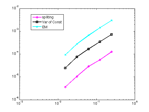
Figure 1: Error $|\mathbb{E}(\boldsymbol{m}(T))-\mathbb{E}(\boldsymbol{m}_{ref})|$ where $\boldsymbol{m}$ a solution of (1) with Lie-Trotter splitting the Euler-Maruyma and Variation of Constants.

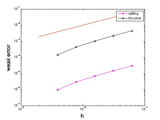
Figure 2: Error $|\mathbb{E}(\boldsymbol{m}(T))-\mathbb{E}(\boldsymbol{m}_{ref})|$ with $\boldsymbol{m}$ a solution of (12) with (4) (magenta) and FRB integrator (black). Reference red line has slope one.

From the above Figure 1 it is easy to see that the EM scheme, the splitting scheme and the VoC have the order one weak convergence, but the splitting scheme obtains better approximate solutions for the problem (1). The evaluation of CPU time used for the calculations have been performed directly in MATLAB® by measuring the time interval between the initiation of the algorithm and completion of the calculation. The performance of the algorithm is well represented by the plot of the weak error in $\boldsymbol{m}$ against the CPU time (Figure 3). The amount of calculations is proportional to the number of integration steps hence we expect the EM to be the fastest when no high accuracy is required.

The relative cost of the method can be computed as a ratio between given method cost and the minimal cost of method. The cost of Euler-Maruyma method is minimal compare to the Variation of Constants and splitting scheme. We see that the relative cost of the splitting scheme and variation of constants is decreasing for large step-sizes. This makes them attractive when large step-sizes are required in simulations.

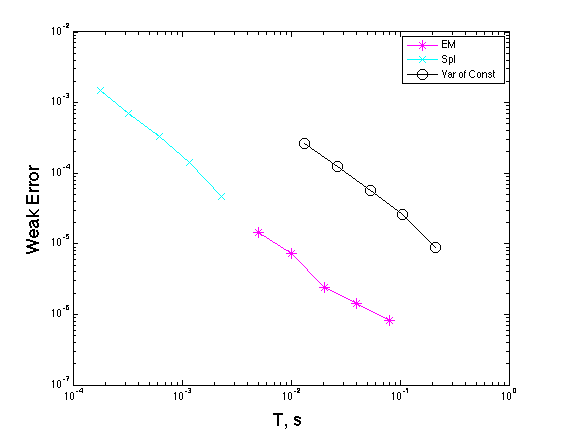
Figure 3: Average log of error versus cpu time (1000 Brownian paths).

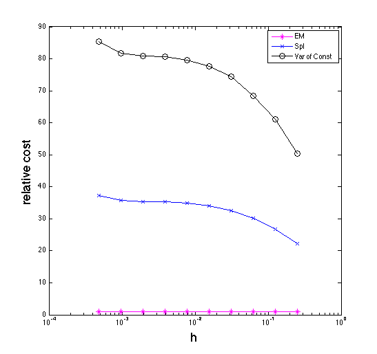
Figure 4: Relative cost (with respect to the cheapest method) versus step-size

We next consider a perturbed rigid body where the perturbation is given by a random torque. A similar problem has been considered in the deterministic case for example in [6]. The aim of the experiments is to see how the trajectories of the momentum are affected by the size of the noise. We see that the numerical trajectory maintains the same character of the free rigid body motion when the noise parameter $a$ is small enough see Figure 5. This behaviour is due to usage of free rigid solver based on Jacobi elliptic functions [6], [4], [5]. However when the noise term starts increasing the trajectory of variation of constants method does not look smooth anymore, see Figure 6.

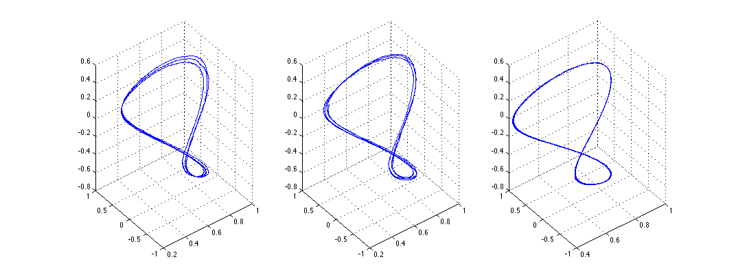
Figure 5: The vector $\boldsymbol{m}_{i}\approx\boldsymbol{m}(ih)$ for the perturbed rigid body motion over time T=10000 with h=0.1, noise parameter a=0.001. Left splitting method; middle EM method; right variation of constants

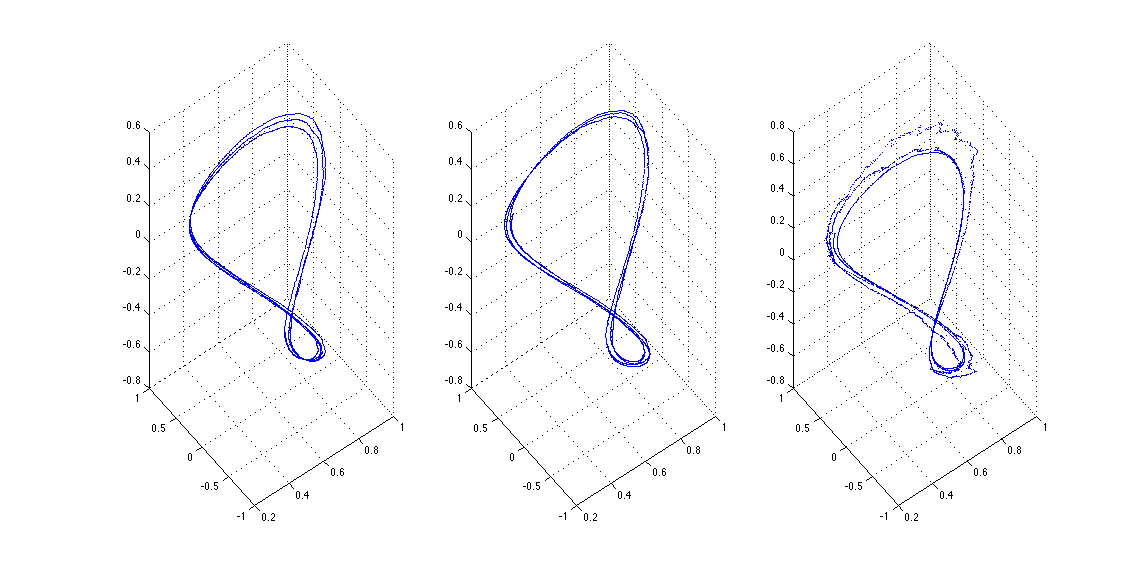
Figure 6: The vector $\boldsymbol{m}_{i}\approx\boldsymbol{m}(ih)$ for the perturbed rigid body motion over time T=10000 with h=0.1, noise parameter a=0.005. Left splitting method; middle EM method; right variation of constants

Another issue, that might be of interest is the preservation of angular momentum in models with random inertia. Also we look at energy of the model and see to which extent it preserved. We compare our results with the implicit midpoint rule and present them in Figure 7. We measure the energy as

$$H=\frac{1}{2}\omega^{T}\,T\,\omega,$$ (17)

with $\boldsymbol{\omega}=T^{-1}\boldsymbol{m}\in\mathbb{R}^{3}$, $T=T_{d}+T_{s}$. The energy error is averaged over 100 Brownian samples.

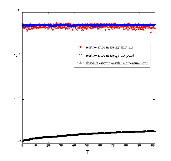
Figure 7: Energy error for the body with random inertia. Integration on the interval [0,100], h=0.25, using the splitting method and the midpoint rule.

5 Conclusion

In the current work we have performed numerical methods, which widely used for deterministic problems, to simple stochastic models. We see that methods work the same way as expected. We propose that these well know methods have a prospectiveness for more advanced stochastic models.

6 Acknowledgements

This research was supported by a Marie Curie International Research Staff Exchange Scheme Fellowship within the 7th European Community Framework Programme. The authors would like to acknowledge the support from the GeNuIn Applications project funded by the Research Council of Norway, and part of the work was carried out while the authors were visiting Massey University, Palmerston North, New Zealand and La Trobe University, Melbourne, Australia.

References

- [1] S. Blanes and P.C. Moan. Practical symplectic partitioned Runge-Kutta and Runge-Kutta-Nyström methods Journal of Computational and Applied Mathematics, 142:313–330, 2002.
- [2] L. Arnold, I. Chueshov, and G. Ochs. Random Dynamical Systems Methods in Ship Stability: A Case Study Journal of Physics A, 39:5463–5478, 2006.
- [3] A. Batou, C. Soize Multibody system dynamics with uncertain rigid bodies. Proceedings of the 8th International Conference on Structural Dynamics, EURODYN 2011, 2620–2625.
- [4] E. Celledoni, F. Fassó, N. Säfström and A. Zanna. The exact computation of the free rigid body motion and its use in splitting methods SIAM Journal on Scientific Computing, 30:4:2084–2112, 2008.
- [5] E. Celledoni and N. Säfström. Efficient time-symmetric simulation of torqued rigid bodies using Jacobi elliptic functions. Journal of Rhysics A, Vol. 39, pp. 5463–5478, 2006
- [6] E. Celledoni and A. Zanna. FRB-FORTRAN routines for the exact computation of free rigid body motions ACM ToMS, vol 37 nr. 2 (2010).
- [7] N.A. Chaturvedi, A.K. Sanyal and N.H. McClamroch Rigid-Body Attitude Control IEEE Control Systems Magazine, 31:3:30–51, 2011.
- [8] A. Dullweber, B. Leimkuhler, and R. McLachlan. Symplectic splitting methods for rigid body molecular dynamics. J. Chem. Phys, 107:5840–5851, 1997.
- [9] T.I. Fossen. Marine Control Systems. Marine Cybernetics, 2002.
- [10] M. Geradin and A. Cardona. Flexible Multibody Dynamics. Wiley and Sons Ltd., 2001.
- [11] E. Hairer, C. Lubich, and G. Wanner. Geometric numerical integration, volume 31 of Springer series in computational mathematics. Springer series in computational mathematics, volume 31. Springer, 2002.
- [12] E. Hairer, S.P. Nørsett and G. Wanner. Solving Ordinary Differential equations. Nonstiff Problems. Springer series in computational mathematics 8. Springer, Berlin, 2002.
- [13] G.N. Milstein, Yu.M. Repin, and M.V. Tretyakov. Numerical Methods for Stochastic Systems Preserving Symplectic Structure. SIAM J. Numer. Anal. Vol. 40, No. 4, pp.1583–1604.
- [14] T. Perez and T.I. Fossen. Kinematic Models for Manoeuvring and Seakeeping of Marine Vessels Modeling, Identification and Control, 28:1:19–30, 2007.
- [15] E. Platen An introduction to numerical methods for stochastic differential equations. Acta Numer., 8 (1999), pp. 197–246.
- [16] J. Walter, O. Gonzalez and J.H Maddocks. On the stochastic modelling of rigid body systems with application to polymer dynamics. SIAM Multiscale Model. Simul., Vol.8, No.3, 1018–1053, 2010
- [17] H. Xie, K. Miyata. Stochastic modelling of immersed rigid-body dynamics. Proceedings of SIGGRAPH Asia 2013
- [18] B. Øksendal Stochastic differential equations: an introduction with applications. Springer, 6th edition, 2010