onlynew
Distances with 4% Precision from Type Ia Supernovae in Young Star-Forming Environments111This manuscript has been accepted for publication in Science. This version has not undergone final editing. Please refer to the complete version of record at http://www.sciencemag.org/. The manuscript may not be reproduced or used in any manner that does not fall within the fair use provisions of the Copyright Act without the prior, written permission of AAAS.
The luminosities of Type Ia supernovae (SNe), the thermonuclear explosions of white-dwarf stars, vary systematically with their intrinsic color and the rate at which they fade. From images taken with the Galaxy Evolution Explorer (GALEX), we identified SNe Ia that erupted in environments that have high ultraviolet surface brightness and star-formation surface density. When we apply a steep model extinction law, we calibrate these SNe using their broadband optical light curves to within 0.065 to 0.075 magnitudes, corresponding to 4% in distance. The tight scatter, probably arising from a small dispersion among progenitor ages, suggests that variation in only one progenitor property primarily accounts for the relationship between their light-curve widths, colors, and luminosities.
The disruption of a white dwarf by a runaway thermonuclear reaction can yield a highly luminous supernova (SN) explosion. The discovery that intrinsically brighter Type Ia supernovae (SNe) have light curves that fade more slowly (?) and have bluer color (?) made it possible to determine the luminosity (intrinsic brightness) of individual SNe Ia with an accuracy of to 0.20 magnitudes (mag) from only the SN color and the shape of the optical light curve. Through comparison between the intrinsic and apparent brightness of each SN Ia, the distance to each explosion can be estimated. With the precision afforded by light-curve calibration, measurements of distances to redshift SNe Ia showed that the cosmic expansion is accelerating (?, ?). Current instruments now regularly detect SNe Ia that erupted when the universe was only billion years old (?).
A growing number of large-scale observational efforts, including wide-field surveys capable of discovering large numbers of SNe Ia, seek to identify the physical cause of the accelerating cosmic expansion (?). Recent analyses have identified a % average difference between the calibrated luminosities of SNe Ia in low- and high-mass host galaxies (?, ?, ?, ?), as well as a comparable difference between SNe Ia with and without strong local H emission within kpc (?). Study of the intrinsic colors of SNe Ia (?, ?) has additionally found that the colors depend on the expansion velocities of the ejecta near maximum light. With accurate models that include possible evolution with redshift, corrections for these effects should improve cosmological constraints from SN distances.
Sufficiently precise calibration of SNe Ia would sharply limit the impact of these potential systematic effects, as well as others, on cosmological measurements, so recent efforts have sought to improve calibration accuracy by examining features of SN Ia spectra (?, ?, ?, ?, ?, ?), infrared luminosities (?, ?), and their host-galaxy environments (?, ?, ?, ?). Flexible models for light curves, including principal component analysis, have also recently been applied to synthetic photometry of SN spectral series (?). These several approaches that use additional data about the SN beyond its broadband optical light curve may enable calibration of luminosities to within to 0.12 mag ( to 6% in distance).
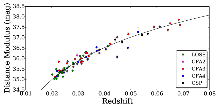
Here we show that a subset of SNe Ia, identified only from photometry of a circular 5 kpc aperture at the SN position, yield distances from optical light-curve fitting with % precision. Our sample consists of SNe Ia with and is assembled from the Lick Observatory Supernova Search (LOSS), Harvard-Smithsonian Center for Astrophysics (CfA), and Carnegie Supernova Project (CSP) collections of published light curves given in Table S1. Table S2 describes our light-curve sample selection criteria. The redshifts of the SNe place them in the Hubble flow, where galaxy peculiar velocities are substantially smaller than velocities arising from the cosmic expansion.
We computed distance moduli using the MLCS2k2 light-curve fitting algorithm (?) available as part of the SuperNova ANAlysis (SNANA; v10.35) (?) package. MLCS2k2 parameterizes light curves using a decline parameter and an extinction to the explosion , and solves simultaneously for both. Model light curves with higher values of fade more quickly and are intrinsically redder.
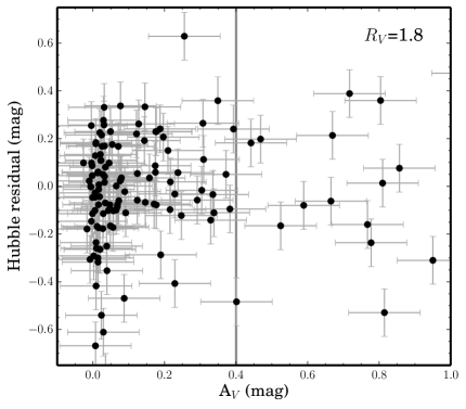
To model extinction by dust, MLCS2k2 applies the O’Donnell (?) law, parameterized by the ratio between the -band extinction and the selective extinction . Whereas this ratio has a typical value of along Milky Way sight lines (?), lower values of yield the smallest Hubble-residual scatter for nearby SNe Ia (?). A Hubble residual (HR ) is defined here as the difference between , the distance modulus to the SN inferred from the light curve, and , the distance modulus expected from the SN redshift and the best-fitting cosmological parameters. SN Ia color variation that does not correlate with brightness (?), or reddening by dust different from that along Milky-Way sight lines (?) may explain why low values of yield reduced Hubble-residual scatter. We find that the value minimizes the scatter of Hubble residuals of the SNe in our full sample, after fitting light curves with values of in mag increments.
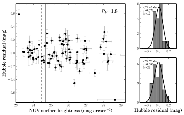
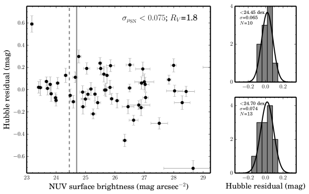
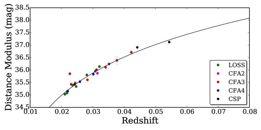
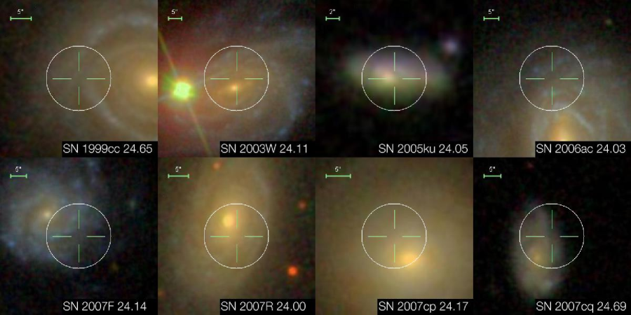
Using images taken by the GALEX satellite, we measure the host-galaxy surface brightnesses in the far- and near-ultraviolet (FUV and NUV) bandpasses within a circular 5 kpc aperture centered on the SN position. SNe Ia whose apertures have high NUV surface brightness (Fig. 1) exhibit an exceptionally small scatter among their Hubble residuals. Among the 17 SNe Ia in environments brighter than 24.45 mag arcsec-2, the root-mean-square scatter in the Hubble residuals is 0.0730.012 mag. When we examine only the 10 SNe Ia with statistical uncertainty mag for the distance modulus, the root-mean-square scatter is 0.0650.016 mag. The only SNe we excluded when we computed the sample standard deviation is SN 2007bz, which exploded in a region of high surface brightness and has an offset from the redshift-distance relation (HR mag). Although our MLCS2k2 fit to the light curve of SN 2007bz yields mag, a published BAYESN fit instead favors a higher extinction of mag (?), which would correspond to a significantly reduced Hubble residual. The redshift-distance relation constructed using only SNe Ia in environments with high NUV surface brightness exhibits significantly smaller scatter than that for the entire SNe Ia sample (Fig. 2).
To determine the statistical significance of finding a sample of SNe with Hubble-residual scatter , we performed 10,000 simulations in which we randomly shuffled the Hubble residuals of the parent SN sample, after removing outliers with mag. For each shuffled sample of SNe, we next simulated the selection of a NUV surface-brightness upper limit that minimized the Hubble-residual scatter of the sample. Searching within mag of the 24.45 mag NUV analysis upper limit in 0.05 mag increments, we identify the upper limit that minimizes the shuffled sample’s Hubble-residual scatter. The percentage of simulations that yielded a standard deviation smaller than is the value. As shown in Table 1, only 0.2% of simulated samples have a scatter smaller than the 0.0730.012 mag that we measured for SNe Ia in host environments with high UV surface brightness.
For the redshift distribution of the SNe that form the 24.45 mag NUV sample, we used Monte Carlo simulations to calculate the expected contributions of peculiar velocities to Hubble-residual scatter. We computed 0.0500.010 mag for 200 km s-1, and 0.0750.015 mag for 300 km s-1. Because the Hubble-residual scatter we measured for SNe Ia in host environments with high UV surface brightness is not much greater than that expected from peculiar motions alone, their intrinsic scatter in their luminosities after light-curve calibration is likely to be appreciably smaller than 0.08 mag (4% in distance).
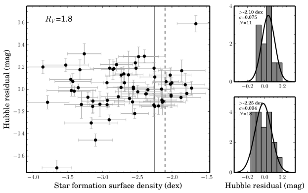
We also estimated the average star-formation surface density [solar mass (M⊙) yr-1 kpc-2] within each circular 5 kpc aperture, when both optical (ugriz or BVRI) as well as FUV and NUV imaging of the host galaxy were available. The star-formation rate is computed by comparing the observed fluxes with predictions for stellar populations having a broad range of star-formation histories. Although fewer host galaxies have the necessary imaging, Fig. 3 shows that the SNe having high star-formation density environments also have comparably small scatter in their Hubble residuals. The 11 SNe Ia with average star-formation surface density values in their apertures greater than dex exhibit 0.0750.018 mag. Among randomly shuffled samples, only 1.1% have a smaller standard deviation among their Hubble residuals, after searching within dex of the dex limit.
The 10 kpc diameter of the host-galaxy aperture subtends an angle of at and at . Therefore, for future cosmological analyses, the NUV surface brightnesses of high-redshift SN Ia hosts within a circular 5 kpc aperture can be measured from the ground in conditions with sub-arcsecond seeing, making possible precise measurements of distances to high redshift.
The large UV surface brightnesses and star-formation densities of the environments of highly standardizable SNe Ia, as well as the star formation evident from Sloan Digital Sky Survey (SDSS) images, reveal the existence of young, massive stars. A reasonable conclusion is that the delay between the birth of the SN precursor and its explosion as a white dwarf is comparatively short.
The SDSS composite images in Fig. S6 show that the 5 kpc apertures include stellar populations of multiple ages, and the younger stellar populations are expected to dominate the measured NUV flux. While O-type and early B-type stars of masses are required to produce the ionizing radiation responsible for H ii regions, stars with masses of having lifetimes of million years are responsible for the UV luminosity (?, ?). A delay time of million years would be required for a SN Ia progenitor to travel kpc with a natal velocity of 10 km s-1.
The total mass, metallicity, central density, and carbon-to-oxygen ratio of the white dwarf, as well as the properties of the binary companion, probably vary within the progenitor population of SNe Ia. In theoretical simulations of both single-degenerate (?, ?, ?) and double-degenerate (?, ?) explosions, the variation of many of these parameters can yield a correlation between light-curve decline rate and luminosity, but the normalization and slope of these predicted correlations generally show significant differences. Therefore, it is likely that variations in one, or possibly two, progenitor properties contribute significantly to the light-curve width/color/luminosity relation of the highly standardizable SNe Ia population. The asymmetry of the explosion, which is thought to increase random scatter around the light-curve width/color/luminosity relation, may be small within this population and may possibly indicate that most burning occurs during the detonation phase (?). A reasonable possibility is that the relatively young ages of the progenitor population correspond to a population with a smaller dispersion in their ages, leading to more uniform calibration.
As we show in Table 1, for both the full sample and the SNe found in UV-bright environments, MLCS2k2 distances computed with yield a smaller Hubble-residual scatter than those computed with . Although the low apparent value of may result in part from color variation unconnected to SN brightness (?), polarization data suggest that dust properties may also be important. For a handful of well-sampled SNe Ia where the extinction is large ( mag), the small intrinsic continuum polarization (%) of SNe Ia (?) allows constraints on the wavelength-dependent polarization introduced by intervening dust (?). Analyses of SN 1986G, SN 2006X, SN 2008fp, and SN 2014J show evidence for low values of and blue polarization peaks, consistent with a small grain size distribution (?). In these cases, the polarization vector is aligned with the apparent local spiral arm structure, suggesting that the dust is interstellar rather than circumstellar.
A possibility is that SN environments exhibiting intense star formation may generate outflowing winds that entrain small dust grains, which might explain the evidence for low and the continuum polarization. Dust particles in the SN-driven superwind emerging from the nearby starburst galaxy M82 scatter light that originates in the star-forming disk, and the spectral energy distribution of the scattered light is consistent with a comparatively small grain size distribution (?).
References and Notes
- 1. M. M. Phillips “The absolute magnitudes of Type IA supernovae” In ApJ 413, 1993, pp. L105–L108 DOI: 10.1086/186970
- 2. A. G. Riess, W. H. Press and R. P. Kirshner “A Precise Distance Indicator: Type IA Supernova Multicolor Light-Curve Shapes” In ApJ 473, 1996, pp. 88 DOI: 10.1086/178129
- 3. A. G. Riess et al. “Observational Evidence from Supernovae for an Accelerating Universe and a Cosmological Constant” In AJ 116, 1998, pp. 1009–1038 DOI: 10.1086/300499
- 4. S. Perlmutter et al. “Measurements of Omega and Lambda from 42 High-Redshift Supernovae” In ApJ 517, 1999, pp. 565–586 DOI: 10.1086/307221
- 5. D. O. Jones et al. “The Discovery of the Most Distant Known Type Ia Supernova at Redshift 1.914” In ApJ 768, 2013, pp. 166 DOI: 10.1088/0004-637X/768/2/166
- 6. D. H. Weinberg et al. “Observational probes of cosmic acceleration” In Phys. Rep. 530, 2013, pp. 87–255 DOI: 10.1016/j.physrep.2013.05.001
- 7. P. L. Kelly et al. “Hubble Residuals of Nearby Type Ia Supernovae are Correlated with Host Galaxy Masses” In ApJ 715, 2010, pp. 743–756 DOI: 10.1088/0004-637X/715/2/743
- 8. M. Sullivan et al. “The dependence of Type Ia Supernovae luminosities on their host galaxies” In MNRAS 406, 2010, pp. 782–802 DOI: 10.1111/j.1365-2966.2010.16731.x
- 9. H. Lampeitl et al. “The Effect of Host Galaxies on Type Ia Supernovae in the SDSS-II Supernova Survey” In ApJ 722, 2010, pp. 566–576 DOI: 10.1088/0004-637X/722/1/566
- 10. M. Childress et al. “Host Galaxy Properties and Hubble Residuals of Type Ia Supernovae from the Nearby Supernova Factory” In ApJ 770, 2013, pp. 108 DOI: 10.1088/0004-637X/770/2/108
- 11. M. Rigault et al. “Evidence of environmental dependencies of Type Ia supernovae from the Nearby Supernova Factory indicated by local H” In A&A 560, 2013, pp. A66 DOI: 10.1051/0004-6361/201322104
- 12. X. Wang et al. “Improved Distances to Type Ia Supernovae with Two Spectroscopic Subclasses” In ApJ 699, 2009, pp. L139–L143 DOI: 10.1088/0004-637X/699/2/L139
- 13. R. J. Foley and D. Kasen “Measuring Ejecta Velocity Improves Type Ia Supernova Distances” In ApJ 729, 2011, pp. 55 DOI: 10.1088/0004-637X/729/1/55
- 14. S. Bailey et al. “Using spectral flux ratios to standardize SN Ia luminosities” In A&A 500, 2009, pp. L17–L20 DOI: 10.1051/0004-6361/200911973
- 15. S. Blondin, K. S. Mandel and R. P. Kirshner “Do spectra improve distance measurements of Type Ia supernovae?” In A&A 526, 2011, pp. A81 DOI: 10.1051/0004-6361/201015792
- 16. J. M. Silverman, M. Ganeshalingam, W. Li and A. V. Filippenko “Berkeley Supernova Ia Program - III. Spectra near maximum brightness improve the accuracy of derived distances to Type Ia supernovae” In MNRAS 425, 2012, pp. 1889–1916 DOI: 10.1111/j.1365-2966.2012.21526.x
- 17. K. S. Mandel, R. J. Foley and R. P. Kirshner “Type Ia Supernova Colors and Ejecta Velocities: Hierarchical Bayesian Regression with Non-Gaussian Distributions” In ApJ 797, 2014, pp. 75 DOI: 10.1088/0004-637X/797/2/75
- 18. W. M. Wood-Vasey et al. “Type Ia Supernovae Are Good Standard Candles in the Near Infrared: Evidence from PAIRITEL” In ApJ 689, 2008, pp. 377–390 DOI: 10.1086/592374
- 19. K. S. Mandel, G. Narayan and R. P. Kirshner “Type Ia Supernova Light Curve Inference: Hierarchical Models in the Optical and Near-infrared” In ApJ 731, 2011, pp. 120 DOI: 10.1088/0004-637X/731/2/120
- 20. A. G. Kim et al. “Standardizing Type Ia Supernova Absolute Magnitudes Using Gaussian Process Data Regression” In ApJ 766, 2013, pp. 84 DOI: 10.1088/0004-637X/766/2/84
- 21. S. Jha, A. G. Riess and R. P. Kirshner “Improved Distances to Type Ia Supernovae with Multicolor Light-Curve Shapes: MLCS2k2” In ApJ 659, 2007, pp. 122–148 DOI: 10.1086/512054
- 22. R. Kessler et al. “SNANA: A Public Software Package for Supernova Analysis” In PASP 121, 2009, pp. 1028–1035 DOI: 10.1086/605984
- 23. J. E. O’Donnell “R_nu-dependent optical and near-ultraviolet extinction” In ApJ 422, 1994, pp. 158–163 DOI: 10.1086/173713
- 24. E. L. Fitzpatrick and D. Massa “An Analysis of the Shapes of Interstellar Extinction Curves. V. The IR-through-UV Curve Morphology” In ApJ 663, 2007, pp. 320–341 DOI: 10.1086/518158
- 25. M. Hicken et al. “Improved Dark Energy Constraints from ~100 New CfA Supernova Type Ia Light Curves” In ApJ 700, 2009, pp. 1097–1140 DOI: 10.1088/0004-637X/700/2/1097
- 26. D. M. Scolnic et al. “Color Dispersion and Milky-Way-like Reddening among Type Ia Supernovae” In ApJ 780, 2014, pp. 37 DOI: 10.1088/0004-637X/780/1/37
- 27. F. Patat et al. “Properties of extragalactic dust inferred from linear polarimetry of Type Ia Supernovae” In ArXiv e-prints, 2014 arXiv:1407.0136
- 28. S. G. Stewart et al. “Star Formation Triggering Mechanisms in Dwarf Galaxies: The Far-Ultraviolet, H, and H I Morphology of Holmberg II” In ApJ 529, 2000, pp. 201–218 DOI: 10.1086/308241
- 29. S. M. Gogarten et al. “The ACS Nearby Galaxy Survey Treasury. II. Young Stars and their Relation to H and UV Emission Timescales in the M81 Outer Disk” In ApJ 691, 2009, pp. 115–130 DOI: 10.1088/0004-637X/691/1/115
- 30. S. E. Woosley, D. Kasen, S. Blinnikov and E. Sorokina “Type Ia Supernova Light Curves” In ApJ 662, 2007, pp. 487–503 DOI: 10.1086/513732
- 31. D. Kasen, F. K. Röpke and S. E. Woosley “The diversity of type Ia supernovae from broken symmetries” In Nature 460, 2009, pp. 869–872 DOI: 10.1038/nature08256
- 32. S. A. Sim et al. “Synthetic light curves and spectra for three-dimensional delayed-detonation models of Type Ia supernovae” In MNRAS 436, 2013, pp. 333–347 DOI: 10.1093/mnras/stt1574
- 33. D. Kushnir et al. “Head-on Collisions of White Dwarfs in Triple Systems Could Explain Type Ia Supernovae” In ApJ 778, 2013, pp. L37 DOI: 10.1088/2041-8205/778/2/L37
- 34. R. Moll, C. Raskin, D. Kasen and S. E. Woosley “Type Ia Supernovae from Merging White Dwarfs. I. Prompt Detonations” In ApJ 785, 2014, pp. 105 DOI: 10.1088/0004-637X/785/2/105
- 35. L. Wang and J. C. Wheeler “Spectropolarimetry of Supernovae” In ARA&A 46, 2008, pp. 433–474 DOI: 10.1146/annurev.astro.46.060407.145139
- 36. S. Hutton et al. “A panchromatic analysis of starburst galaxy M82: probing the dust properties” In MNRAS 440, 2014, pp. 150–160 DOI: 10.1093/mnras/stu185
- 37. A. U. Landolt “UBVRI photometric standard stars in the magnitude range 11.5-16.0 around the celestial equator” In AJ 104, 1992, pp. 340–371 DOI: 10.1086/116242
- 38. D. J. Fixsen et al. “The Cosmic Microwave Background Spectrum from the Full COBE FIRAS Data Set” In ApJ 473, 1996, pp. 576 DOI: 10.1086/178173
- 39. E. F. Schlafly and D. P. Finkbeiner “Measuring Reddening with Sloan Digital Sky Survey Stellar Spectra and Recalibrating SFD” In ApJ 737, 2011, pp. 103 DOI: 10.1088/0004-637X/737/2/103
- 40. P. Nugent, A. Kim and S. Perlmutter “K-Corrections and Extinction Corrections for Type Ia Supernovae” In PASP 114, 2002, pp. 803–819 DOI: 10.1086/341707
- 41. R. R. Gupta et al. “Improved Constraints on Type Ia Supernova Host Galaxy Properties Using Multi-wavelength Photometry and Their Correlations with Supernova Properties” In ApJ 740, 2011, pp. 92 DOI: 10.1088/0004-637X/740/2/92
- 42. C. B. D’Andrea et al. “Spectroscopic Properties of Star-forming Host Galaxies and Type Ia Supernova Hubble Residuals in a nearly Unbiased Sample” In ApJ 743, 2011, pp. 172 DOI: 10.1088/0004-637X/743/2/172
- 43. J. Johansson et al. “SN Ia host galaxy properties from Sloan Digital Sky Survey-II spectroscopy” In MNRAS 435, 2013, pp. 1680–1700 DOI: 10.1093/mnras/stt1408
- 44. B. T. Hayden et al. “The Fundamental Metallicity Relation Reduces Type Ia SN Hubble Residuals More than Host Mass Alone” In ApJ 764, 2013, pp. 191 DOI: 10.1088/0004-637X/764/2/191
- 45. Y.-C. Pan et al. “The host galaxies of Type Ia supernovae discovered by the Palomar Transient Factory” In MNRAS 438, 2014, pp. 1391–1416 DOI: 10.1093/mnras/stt2287
- 46. E. Bertin and S. Arnouts “SExtractor: Software for source extraction.” In AJ 117, 1996, pp. 393–404
- 47. A. V. Filippenko, W. D. Li, R. R. Treffers and M. Modjaz “The Lick Observatory Supernova Search with the Katzman Automatic Imaging Telescope” In Small Telescope Astronomy on Global Scales 246 San Francisco: ASP, 2001, pp. 121
- 48. M. Ganeshalingam et al. “Results of the Lick Observatory Supernova Search Follow-up Photometry Program: BVRI Light Curves of 165 Type Ia Supernovae” In ApJS 190, 2010, pp. 418–448 DOI: 10.1088/0067-0049/190/2/418
- 49. D. Lang et al. “Astrometry.net: Blind Astrometric Calibration of Arbitrary Astronomical Images” In AJ 139, 2010, pp. 1782–1800 DOI: 10.1088/0004-6256/139/5/1782
- 50. E. Bertin “Automatic Astrometric and Photometric Calibration with SCAMP” In Astronomical Data Analysis Software and Systems XV 351, Astronomical Society of the Pacific Conference Series, 2006, pp. 112
- 51. M. F. Skrutskie et al. “The Two Micron All Sky Survey (2MASS)” In AJ 131, 2006, pp. 1163–1183 DOI: 10.1086/498708
- 52. E. Bertin et al. “The TERAPIX Pipeline” In Astronomical Data Analysis Software and Systems XI, 2002, pp. 228
- 53. E. Bertin “Automated Morphometry with SExtractor and PSFEx” In Astronomical Data Analysis Software and Systems XX 442, Astronomical Society of the Pacific Conference Series, 2011, pp. 435
- 54. P. L. Kelly et al. “Weighing the Giants - II. Improved calibration of photometry from stellar colours and accurate photometric redshifts” In MNRAS 439, 2014, pp. 28–47 DOI: 10.1093/mnras/stt1946
- 55. D. C. Martin et al. “The Galaxy Evolution Explorer: A Space Ultraviolet Survey Mission” In ApJ 619, 2005, pp. L1–L6 DOI: 10.1086/426387
- 56. M. R. Blanton and S. Roweis “K-Corrections and Filter Transformations in the Ultraviolet, Optical, and Near-Infrared” In AJ 133, 2007, pp. 734–754 DOI: 10.1086/510127
- 57. M. Fioc and B. Rocca-Volmerange “PEGASE.2, a metallicity-consistent spectral evolution model of galaxies: the documentation and the code” In ArXiv Astrophysics e-prints, 1999 eprint: astro-ph/9912179
- 58. J. Leaman, W. Li, R. Chornock and A. V. Filippenko “Nearby supernova rates from the Lick Observatory Supernova Search - I. The methods and data base” In MNRAS 412, 2011, pp. 1419–1440 DOI: 10.1111/j.1365-2966.2011.18158.x
- 59. W. Li et al. “Nearby supernova rates from the Lick Observatory Supernova Search - II. The observed luminosity functions and fractions of supernovae in a complete sample” In MNRAS 412, 2011, pp. 1441–1472 DOI: 10.1111/j.1365-2966.2011.18160.x
- 60. S. Jha et al. “UBVRI Light Curves of 44 Type Ia Supernovae” In AJ 131, 2006, pp. 527–554 DOI: 10.1086/497989
- 61. M. Hicken et al. “CfA3: 185 Type Ia Supernova Light Curves from the CfA” In ApJ 700, 2009, pp. 331–357 DOI: 10.1088/0004-637X/700/1/331
- 62. M. Hicken et al. “CfA4: Light Curves for 94 Type Ia Supernovae” In ApJS 200, 2012, pp. 12 DOI: 10.1088/0067-0049/200/2/12
- 63. C. Contreras et al. “The Carnegie Supernova Project: First Photometry Data Release of Low-Redshift Type Ia Supernovae” In AJ 139, 2010, pp. 519–539 DOI: 10.1088/0004-6256/139/2/519
- 64. M. D. Stritzinger et al. “The Carnegie Supernova Project: Second Photometry Data Release of Low-redshift Type Ia Supernovae” In AJ 142, 2011, pp. 156 DOI: 10.1088/0004-6256/142/5/156
Acknowledgements
We thank S. Sim, J. C. Wheeler, J. Silverman, A. Conley, M. Graham, D. Kasen, I. Shivvers, and R. Kessler for useful discussions and comments on the paper, and J. Schwab for his help providing background about theoretical modeling. We are grateful to the staffs at Lick Observatory and Kitt Peak National Observatory (KPNO) for their assistance. The late Weidong Li was instrumental to the success of LOSS. A.V.F.’s supernova group at the University of California Berkeley has received generous financial assistance from the Christopher R. Redlich Fund, the TABASGO Foundation, and NSF grant AST-1211916. The Katzman Automatic Imaging Telescope and its ongoing operation were made possible by donations from Sun Microsystems, the Hewlett-Packard Company, AutoScope Corporation, Lick Observatory, NSF, the University of California, the Sylvia and Jim Katzman Foundation, and the TABASGO Foundation. The SLAC Department of Energy contract number is DE-AC02-76SF00515. GALEX data are available from http://galex.stsci.edu/GR6/, SDSS data may be obtained at http://www.sdss.org, the KPNO imaging is archived at http://portal-nvo.noao.edu, and the Lick Observatory images are available from http://astro.berkeley.edu/bait/public_html/iahostpaper/.
| Criterion | () | () |
|---|---|---|
| UV and | 0.1280.014 (50) | 0.1310.015 (46) |
| NUV SB 24.45 | 0.0650.016 (10; 1.1%) | 0.0940.027 (8; 24%) |
| NUV SB 24.7 | 0.0740.012 (13; 1.2%) | 0.0870.019 (13; 17%) |
| Full UV Sample | 0.1300.010 (77) | 0.1380.008 (78) |
| NUV SB 24.45 | 0.0730.012 (17; 0.2%) | 0.0900.014 (17; 1.1%) |
| NUV SB 24.7 | 0.0830.012 (22; 0.3%) | 0.0890.010 (24; 0.6%) |
| Full SFR Sample | 0.1330.012 (61) | 0.1390.012 (62) |
| 0.0750.018 (11; 1.1%) | 0.0810.016 (11; 1.3%) | |
| 0.0940.015 (18; 1.8%) | 0.1020.015 (18; 2.6%) |
Supplementary Materials
This PDF file includes the following:
-
Material and Methods
-
Supplementary Text
-
Figures S1 to S7
-
Tables S1 to S4
-
References 37–64
Materials and Methods
Selection of Light Curves.
To include a SN in our sample, we require a photometric measurement before 5 days after B-band maximum, at least one photometric measurement after B-band maximum, and at least three separate epochs having a signal-to-noise ratio (S/N) measurement. Only photometry through 50 days after B-band maximum enters the fitting with MLCS2k2.
A fraction of the SNe in our sample were followed by multiple teams and published in more than one of the light-curve collections listed in Table S1. We selected the light curve according to the order in Table S1, with light-curve collections at the beginning of the list having precedence. Rearranging the order does not significantly change the Hubble-residual statistics that we measure.
MLCS2k2 Light-Curve Fitting.
Except for CSP SN Ia photometry, for which we use magnitudes in the natural system, all fitting is performed to fluxes in the Landolt standard system (?). Heliocentric SN Ia redshifts are transformed to the cosmic microwave background (CMB) rest frame using the dipole velocity (?). We correct fluxes for Milky Way extinction (?) using the O’Donnell 1994 reddening law (?). Since MLCS2k2 performs light-curve fitting to rest-frame fluxes, the observed SN fluxes are transformed, prior to fitting, from the observer frame into the rest frame using a K-correction (?). When performing MLCS2k2 fitting using SNANA, we apply an exponential prior on with mag (PRIOR_AVEXP ) convolved with a Gaussian kernel having mag (PRIOR_AVRES 0.02). We obtain similar Hubble-residual scatter among SNe in UV-bright environments when priors instead with mag and mag are used while fitting.
To calculate the Hubble residuals of individual SNe, we first find the redshift-distance relation that minimizes the value of the fit to the MLCS2k2 distance moduli. For the purpose of fitting for the redshift-distance relation, we add an uncertainty of 0.07 mag in quadrature to the statistical uncertainty on each distance computed by MLCS2k2. After minimizing the value, we repeat the fit with only the SNe having Hubble residuals smaller than 0.3 mag. The best-fitting relation is not significantly affected by the specific values of the additional uncertainty, or of the criterion used to identify outlying SNe.
Figures S2 and S3 show the light-curve parameter cuts that we apply to the sample of SN Ia light curves. A principal purpose of light-curve cuts used in cosmological analyses is to remove SNe that may be systematically offset from the light-curve width/color/luminosity relation, that show extremely large dispersion around the redshift-distance relation, or that have light curves that indicate high reddening. As Figs. S2 and S3 show, we selected light-curve cuts that achieved these aims.
As Figure S3 shows, fast-declining () SNe Ia in our sample are absent from UV-bright host-galaxy environments. Since these fast-declining SNe have Hubble residuals that are systematically low (Fig. S2), including these SNe in our analysis sample would increase the Hubble-residual scatter of the full SN Ia sample, but not affect the UV-bright subset. Therefore, the addition of the fast-declining SNe would increase the statistical significance of the comparatively small Hubble-residual scatter we observe among SNe in UV-bright regions. Nonetheless, we exclude the fast-declining SNe to show that SNe Ia having typical light curves exhibit a smaller Hubble-residual scatter, when found in regions having high UV brightness.
Calculating Statistical Significance.
Through Monte Carlo simulations, we have assessed the probability that the small Hubble-residual scatter we measure for SNe Ia in UV-bright host-galaxy apertures is only a random effect. An additional possibility is that, from random effects, the SNe erupting instead, for example, in UV-faint regions could have exhibited small apparent Hubble-residual scatter. If we expect that we would have reported such an alternative pattern as a discovery, then the -values we compute should be adjusted to account for multiple searches. For separate searches, the probability of finding at least one random pattern having significance is . We have calculated, assuming a single search, a -value of 0.2% for the measured Hubble-residual scatter of 0.0730.012 mag for SNe Ia in regions with high NUV surface brightness (see Table 1). Assuming instead separate searches, for example, would yield an adjusted -value of 0.8%.
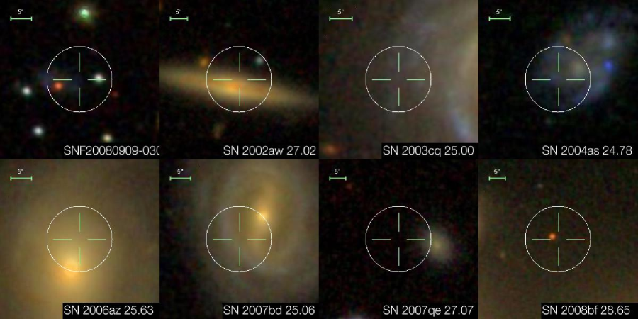
However, a principal focus of our analysis from its inception was to identify SNe Ia in UV-bright, star-forming environments using GALEX imaging, motivated by a recent analysis of H flux near explosion sites (?). Indeed, while high UV surface brightness within the 5 kpc aperture provides strong evidence for a young stellar population, interpretation of low average UV surface brightness is less straightforward. As shown in Figure S6, the apertures with lower NUV surface brightness consist of a heterogeneous mix of SNe in low-mass galaxies having small physical sizes, SNe with large host offsets, and SNe erupting in old stellar populations. Given the mixed set of environments, it probably would have been unlikely that we would feel we had found a robust pattern. If SNe with very small scatter exploded from the oldest stellar populations, we also note that such an association probably would already have been identified using the host-galaxy morphology, spectroscopy, or optical and infrared photometry (?, ?, ?, ?, ?, ?, ?).
KPNO Image Reduction and Calibration.
We acquired ugriz imaging of SN Ia host galaxies with the T2KA and T2KB cameras mounted on the Kitt Peak National Observatory (KPNO) 2.1 m telescope in June 2009, March 2010, May 2010, October 2010, and December 2010. The raw images were processed using standard IRAF222http://iraf.noao.edu/ reduction routines. A master bias frame was created from the median stack of the bias exposures taken each night, and subtracted from the flat field and from images of the host galaxies. For each run, we constructed a median dome-flat exposure that we used to correct the host-galaxy images. To improve the flat-field correction, a median stack of all host-galaxy frames was computed after removing all objects detected using SExtractor (?).
Even after dividing images by the flat field and by stacked, object-subtracted science images, the edge to the south of the T2KB CCD array showed a % spatially dependent background variation. To remove this poorly corrected region of the detector, we trimmed the 400 pixel columns closest to south edge of the T2KB pixel array, after overscan subtraction. We constructed a fringe model for z-band images from object-subtracted science images, and scaled the model to best remove fringing from the affected images.
Lick Observatory Image Reduction and Calibration.
We used the bias and flat-field corrected BVRI “template” images of the host galaxies of SNe Ia acquired after the SNe had faded, as part of the LOSS follow-up program (?). The imaging was obtained using the 0.76 m Katzman Automatic Imaging Telescope (KAIT) and the 1 m Anna Nickel telescope at Lick Observatory (?). During the period when the observations were taken, the CCD detector that was mounted on KAIT was replaced twice, while the BVRI filter set was replaced once.
Astrometric and Photometric Calibration of KPNO and Lick Observatory Imaging.
We used the Astrometry.net routine (?), which matches sources in each input image against positions in the USNO-B catalog, to generate a World Coordinate System (WCS) for each KPNO 2.1 m, KAIT, and Nickel image. After updating each image with the WCS computed by Astrometry.net, we performed a simultaneous astrometric fit that included every exposure of each host galaxy across all passbands using the SCAMP package (?), and the 2MASS (?) point-source catalog as the reference.
The resulting WCS solution was passed to SWarp (?) and used to resample all images to a common pixel grid. To extract stellar magnitudes, we next used SExtractor (?) to measure magnitudes inside circular apertures with radius. PSFEx (?) was used to fit a Moffat point-spread function (PSF) model and calculate an aperture correction for each image. We computed ugriz or BVRI zeropoints from the stellar locus using the publicly available big macs333https://code.google.com/p/big-macs-calibrate/ package developed by the authors (?). The routine synthesizes the expected stellar locus for an instrument and detector combination using the wavelength-dependent transmission and a spectroscopic model of the SDSS stellar locus.
Host-Galaxy Photometry.
To measure UV emission from host galaxies, we used both FUV and NUV imaging from the All-Sky Imaging Survey and Medium Imaging Survey performed by the GALEX (?) satellite. The GALEX FUV passband has a central wavelength of 1528 Å and a PSF full width at half-maximum intensity (FWHM) of , while the central wavelength of the NUV passband is 2271 Å and the PSF FWHM is . Photometry at optical wavelengths was measured from ugriz images taken with the SDSS or the KPNO 2.1 m telescope, or from BVRI images taken with KAIT or the 1 m Nickel telescope at Lick Observatory. All optical images were convolved to have a PSF of to match that of the GALEX NUV images before extracting host-galaxy photometry.
When assembling mosaics of host-galaxy images, we record the MJD of each image. We exclude exposures taken from between two weeks prior to through 210 days past the date when the SN reached B-band maximum. For the SN host galaxies that have images without contaminating flux, we resample all exposures to a common grid centered on the SN explosion coordinates using the SWarp software program. We measure the host-galaxy flux within a circular 5 kpc aperture, and compute K-corrections using kcorrect (?). If the uncertainty of a magnitude in a specific bandpass exceeds 0.3 mag, then we use the magnitude synthesized from the kcorrect model that best fits the full set of measured magnitudes, instead of adding a K-correction to the measured magnitude. We adjust surface-brightness estimates calculated from K-corrected magnitudes for cosmological dimming. When both UV and optical host photometry are available, we estimate the star-formation surface density using the PEGASE2 (?) stellar population synthesis models. In Table S4, we list measured light-curve parameters, host-galaxy measurements, and Hubble residuals.
Supplementary Text
Additional Evidence for a Low-Scatter Population from SNe with Multiple Light Curves.
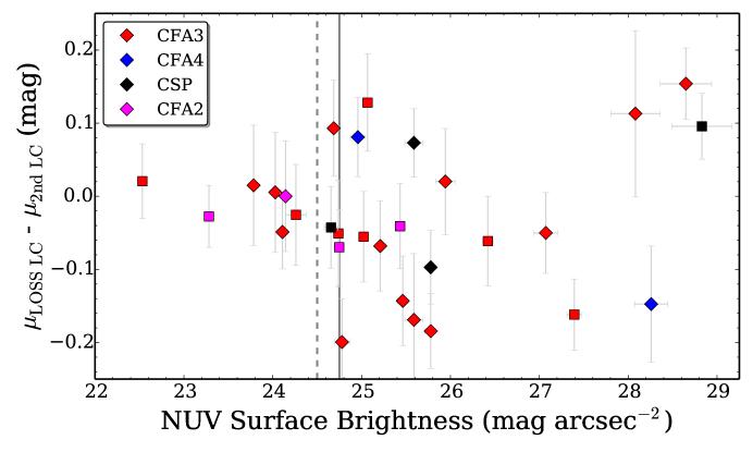
A fraction of SNe have separate light-curve measurements published in the LOSS collection as well as in a second collection of light curves (CfA2, CfA3, CfA4, or CSP). After completing an advanced draft of the paper, we compared the pairs of MLCS2k2 distance moduli to these SNe. Since these distances are not affected by the peculiar motion of the host galaxies (unlike ), we can additionally study SNe which are not part of the Hubble-residual sample. Figure S1 shows that there is greater agreement between the distance moduli to the SNe Ia that explode in regions with high NUV surface brightness. This provides additional evidence, discovered after identifying the low-scatter population, that SNe Ia in UV-bright regions yield more precise distances.
and the Hubble Residuals of SNe in Regions with High NUV Surface Brightness.
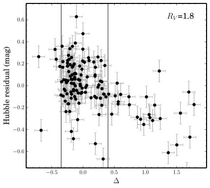
Figure S5 shows Hubble residuals against for MLCS2k2 distance moduli computed using and .
FUV Surface Brightness.
Figure S4 shows that the FUV surface brightness yields comparably small Hubble-residual scatter as NUV surface brightness. Among the Hubble residuals of the 17 SNe Ia in environments brighter than 24.9 mag arcsec-2, the root-mean-square scatter is 0.0740.012 mag. When we examine only the 10 SNe Ia with distance modulus statistical uncertainty mag, the root-mean-square scatter is 0.0670.014 mag. Additional statistics are listed in Table 1.
Color-Composite Images of Explosion Environments.
Figure S6 displays panels of SDSS color-composite images of the host-galaxy environments for SNe Ia whose circular 5 kpc apertures have high or low average NUV surface brightness. These images show that SNe that occur within the host-galaxy outskirts, as well as in small low-mass galaxies, have low average NUV surface brightness within the aperture.
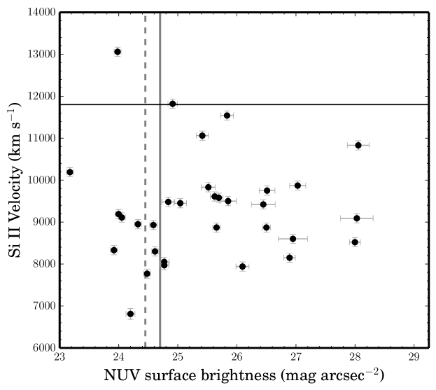
Si II Velocity.
In Figure S7, we show the velocities of SNe Ia that have Si ii measurements within seven days of B-band maximum brightness against NUV surface brightness within the circular 5 kpc aperture. The highly standardizable population found in high surface brightness regions shows no strong differences in the distributions of Si ii velocities near maximum brightness.
| Light-Curve Dataset | Filters | References |
|---|---|---|
| Lick Observatory Supernova Search (LOSS) | BVRI | (?, ?, ?) |
| CfA2 | (U)BVRI | (?) |
| CfA3 | (U)BVRIr’i’ | (?) |
| CfA4 | (U)BVr’i’ | (?) |
| Carnegie Supernova Project (CSP) | (u)BVgri | (?, ?) |
| Criterion | SNe |
|---|---|
| 307 | |
| 292 | |
| 165 | |
| mag | 143 |
| 107 | |
| MLCS2k2 | 107 |
| Not SNF20080522-000 | 106 |
| MW mag | 103 |
| Uncontaminated FUV; NUV | 83 |
| Hubble residual mag | 77 |
| Uncontaminated FUV; NUV; ugriz or BVRI | 67 |
| Hubble residual mag | 61 |
| Name | FUV SB | NUV SB | SFR Density | HR | HR | |
|---|---|---|---|---|---|---|
| mag arcsec-2 | mag arcsec-2 | dex | = 1.8 | = 3.1 | ||
| SN 1997dg | 0.034 | 25.720.19 | 25.820.10 | -2.480.29 | 0.290.09 | 0.040.11 |
| SN 1999cc | 0.031 | 25.330.17 | 24.480.08 | -2.140.33 | -0.120.12 | -0.100.12 |
| SN 1999dg | 0.022 | 27.89 (model) | 26.100.11 | -2.770.25 | -0.070.09 | -0.030.09 |
| SN 2000dn | 0.032 | 27.61 (model) | 26.950.25 | -2.840.29 | 0.190.06 | 0.220.06 |
| SN 2000fa | 0.021 | 25.020.08 | 24.000.06 | -2.150.21 | -0.100.05 | -0.130.06 |
| SN 2001br | 0.021 | 27.17 (model) | 26.510.13 | -2.800.23 | 0.220.06 | 0.210.07 |
| SN 2001cj | 0.024 | 28.630.26 | 27.840.07 | -3.460.30 | 0.090.04 | 0.130.04 |
| SN 2001ck | 0.035 | 24.110.13 | 23.710.08 | -1.720.26 | 0.010.06 | 0.050.06 |
| SN 2001cp | 0.022 | 28.13 (model) | 28.030.28 | -3.450.35 | -0.010.05 | 0.000.06 |
| SN 2001ie | 0.031 | 29.23 (model) | 28.230.30 | -3.300.25 | -0.140.13 | -0.200.15 |
| SN 2002aw | 0.026 | 27.53 (model) | 26.890.10 | . . . | -0.160.07 | -0.240.09 |
| SN 2002de | 0.028 | 24.180.06 | 23.670.06 | . . . | 0.070.04 | 0.040.05 |
| SN 2002eb | 0.028 | 28.17 (model) | 26.500.07 | -3.350.28 | 0.010.03 | -0.000.04 |
| SN 2002el | 0.030 | 28.81 (model) | 27.510.29 | -3.160.38 | -0.300.05 | -0.270.05 |
| SN 2002hu | 0.037 | 26.90 (model) | 26.450.20 | -3.140.25 | -0.150.06 | -0.120.07 |
| SN 2003U | 0.028 | 25.100.05 | 24.610.06 | -2.260.30 | -0.140.10 | -0.120.10 |
| SN 2003W | 0.020 | 24.600.08 | 23.980.06 | -1.870.29 | -0.070.04 | -0.110.05 |
| SN 2003ch | 0.025 | 29.32 (model) | 28.15 (model) | -3.320.20 | 0.180.09 | 0.210.09 |
| SN 2003cq | 0.033 | 25.610.28 | 24.840.11 | -2.190.27 | -0.150.08 | -0.200.09 |
| SN 2003gn | 0.035 | 26.52 (model) | 25.520.12 | -2.520.36 | 0.190.06 | 0.140.06 |
| SN 2003kc | 0.033 | 24.150.06 | 23.740.06 | . . . | -0.060.13 | -0.110.20 |
| SN 2004as | 0.031 | 25.090.16 | 24.650.09 | -2.250.21 | 0.110.05 | 0.050.05 |
| SN 2004at | 0.022 | 26.480.05 | 25.890.06 | -2.610.35 | -0.080.05 | -0.040.05 |
| SN 2004bg | 0.021 | 25.770.04 | 25.080.06 | -2.380.34 | -0.040.05 | -0.000.05 |
| SN 2004br | 0.023 | 28.04 (model) | 26.640.15 | -2.900.24 | -0.270.04 | -0.230.05 |
| SN 2004bw | 0.021 | 25.090.06 | 24.480.06 | -2.010.31 | -0.050.06 | -0.020.06 |
| SN 2004ef | 0.031 | 26.400.24 | 25.410.10 | . . . | -0.120.05 | -0.160.05 |
| SN 2004gu | 0.045 | 27.77 (model) | 27.040.10 | -3.210.14 | -0.070.05 | -0.150.06 |
| SN 2005ag | 0.079 | 28.44 (model) | 26.81 (model) | -2.930.25 | -0.140.04 | -0.180.05 |
| SN 2005bg | 0.023 | 23.960.06 | 23.410.06 | . . . | 0.020.05 | 0.040.06 |
| SN 2005eq | 0.030 | 25.880.09 | 25.660.06 | -2.350.33 | -0.000.05 | -0.030.06 |
| SN 2005eu | 0.035 | 25.400.08 | 25.320.06 | -2.370.24 | -0.040.06 | 0.000.06 |
| SN 2005hc | 0.046 | 25.570.07 | 25.500.06 | -2.530.27 | 0.240.05 | 0.280.06 |
| SN 2005iq | 0.034 | 25.930.28 | 25.850.14 | . . . | 0.220.05 | 0.250.05 |
| SN 2005ku | 0.050 | 24.290.04 | 23.780.06 | -1.860.34 | 0.170.10 | 0.140.13 |
| SN 2005ms | 0.025 | 29.04 (model) | 28.000.09 | -3.530.33 | 0.220.06 | 0.250.07 |
| SN 2006S | 0.032 | 25.110.18 | 25.040.11 | -2.260.25 | 0.190.05 | 0.160.07 |
| SN 2006ac | 0.023 | 24.400.07 | 23.920.06 | -1.810.28 | 0.040.10 | 0.080.11 |
| SN 2006an | 0.064 | 27.13 (model) | 27.00 (model) | -3.430.26 | 0.070.07 | 0.110.07 |
| SN 2006az | 0.031 | 26.580.30 | 25.260.09 | -2.540.20 | -0.220.05 | -0.180.05 |
| SN 2006cf | 0.042 | 24.840.14 | 24.200.08 | -2.080.18 | 0.070.09 | 0.110.09 |
| SN 2006cj | 0.067 | 25.850.13 | 25.620.07 | -2.690.12 | 0.140.07 | 0.180.07 |
| SN 2006cp | 0.022 | 26.240.25 | 25.830.11 | -2.560.29 | 0.020.06 | -0.010.07 |
| SN 2006cq | 0.048 | 26.410.15 | 25.690.07 | -2.850.17 | 0.180.09 | 0.170.11 |
| SN 2006en | 0.032 | 24.430.10 | 23.470.06 | . . . | 0.020.07 | -0.060.09 |
| SN 2006et | 0.022 | 27.30 (model) | 26.100.11 | . . . | 0.010.10 | -0.060.12 |
| SN 2006lu | 0.053 | 24.330.22 | 24.160.12 | . . . | -0.090.07 | -0.090.08 |
| SN 2006mp | 0.023 | 24.930.11 | 24.770.07 | . . . | 0.150.08 | 0.120.10 |
| SN 2006oa | 0.060 | 25.940.11 | 25.730.07 | -2.730.23 | 0.130.07 | 0.140.07 |
| SN 2006on | 0.070 | 28.30 (model) | 26.510.14 | -3.040.18 | -0.130.11 | -0.210.15 |
| SN 2006py | 0.060 | 28.18 (model) | 26.840.12 | -3.140.16 | -0.110.10 | -0.220.11 |
| SN 2006sr | 0.024 | 24.870.05 | 24.320.06 | -2.030.30 | 0.130.07 | 0.160.07 |
| SN 2007F | 0.024 | 24.450.07 | 24.050.06 | -2.000.28 | 0.060.05 | 0.090.06 |
| SN 2007R | 0.031 | 24.630.11 | 23.800.06 | -2.020.18 | 0.050.07 | 0.090.07 |
| SN 2007ae | 0.064 | 25.85 (model) | 25.590.14 | . . . | -0.200.08 | -0.160.08 |
| Name | FUV SB | NUV SB | SFR Density | HR | HR | |
|---|---|---|---|---|---|---|
| mag arcsec-2 | mag arcsec-2 | dex | = 1.8 | = 3.1 | ||
| SN 2007bd | 0.031 | 25.180.13 | 24.910.08 | -2.250.19 | -0.150.07 | -0.110.07 |
| SN 2007bz | 0.022 | 23.430.03 | 23.170.05 | -1.660.27 | 0.590.07 | 0.520.10 |
| SN 2007cp | 0.037 | 24.890.20 | 23.930.07 | -2.150.18 | 0.000.17 | 0.030.18 |
| SN 2007cq | 0.026 | 24.890.08 | 24.590.06 | -2.130.29 | -0.110.06 | -0.080.06 |
| SN 2007is | 0.030 | 24.810.14 | 24.280.08 | -2.010.22 | -0.060.10 | -0.040.13 |
| SN 2007jg | 0.040 | 26.48 (model) | 26.020.25 | -2.900.28 | 0.190.08 | 0.220.09 |
| SN 2007qe | 0.024 | 27.03 (model) | 27.030.14 | . . . | 0.050.06 | 0.020.07 |
| SN 2008Q | 0.008 | 31.12 (model) | 29.930.19 | -3.890.08 | -4.750.10 | -4.740.08 |
| SN 2008Z | 0.021 | 29.02 (model) | 28.060.19 | -3.260.24 | 0.320.09 | 0.260.11 |
| SN 2008ar | 0.026 | 25.560.19 | 24.770.09 | -2.400.30 | 0.300.06 | 0.320.07 |
| SN 2008bf | 0.024 | 29.64 (model) | 28.420.29 | -3.410.23 | -0.020.05 | 0.020.05 |
| SN 2008bz | 0.060 | 27.22 (model) | 26.040.23 | -2.680.30 | 0.060.08 | 0.090.08 |
| SN 2008cf | 0.046 | 25.000.28 | 25.000.15 | . . . | -0.080.07 | -0.050.07 |
| SN 2008dr | 0.041 | 26.60 (model) | 25.690.07 | . . . | -0.000.06 | 0.010.07 |
| SN 2008fr | 0.039 | 27.120.21 | 26.330.08 | -3.100.25 | -0.460.06 | -0.420.06 |
| SN 2008gl | 0.034 | 30.01 (model) | 29.98 (model) | . . . | -0.030.08 | 0.000.08 |
| SN 2008hj | 0.038 | 25.810.09 | 25.200.06 | -2.730.20 | 0.020.09 | 0.050.09 |
| SN 2009D | 0.025 | 28.86 (model) | 28.290.27 | -3.790.31 | -0.120.06 | -0.080.07 |
| SN 2009ad | 0.028 | 25.820.28 | 24.900.10 | -2.490.32 | -0.020.06 | 0.010.06 |
| SN 2009al | 0.022 | 31.67 (model) | 29.74 (model) | -3.860.34 | 0.200.06 | 0.100.07 |
| SN 2009do | 0.040 | 28.00 (model) | 26.070.07 | -2.930.24 | -0.100.07 | -0.090.08 |
| SN 2009lf | 0.046 | 30.79 (model) | 28.66 (model) | -3.660.21 | -0.710.07 | -0.670.07 |
| SN 2009na | 0.021 | 24.220.04 | 23.830.05 | -1.790.27 | -0.040.07 | -0.020.08 |
| SN 2010ag | 0.034 | 25.860.24 | 25.500.11 | . . . | -0.180.08 | -0.230.10 |
| SN 2010dt | 0.053 | 26.300.16 | 25.940.08 | -2.630.21 | 0.130.21 | 0.160.22 |
| SNF20080514-002 | 0.022 | 28.75 (model) | 26.900.10 | -2.940.22 | 0.060.06 | 0.100.06 |
| SNF20080522-011 | 0.038 | 25.290.06 | 25.180.06 | -2.550.23 | 0.010.06 | 0.040.06 |
| SNF20080909-030 | 0.031 | 27.26 (model) | 26.480.08 | -2.570.26 | -0.110.12 | -0.150.13 |