Further results on the hyperbolic Voronoi diagrams

Abstract

In Euclidean geometry, it is well-known that the $k$-order Voronoi diagram in $\mathbb{R}^{d}$ can be computed from the vertical projection of the $k$-level of an arrangement of hyperplanes tangent to a convex potential function in $\mathbb{R}^{d+1}$: the paraboloid. Similarly, we report for the Klein ball model of hyperbolic geometry such a concave potential function: the northern hemisphere. Furthermore, we also show how to build the hyperbolic $k$-order diagrams as equivalent clipped power diagrams in $\mathbb{R}^{d}$. We investigate the hyperbolic Voronoi diagram in the hyperboloid model and show how it reduces to a Klein-type model using central projections.

Keywords:
Voronoi diagram; hyperbolic geometry; clipping.

1 Introduction

Hyperbolic geometry is a consistent geometry where the Euclidean Playfair’s parallel postulate is discarded and replaced by the existence of many lines $U$ not intersecting another given line $L$ and passing through a given point $P\not\in L$ (the $U$’s are said ultra-parallel to $L$). Hyperbolic geometry can be studied using various models [3]: Poincaré disk or upper plane conformal models, Klein non-conformal model disk model, hyperboloid conformal model, etc. From the viewpoint of computational geometry, we prefer to use Klein model where lines/bisectors are Euclidean straight [1] and then convert the output to the desired model for visualization or navigation purposes [3]. We report further novel results for constructing hyperbolic Voronoi diagrams (HVDs) in Klein model [1] and present yet another approach to get Klein-type affine bisectors/diagrams from the hyperboloid model.

2 HVDs from lower envelopes

The Voronoi diagram of a set $\mathcal{P}=\{p_{1},...,p_{n}\}$ of $n$ points in $\mathbb{R}^{d}$ w.r.t. $D(\cdot,\cdot)$ can be computed equivalently as the minimization diagram of $n$ functions by observing that $D(x,p_{i})\leq D(x,p_{j})\Leftrightarrow F_{i}(x)\leq F_{j}(x)$ where $F_{l}(x)=D(x,p_{l})$, $l\in\{1,...,n\}$. Thus the combinatorial structures are congruent: $\mathrm{Vor}_{D}(\mathcal{P})\cong\min_{l\in\{1,...,n\}}F_{l}(x)$. Furthermore, this minimization diagram amounts to compute the lower envelope of $n$ graph functions in $\mathbb{R}^{d+1}$: $\mathcal{F}_{l}:\{(x,y=F_{l}(x))\ :\ x\in\mathbb{R}^{d}\}$.

Let ${\langle x,p\rangle}=x^{\top}p=\sum_{i=1}^{d}x^{(i)}p^{(i)}$ denotes the Euclidean inner product. In the Klein model [1], the distance between two points $x$ and $p$ in the open unit ball domain $\mathbb{B}_{d}=\{x\in\mathbb{R}^{d}:{\langle x,x\rangle}<1\}$ is $D^{K}(x,p)=\mathrm{arccosh}\frac{1-{\langle x,p\rangle}}{\sqrt{1-{\langle x,x\rangle}}\sqrt{1-{\langle p,p\rangle}}}$ where $\mathrm{arccosh}(x)=\log(x+\sqrt{x^{2}-1})$ for $x\geq 1$ is a monotonically increasing function. Since the Voronoi diagram does not change by composing the distance with a monotonous function, we consider the equivalent Klein distance $d^{K}(x,p)=\frac{1-{\langle x,p\rangle}}{\sqrt{1-{\langle x,x\rangle}}\sqrt{1-{\langle p,p\rangle}}}$. To each point $p_{i}\in\mathcal{P}$ corresponds a function $F_{i}(x)=d^{K}(x,p_{i})$. Since the denominator $\sqrt{1-{\langle x,x\rangle}}$ is common to all functions, the minimization diagram is equivalent to the minimization diagram of $F_{i}^{\prime}(x)=\frac{1-{\langle x,p_{i}\rangle}}{\sqrt{1-{\langle p_{i},p_{i}\rangle}}}$. The graph $\mathcal{F}_{i}^{\prime}=\{(x,y=F_{i}(x)):x\in\mathbb{B}_{d}\}$ are hyperplanes in $\mathbb{R}^{d+1}$ defined on $\mathbb{B}_{d}$, and the lower envelope can thus be computed from the intersection of $n$ halfspaces $H_{i}^{-}:y\leq\frac{1-{\langle x,p_{i}\rangle}}{\sqrt{1-{\langle p_{i},p_{i}\rangle}}}$, yielding the Voronoi unbounded polytope in $\mathbb{R}^{d+1}$.

Theorem 1

The HVD of $n$ points can be computed in the Klein model as the intersection of $n$ half-spaces in $\mathbb{R}^{d+1}$ and by projecting vertically ($\downarrow$ $H_{0}:y=0$) the polytope on $\mathbb{R}^{d}$, and clipping it with the unit ball domain: $\mathrm{Vor}_{d^{K}}(\mathcal{P})=((\cap_{i=1}^{n}H_{i}^{-})\downarrow H_{0})\cap\mathbb{B}_{d}$.

3 Lifting sites to a potential function

In Euclidean (and more generally Bregman geometry), the Voronoi polytope is built by lifting points to tangent hyperplanes to a potential function $y=F(x)$ at site locations. This is the paraboloid lifting transformation: $y=F(x)={\langle x,x\rangle}$ ($y=F(x)$ for a convex Bregman generator $F$).

Theorem 2

In the Klein ball model, the potential function for lifting generators to hyperplanes is the concave function $y=F(x)=\sqrt{1-{\langle x,x\rangle}}$ restricted to $\mathbb{B}_{d}$.

Proof: Let us identify the hyperplane equation $H(p):y=\frac{1-{\langle p,x\rangle}}{\sqrt{1-{\langle p,p\rangle}}}$ with the hyperplane tangent at $p$ to a potential function $y=F(x)$: ${\langle\nabla F(p),x-p\rangle}+F(p)={\langle x,\nabla F(p)\rangle}+F(p)-{\langle p,\nabla F(p)\rangle}$. We have $\nabla F(p)=-\frac{p}{\sqrt{1-{\langle p,p\rangle}}}$ and the remaining term (independent of $x$) is $\frac{1}{\sqrt{1-{\langle p,p\rangle}}}$. The anti-derivative of $\nabla F(x)=-\frac{x}{\sqrt{1-{\langle x,x\rangle}}}$ is $\sqrt{1-{\langle x,x\rangle}}+c$, and the constant $c$ solves to zero. This is the equation $y^{2}+{\langle x,x\rangle}=1$ of the northern hemisphere for $y\geq 0$. Observe that the hyperplanes tend to become vertical as we near the boundary domain $\partial\mathbb{B}_{d}$, and are vertical at the boundary.

4 $k$-order hyperbolic Voronoi diagrams

Since the Klein bisector is affine, the $k$-order HVD is affine. We present two construction methods.

4.1 $k$-HVDs from levels of an arrangement of hyperplanes

This is a straightforward generalization of the Euclidean procedure using the $\sqrt{1-{\langle x,x\rangle}}$ potential function. The $k$-order HVD is a cell complex that can be built by projecting to $\mathbb{R}^{d}$ all the $(d+1)$-dimensional cells at $k$-level of the arrangement of the site hyperplanes $\mathcal{H}:\{H_{1},...,H_{n}\}$ of $\mathbb{R}^{d+1}$ and clipping the structure to $\mathbb{B}_{d}$. Figure 1 displays some $k$-order diagrams and illustrates some degenerate cases.

(a)	(b)
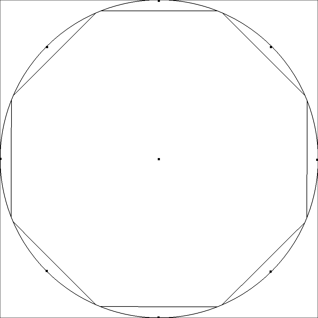
(c)	(d)

Figure 1: HVD for $k=1$ (a) and $k=2$ (b). HVD with all unbounded cells (c), and pencil of parallel bisectors intersecting at $\partial\mathbb{B}_{d}$ (d).

4.2 $k$-HVDs from power diagrams

Consider all subsets of size $k$, $\mathcal{P}_{k}={\mathcal{P}\choose k}=\{\mathcal{K}_{1},...,\mathcal{K}_{N}\}$ with $N={n\choose k}$. Those subset generators partition the space into non-empty $k$-order Voronoi cells:

$$\mathrm{Vor}_{k}(\mathcal{K}_{i})=\{x:\forall q\in\mathcal{K}_{i},\forall r\in\mathcal{P}\backslash\mathcal{K}_{i},\ D(x,q)\leq D(x,r)\}.$$

Observe that $x\in\mathrm{Vor}_{k}(\mathcal{K}_{i})$ iff $\sum_{p\in\mathcal{K}_{i}}D(x,p)\leq\sum_{p^{\prime}\in\mathcal{K}_{j}}D(x,p^{\prime})$. In Klein model with $D=d^{K}$, we define the function $\sigma_{\mathcal{K}_{i}}(x)=\sum_{x\in\mathcal{K}_{i}}\frac{1-{\langle x,p_{i}\rangle}}{\sqrt{1-{\langle p_{i},p_{i}\rangle}}}$, and $x\in\mathrm{Vor}_{k}(\mathcal{K}_{i})\Leftrightarrow h_{\mathcal{K}_{i}}(x)\leq h_{\mathcal{K}_{j}}(x)\ \forall j\not=i$. By identifying those hyperplane equations with the generic power diagram hyperplane $h(x):y=-2{\langle x,c\rangle}-w+{\langle c,c\rangle}$ for a ball centered at $c$ and radius $r^{2}=w$ ($r$ may be imaginary when $w<0$), we transform each $k$-subset $\mathcal{K}_{i}$ in Klein model into a weighted point (or ball) $\mathrm{ball}(c_{i},w_{i})$: $c_{i}=\sum_{p\in\mathcal{K}_{i}}\frac{p}{2\sqrt{1-{\langle p,p\rangle}}}$ and $w_{i}={\langle c_{i},c_{i}\rangle}-\sum_{p\in\mathcal{K}_{i}}\frac{1}{\sqrt{1-{\langle p,p\rangle}}}$. This method is only practical if when we consider all subsets $\mathcal{K}_{i}$ that yields non-empty cells, otherwise we have $N={n\choose k}$ too many balls to be tractable!

5 HVDs from the hyperboloid model

Consider the symmetric bilinear form $L=\mathrm{diag}(-1,1,...,1)$ in Minkowski space $\mathbb{R}^{1,d}$: ${\langle p,q\rangle}_{L}=p^{\top}Lq=-p^{(0)}q^{(0)}+\sum_{i=1}^{d}p^{(i)}q^{(i)}$. The hyperboloid model is defined on the upper sheet domain $\mathbb{L}^{+}=\{{\langle x,x\rangle}_{\mathrm{L}}=-1,\ x_{0}>0\}$ (interpreted as a sphere ${\langle x,x\rangle}_{\mathrm{L}}=R^{2}$ of imaginary radius $R=i$). For $x\in\mathbb{R}^{d}$, we denote $x^{L}$ its point obtained by vertically rising $(\cdot,x)$ on $\mathbb{L}^{+}$: $x^{L}=(\sqrt{1+{\langle x,x\rangle}},x)$, called Weierstrass coordinates. The hyperbolic distance is expressed by $D^{L}(p^{L},q^{L})=\mathrm{arccosh}(-{\langle p^{L},q^{L}\rangle}_{\mathrm{L}})$ and is equivalent to $d^{L}(p^{L},q^{L})=-{\langle p^{L},q^{L}\rangle}_{\mathrm{L}}$. For two points $p^{L}$ and $q^{L}$ on $\mathbb{L}^{+}$, the bisector equation is ${\langle x^{L},p^{L}-q^{L}\rangle}_{\mathrm{L}}=0$. The bisector is an hyperbola of equation $\left(\sqrt{1+{\langle p,p\rangle}}-\sqrt{1+{\langle q,q\rangle}}\right)\sqrt{1+{\langle x,x\rangle}}+{\langle q-p,x\rangle}=0,x\in\mathbb{R}^{d}\ (*)$. This hyperbola bisector is contained in a hyperplane $H(p,q)$ of $\mathbb{R}^{d+1}$ passing through the origin $O$: $H(p,q):(\sqrt{1+{\langle p,p\rangle}}-\sqrt{1+{\langle q,q\rangle}})x_{0}+{\langle q-p,x\rangle}=0$. The Klein disk model is obtained from $\mathbb{L}^{+}$ by a central projection $\pi$ from the origin to the hyperplane $H_{1}:x_{0}=1$: $\pi\left[\begin{array}[]{c}x_{0}\cr x\end{array}\right]=\left[\begin{array}[]{c}1\cr x^{\prime}=\frac{x}{x_{0}}=\frac{x}{\sqrt{1+{\langle x,x\rangle}}}\end{array}\right]$. The disk center touches the apex of $\mathbb{L}^{+}$. Let $a_{p,q}=\sqrt{1+{\langle p,p\rangle}}-\sqrt{1+{\langle q,q\rangle}}$. Multiplying $(*)$ by $\frac{1}{\sqrt{1+{\langle x,x\rangle}}}$, we have the bisector written as ${\langle q-p,x^{\prime}\rangle}+a_{p,q}=0$, an affine bisector in $x^{\prime}$.

Now consider $\pi_{c,l}$ the generic central projection of $\mathbb{L}^{+}$ from $C=(c,0)$ to the hyperplane $H_{l}:x_{0}=l$ so that $\pi=\pi_{0,1}$. We have $\pi_{c}\left[\begin{array}[]{c}\sqrt{1+{\langle x,x\rangle}}\cr x\end{array}\right]=\left[\begin{array}[]{c}l\cr x_{c,l}=\frac{l-c}{\sqrt{1+{\langle x,x\rangle}}-c}x\end{array}\right],c\not=1$. Choosing $c=0$ and $0<l\leq 1$ yields the same construction procedure but the clipping of the equivalent power diagram [1] need to be done on a disk of size $l$ since $\|x_{c,l}\|=\|\frac{l}{\sqrt{1+{\langle x,x\rangle}}}x\|\leq l$, $\forall x\in\mathbb{R}^{d}$.

Note that clipping may destroy bounded cells of the affine diagram as illustrated in Figure 2. Thus a remaining open question is to report an optimal output-sensitive construction of the $k$-order HVDs.

A video illustrating the hyperbolic Voronoi diagrams using the five common models of hyperbolic geometry is available online [4].

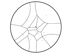
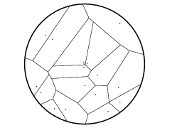
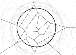
(a)	(b)	(c)

Figure 2: The hyperbolic Voronoi diagram in conformal Poincaré disk (a) is obtained by a radial scaling transformation of the HVD in non-conformal Klein disk (b) that is itself built as an equivalently clipped power diagram (c). Observed that some bounded cells of the power diagram are cut by the boundary cutting circle.

References

- [1] Frank Nielsen and Richard Nock. Hyperbolic Voronoi diagrams made easy. In B. O. Apduhan et al., editor, International Conference on Computational Science and Its Applications, pages 74–80. IEEE, 2010.
- [2] Frank Nielsen and Richard Nock. The hyperbolic Voronoi diagram in arbitrary dimension. arXiv preprint arXiv:1210.8234, 2012.
- [3] Frank Nielsen and Richard Nock. Visualizing hyperbolic Voronoi diagrams. In Symposium on Computational Geometry. ACM, 2014. http://www.youtube.com/watch?v=i9IUzNxeH4o.
- [4] Frank Nielsen and Richard Nock. Visualizing hyperbolic Voronoi diagrams. In Proceedings of the Thirtieth Annual Symposium on Computational Geometry, SOCG’14, pages 90:90–90:91, New York, NY, USA, 2014. ACM.