Reconnection Properties of Large-Scale Current Sheets During
Coronal Mass Ejection Eruptions

Abstract

We present a detailed analysis of the properties of magnetic reconnection at large-scale current sheets in a high cadence version of the Lynch & Edmondson (2013) 2.5D MHD simulation of sympathetic magnetic breakout eruptions from a pseudostreamer source region. We examine the resistive tearing and breakup of the three main current sheets into chains of X- and O-type null points and follow the dynamics of magnetic island growth, their merging, transit, and ejection with the reconnection exhaust. For each current sheet, we quantify the evolution of the length-to-width aspect ratio (up to $\sim$100:1), Lundquist number ($\sim$10³), and reconnection rate (inflow-to-outflow ratios reaching $\sim$0.40). We examine the statistical and spectral properties of the fluctuations in the current sheets resulting from the plasmoid instability, including the distribution of magnetic island area, mass, and flux content. We show that the temporal evolution of the spectral index of the reconnection-generated magnetic energy density fluctuations appear to reflect global properties of the current sheet evolution. Our results are in excellent agreement with recent, high resolution reconnection-in-a-box simulations even though our current sheets’ formation, growth, and dynamics are intrinsically coupled to the global evolution of sequential sympathetic CME eruptions.

1 Introduction

The magnetic reconnection rate from the Sweet-Parker reconnection model (Sweet, 1958; Parker, 1963) for elongated current sheets is generally too “slow” to account for the observed rapid flux transfer in solar flares. The solar corona is extremely conductive so the magnetic Reynolds number (the Lundquist number) is of the order of $S=4\pi\sigma V_{A}L/c^{2}\sim 10^{10-12}$ where $V_{A}$ is the Alfven speed, $L$ is a characteristic global length scale, $\sigma$ is the plasma conductivity, and $c$ is the speed of light. The scaling of the Sweet-Parker reconnection inflow velocity $V_{in}$ to the reconnection outflow velocity (taken as $V_{A}$) goes as $V_{in}/V_{A}\sim S^{-1/2}$, yielding theoretical inflow speeds of $V_{in}\lesssim 10^{-5-6}V_{A}$. The Petschek (1964) reconnection model is able to obtain the much greater inflow speeds needed for “fast” reconnection, e.g. $V_{in}\sim 0.10V_{A}$, but requires a much shorter current sheet (essentially a single X-point) and a very localized enhancement of the magnetic resistivity (equivalently, a very localized depletion of the plasma conductivity). In collisionless reconnection models, the scales of kinetic dissipation effects are sufficiently small ($\sim$$10^{2}$ cm) that these models are also able to produce fast, Petschek-like reconnection scenarios. Given that the highest resolution observations of current sheets in the corona are still macroscopic in scale (i.e., $10^{6-7}$ cm), it is not clear if or how the microscopic – and presently unobservable – Petschek or Petschek-like reconnection processes relate to these large-scale observations. Therefore, a tremendous body of work on detailed reconnection studies, both analytical and numerical, has been dedicated to attempting to resolve this situation (e.g., see Cassak & Drake, 2013, and references therein). Significant progress has been made in understanding the physical processes that effectively “speed up” the reconnection rates associated with large-scale current sheets.

One of the ways to speed up the reconnection is the onset and development of instabilities that result in current sheet tearing, breakup, and the formation of magnetic island plasmoids (Furth et al., 1963; Forbes & Priest, 1983; Biskamp, 1996). The onset of the resistive tearing mode has been characterized by the fastest growing wavelengths associated with linearized perturbation analysis and advances in numerical modeling have enabled simulations of the highly nonlinear time-dependent evolution of the plasmoid instability (e.g., Forbes & Malherbe, 1991; Karpen et al., 1998, 2012; Loureiro et al., 2007; Lin et al., 2009; Samtaney et al., 2009; Bhattacharjee et al., 2009; Huang & Bhattacharjee, 2010; Ni et al., 2010, and references therein).

An alternative way to speed up reconnection is to make the current sheet thin enough that traditional (resistive) MHD formalism breaks down. If the current sheet dissipation region becomes smaller than the ion skin depth then the system enters a collisionless regime which can generate reconnection rates orders of magnitude faster than Sweet-Parker. Modeling this regime is accomplished by either including the generalized Ohm’s law (“Hall MHD”) or by going to a hybrid (electron fluid, ion particle) or fully kinetic particle treatment; see, e.g., the results of the GEM reconnection challenge (Birn et al., 2001; Birn & Hesse, 2001; Hesse et al., 2001; Kuznetsova et al., 2001; Ma & Bhattacharjee, 2001; Otto, 2001; Pritchett, 2001; Shay et al., 2001).

In fact, these two approaches to speed up the reconnection – current sheet tearing and plasmoid formation in traditional MHD and the inclusion of more physics and particle effects in the numerical modeling (Hall MHD, hybrid, particle codes) – are not mutually exclusive. The break-up of large-scale current sheets into chains of magnetic islands appears to be a robust and universal feature in all of the different types of 2D reconnection modeling (e.g., Drake et al., 2006b; Daughton et al., 2006, 2009; Cassak et al., 2009b). The discussion by Edmondson et al. (2010) provides some important physical insight into why the plasmoid formation appears to be such a robust, universal process.

The physical properties that govern the reconnection dynamics in a current sheet are determined by the global system. The geometry of the current sheet, its length and width, are related to the global scale of the magnetic configuration and the scale at which the frozen-in flux condition breaks (the diffusion scale), respectively. In MHD simulations, the diffusion scale is set by the resistivity model which, at its smallest value, is essentially the scale of the numerical grid. In simulations that include particle effects, the diffusion scale is given by the ion skin depth or gyroradius. The inflow and outflow velocities transporting magnetic flux into the current sheet and reconnected flux out in the exhaust are likewise determined by the global system. The inflow velocities are typically boundary conditions in dedicated reconnection simulations or, as in our case here, determined by the global dynamics of the magnetic field, and the outflow velocities are of the order of the Alfven speed. Since the global system has determined all the key parameters governing the reconnecting current sheet, the additional constraints the system must operate under, such as the conservation of mass and magnetic flux, means the system is actually over-determined. The break-up of the current sheet and the formation of magnetic islands resolves this over-determination by introducing new scales into the system that allow both the conservation laws and the global constraints on the current sheet reconnection properties to be met simultaneously.

The purpose of this paper is to examine, in detail, the properties and evolution of magnetic reconnection and the magnetic island plasmoids generated in the current sheets that arise in the sympathetic eruption scenario of Lynch & Edmondson (2013), hereafter abbreviated as L&E13. The paper is structured as follows. In Section 2, we briefly discuss the MHD code and review the L&E13 simulation results that self-consistently create the three large-scale current sheets during two sequential CME eruptions. In Section 3, we compare the global properties and evolution of the current sheets in terms of their Lundquist number, inflow and outflow properties, and reconnected magnetic flux. In Section 4, we present distribution functions of the island area, mass and flux content, and examine the spectral properties of the magnetic fluctuations in the current sheets. In Section 5, we discuss the implications of our results and the direction of future work.

2 Numerical Simulation Methods and Summary of Previous Results

2.1 ARMS: Adaptively Refined MHD Solver

The Adaptively Refined MHD Solver (ARMS; DeVore & Antiochos, 2008) calculates solutions to the 3D nonlinear, time-dependent MHD equations using a finite-volume flux-corrected transport numerical scheme (DeVore, 1991). ARMS is fully integrated with the adaptive mesh toolkit PARAMESH (MacNeice et al., 2000) to handle solution-adaptive grid refinement and support efficient multi-processor parallelization. ARMS has been used to perform a wide variety of numerical simulations of dynamic phenomena in the solar atmosphere, including 3D magnetic breakout CME initiation (DeVore & Antiochos, 2008; Lynch et al., 2008), the eruption of coronal jets (Pariat et al., 2009, 2010), the interaction between closed and open fields at streamer belt boundaries (Edmondson et al., 2009) and during CME eruptions (Masson et al., 2013), and the detailed examination of current sheet formation, magnetic reconnection, and magnetic island creation (Edmondson et al., 2010; Karpen et al., 2012; Guidoni et al., 2016).

For the simulation discussed herein, we use ARMS to solve the ideal MHD equations in Cartesian coordinates,

$$\frac{\partial\rho}{\partial t}+\nabla\cdot\left(\rho\mathbf{V}\right)=0,$$ (1)

$$\frac{\partial\left(\rho\mathbf{V}\right)}{\partial t}+\nabla\cdot\left(\rho\mathbf{V}\mathbf{V}\right)+\nabla P=\frac{1}{4\pi}\left(\nabla\times\mathbf{B}\right)\times\mathbf{B},$$ (2)

$$\frac{\partial T}{\partial t}+\nabla\cdot\left(T\mathbf{V}\right)+\left(\gamma-1\right)T\left(\nabla\cdot\mathbf{V}\right)=0,$$ (3)

$$\frac{\partial\mathbf{B}}{\partial t}=\nabla\times\left(\mathbf{V}\times\mathbf{B}\right).$$ (4)

The variables retain their usual meaning: mass density $\rho$, velocity $\mathbf{V}$, magnetic field $\mathbf{B}$, and we have written the energy equation in terms of the plasma temperature $T$. The ratio of specific heats is $\gamma=5/3$ and the ideal gas law $P=2(\rho/m_{p})k_{B}T$ closes the system. Additionally, while there is no explicit magnetic resistivity in the equations of ideal MHD, necessary and stabilizing numerical diffusion terms introduce an effective resistivity on very small spatial scales, i.e. the size of the grid. In this way, magnetic reconnection can occur when sharp magnetic gradients of field component reversals and their associated current sheet features have been compressed to the local grid resolution scale.

The full computational domain is $x\in[-5,5]$, $y\in[1,21]$ in units of the characteristic length scale $L_{0}=10^{9}$ cm. There are six total levels of static grid refinement that vary in the $y$ direction. For the $y\in[1,11]$ region analyzed herein: $1\leq y\leq 7.094$ is level six, $7.094<y\leq 9.750$ is level five, and $9.750<y\leq 11$ is level four. The highest refinement region corresponds to an effective $1024\times 1024$ resolution and we have interpolated the lower refinement regions to this resolution. The current sheets that we will examine remain entirely in the level six portion of the domain.

The initial magnetic field configuration is constructed from the magnetic vector potential of a series of line dipoles to create the pseudostreamer arcades embedded in a uniform vertical background field (see also Edmondson et al., 2010). The background field strength is $B_{0}=5$ G whereas the line dipoles yield field strengths in the pseudostreamer arcades of $\sim$35 G. The initial uniform mass density $\rho_{0}=10^{-16}$ gm cm^-3 and pressure $P_{0}=0.01$ dyn cm^-2 result in a global plasma beta of $\beta_{0}\sim 0.01$ and global Alfven speed $V_{A0}\sim 1400$ km s^-1.

The system is energized with shear flows at the lower boundary parallel to the pseudostreamer arcade polarity inversion lines that are smoothly ramped up, remain uniform for $\sim$1000 s, and then are smoothly ramped back down to zero (see Figure 1 of L&E13, ). In order for reconnection to proceed in our system, the initial symmetry is broken by ramping down the shearing flows in the left psuedostreamer arcade first and continuing the uniform shearing in the right arcade for an additional 150 s. This has the effect of distorting the pseudostreamer X-point by the separation of the inner and outer spine lines as in the Syrovatskii (1971, 1978a, 1978b, 1981) scenario and forming the initial overlying “magnetic breakout” current sheet. The development of this current sheet for $t\gtrsim 1250$ s, as well as the subsequent sympathetic CMEs that each form their own eruptive flare current sheets, is entirely due to the global response of the system to the accumulated free magnetic energy supplied by the shearing flows.

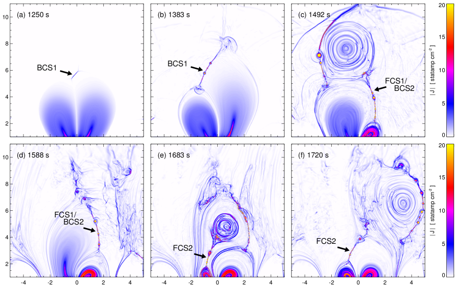
Figure 1: Summary plot of the current density magnitude $|J|$ illustrating the sympathetic magnetic breakout eruption scenario. Panels (a) and (b) show the breakout phase and BCS1. Panels (c) and (d) show the first eruption, FCS1/BCS2, and the transition of FCS1/BCS2 into the breakout phase for the second eruption. Panels (e) and (f) show the second eruption and FCS2. An animation of this figure is available as an electronic supplement to the online version (FIGURE1_jm.mp4).

2.2 Sympathetic Breakout Eruption Scenario

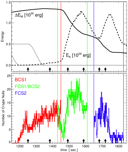
Figure 2: Upper panel: global magnetic free energy ($\Delta E_{M}$) and kinetic energy ($E_{K}$) evolution. Lower panel: number of O-type null points (magnetic islands) in each current sheet (BCS1 red; FCS1 green; FCS2 blue). The black arrows correspond to the times shown in the six panels of Figure 1.

L&E13 discussed the global evolution and interaction of the pseudostreamer and background flux systems during the sympathetic magnetic breakout eruption process. This was largely an extension of the idea presented by Török et al. (2011) who showed that quasi-stable flux ropes anchored in the arcades of a pseudostreamer could be made to erupt in sequence if a sufficiently large perturbation was introduced. Török et al. (2011) highlighted the evolution of various current sheets that form in response to this perturbation (which in their numerical simulation was the eruption of a third flux rope in the vicinity of the pseudostreamer). Those authors also noted the similarities of the system’s magnetic topology to that required for the magnetic breakout CME initiation model (Antiochos et al., 1999; MacNeice et al., 2004; DeVore & Antiochos, 2008; Karpen et al., 2012).

L&E13 confirmed that the sympathetic eruption sequence could, in fact, be initiated via magnetic breakout and showed that each eruption resulted in a fast $\gtrsim 1500$ km s^-1 flux rope CME that was formed by the flare reconnection above the polarity inversion line of one of the pseudostreamer arcades. The simulation resolution was sufficiently high such that we were able to model the detailed structure and evolution of the current sheet during the onset and development of the plasmoid instability. We presented those results qualitatively in the context of the adaptive mesh refinement runs by Karpen et al. (2012) which showed that the onset of “fast” reconnection associated with the current sheet tearing and ubiquitous magnetic island formation was directly responsible for, and essentially defined, the acceleration phase of the CME eruption.

Figure 1 plots six frames of current density magnitude $|J|$ during the sympathetic magnetic breakout eruption scenario. Panels 1(a), (b) show the period of overlying breakout reconnection that evolves (relatively) slowly and acts to remove restraining flux from above the sheared field core which will eventually become the center of the first erupting flux rope-like structure. We have labeled this first breakout current sheet BCS1. Panel 1(c) shows the eruption of the first CME from the right arcade of the pseudostreamer. The runaway expansion from the expansion-breakout reconnection positive feedback enables the formation of the second, essentially vertical current sheet underneath the rising sheared field core, just as in the standard CSHKP eruptive flare picture (Carmichael, 1964; Sturrock, 1966; Hirayama, 1974; Kopp & Pneuman, 1976). Here we label the first flare current sheet FCS1/BCS2. Panel 1(d) shows the system’s further evolution where the continued reconnection at FCS1/BCS2 acts as the overlying breakout reconnection for the left pseudostreamer arcade, facilitating a second runaway expansion-breakout reconnection feedback loop. Finally, in panels 1(e), (f) we show the second CME with its eruptive flare current sheet labeled FCS2. The accompanying online animation FIGURE1_jm.mp4 shows the complete temporal evolution of the sympathetic eruptions.

In order to analyze the fine-scale structure and dynamics of the current sheets, we re-ran the L&E13 simulation with a factor of 10 higher cadence for the output data files. The L&E13 simulation was run on the UCB SSL cluster “Shodan” (Intel Xeon Harpertown architecture, Open MPI 1.4.5 and Intel 12.1 compilers) while the present simulation was performed on NASA NCCS “Discover” cluster (Intel Xeon Sandy Bridge architecture, Open MPI 1.7.2 and Portland Group 13.6 compilers). Despite small, quantitative numerical differences accumulating over hundreds of thousands of computational time steps, the sympathetic eruptive flare and CME onset times agree to within $\sim$4% between the two simulations (i.e., $\Delta T_{\rm CME1}/T_{\rm CME1}=50/1470=0.034$ and $\Delta T_{\rm CME2}/T_{\rm CME2}=70/1670=0.042$).

The top panel of Figure 2 shows the global magnetic and kinetic energy evolution in our system once the symmetry has been broken by the energization flows applied to the lower boundary. The solid line is the total free magnetic energy $\Delta E_{M}(t)=E_{M}(t)-E_{M}(0)$ where the initial magnetic energy of the potential field at $t=0$ is $E_{M}(0)=9.96\times 10^{29}$ erg. The dashed line is the total kinetic energy $E_{K}(t)$. The gray lines indicate the temporal duration of the boundary shearing flows: by 1150 s the left arcade driving flow is half of the way through its ramp down, and the right arcade driving flows begin to be ramped down at 1250 s. The kinetic energy slowly rises during the period of breakout reconnection to $\sim$10²⁸ erg before the onset of flare reconnection in FCS1/BCS2 starts the impulsive acceleration of the first CME – signaled by the rapid rise of $E_{K}$ to a peak of $1.3\times 10^{29}$ erg and the rapid decrease in free magnetic energy of $7\times 10^{29}$ erg. The rate of magnetic energy decrease slows as FCS1/BCS2 transitions from CME1’s eruptive flare reconnection to the breakout reconnection above the left arcade. The onset of FCS2 reconnection signals the second CME’s eruption and $E_{K}$ peak of $1.2\times 10^{29}$ erg during a free magnetic energy drop of $\sim 3\times 10^{29}$ erg. The vertical lines indicate the temporal window in the simulation in which we will examine each of the large-scale current sheets in detail: BCS1 red, FCS1/BCS2 green, and FCS2 blue. The black arrows correspond to the six panels in Figure 1.

3 Comparison of the Breakout and Eruptive Flare Current Sheets

The onset of reconnection in our large-scale current sheets and the development of the tearing mode plasmoid instability can be seen in the bottom panel of Figure 2 where we have plotted the number of magnetic O-type null points (magnetic islands) present in each of our three current sheets as a function of time. The procedure used to identify the X-type and O-type null points is described in the Appendix of Karpen et al. (2012). For each simulation output file, the spatial position, type, and degree of every magnetic null is recorded and here we have plotted only the number of O-type nulls present in BCS1 (red), FCS1/BCS2 (green), and FCS2 (blue). There is an approximate correspondence between the global kinetic energy $E_{K}(t)$ and the number of magnetic islands – most visible in the rapid rise phases of $E_{K}$ associated with the main CME acceleration phase of the eruptions.

As BCS1 is stretched out and becomes unstable to tearing, the number of magnetic islands grows from zero to $\sim$10 by 1250 s. By this point the islands are being continually ejected into and by the reconnection outflow exhaust and the resistive tearing of the sheet has saturated to somewhat of a quasi “steady-state.” Continued reconnection drives new island formation and these, in turn, are ejected from the sheet. So from $1250\lesssim t\lesssim 1450$ s the rate of new island creation slightly outpaces the rate of old island ejection and we see fluctuations around an essentially linear trend from $\sim$5 to $\sim$12 islands present in BCS1 as it grows (and fluctuates) in length and is pushed higher into the simulation domain by the expanding arcade system from below. BCS1 starts with an initial X-type null point and develops into a current sheet via the separation of the spine lines (Syrovatskii, 1981; Antiochos et al., 2002; Edmondson et al., 2010) due to the expansion of the right pseudostreamer arcade.

Figure 3 shows the zoomed-in view of BCS1 and its online animation (FIGURE3_bcs1.mp4) shows the temporal evolution. Panel (a) is the electric current density $|J|$, panel (b) is the plasma number density ($\rho/m_{p})$, and panels (c) and (d) plot the plane-of-the-sky components of the plasma velocity normalized to the global Alfven speed, $V_{y^{\prime}}/V_{A0}$ and $V_{x^{\prime}}/V_{A0}$. Here, the rectangular current-sheet centered coordinate frame ($x^{\prime},y^{\prime}$) corresponds to a standard translation and rotation from the initial simulation reference frame. The ($x^{\prime},y^{\prime}$) frame locations and orientations were initially estimated by visual inspection and then prescribed as analytic functions of time in order to smoothly track the evolution of the current sheets throughout the simulation domain (see Appendix A for details). The resulting frame orientations are such that the plasma velocity $y^{\prime}$-component in panel (c) of Figure 3 is approximately aligned with the inflow into the current sheet and the $x^{\prime}$-component in panel (d) is approximately aligned with the reconnection outflow.

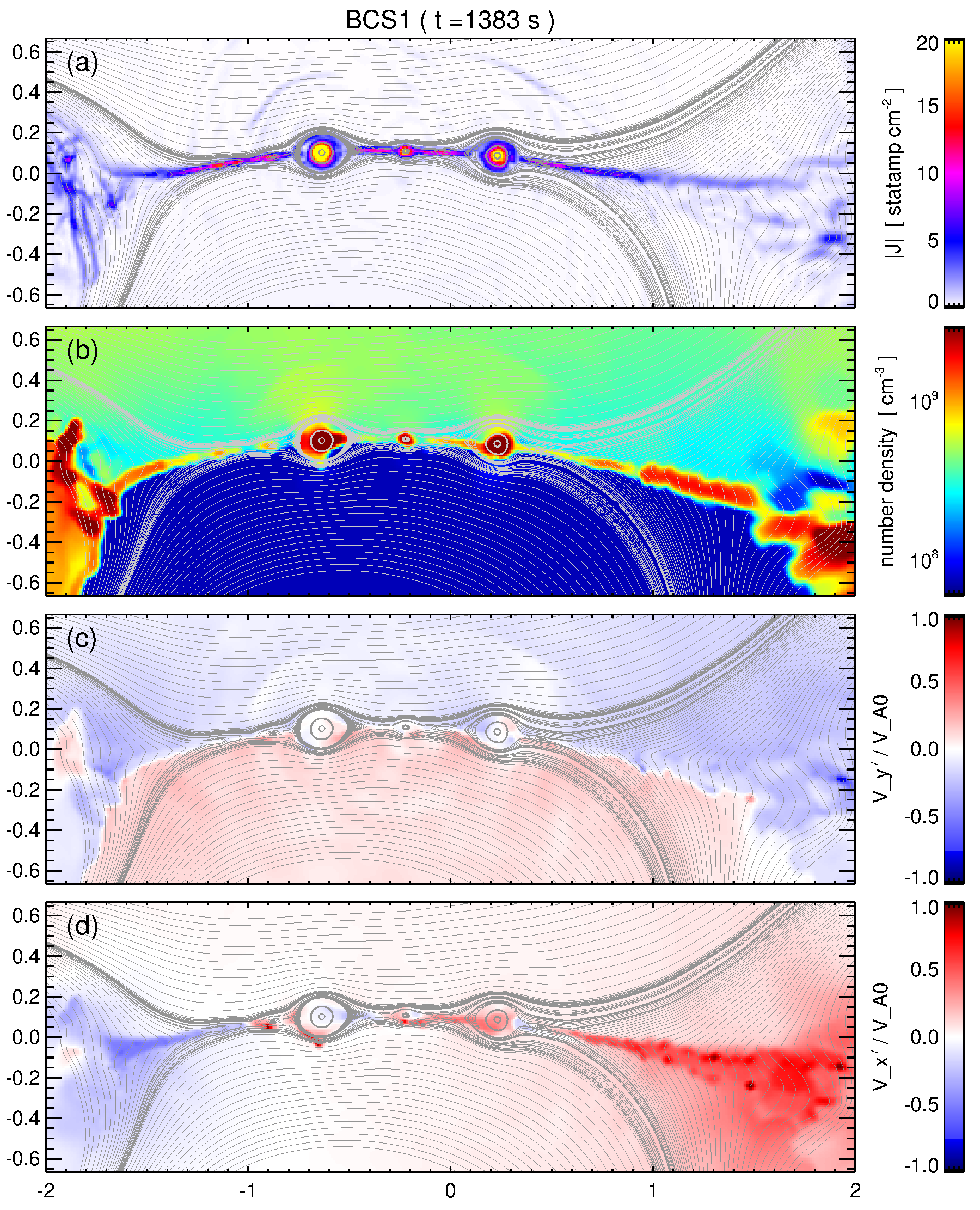
Figure 3: Plasma properties of the BCS1 current sheet at $t=1383$ s: (a) plots current density magnitude $|J|$, (b) number density $\rho/m_{p}$, (c) approximate reconnection inflow $V_{y^{\prime}}/V_{A0}$, and (d) approximate reconnection outflow $V_{x^{\prime}}/V_{A0}$. Representative magnetic field lines are also plotted in each panel illustrating the CS structure and island formation. An animation of this figure is available as an electronic supplement to the online version (FIGURE3_bcs1.mp4).

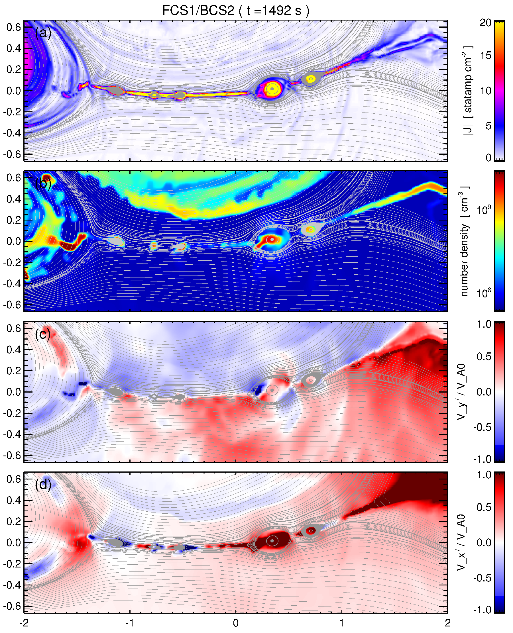
Figure 4: Plasma properties and field configuration of FCS1/BCS2 at $t=1492$ s in the same format as Figure 3. An animation of this figure is available as an electronic supplement to the online version (FIGURE4_fcs1.mp4).

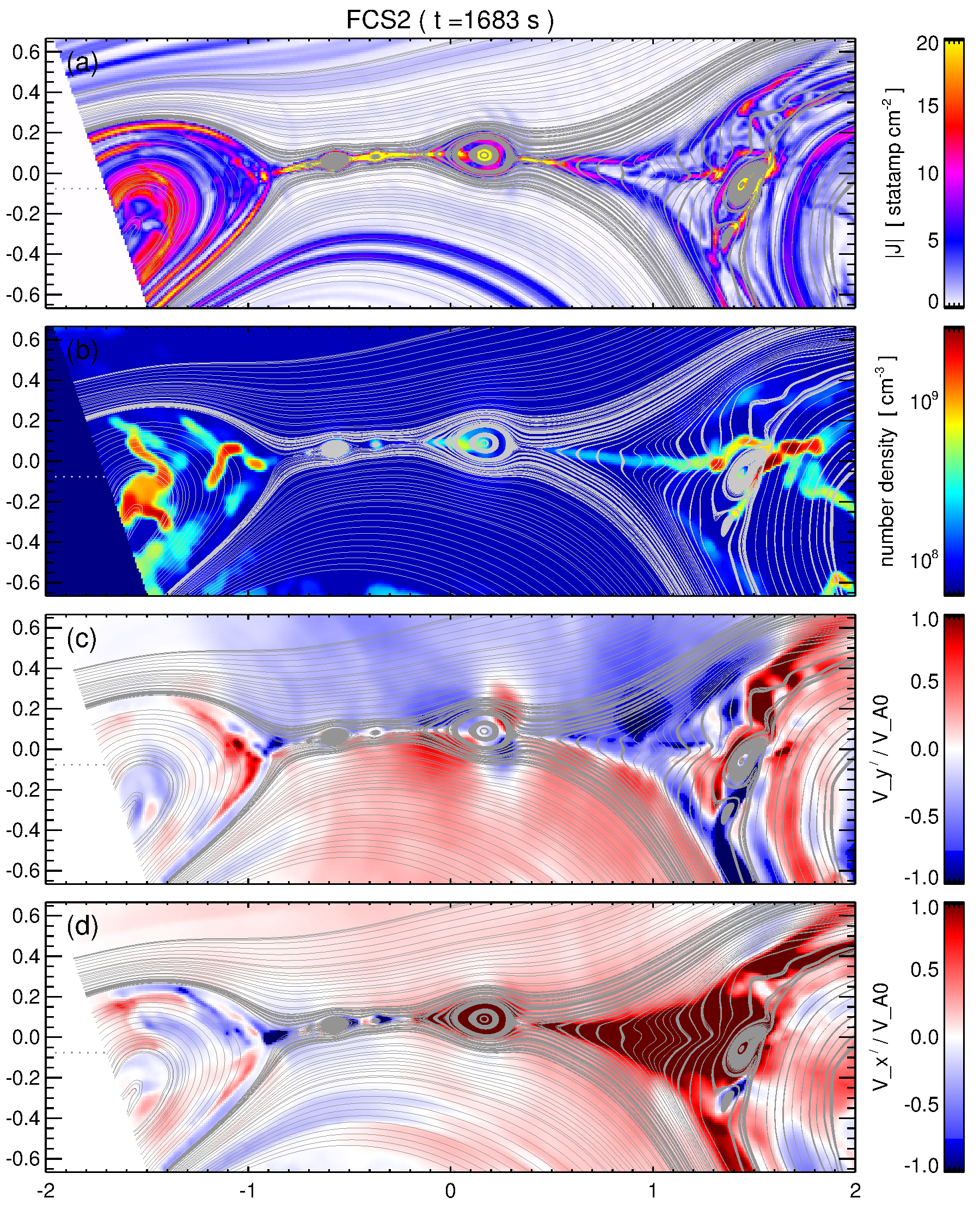
Figure 5: Plasma properties and field configuration of FCS2 at $t=1683$ s in the same format as Figure 3. An animation of this figure is available as an electronic supplement to the online version (FIGURE5_fcs1.mp4).

The evolution of FCS1/BCS2 and FCS2 start with a different onset scenario. For the eruptive flare current sheets, each of the pseudostreamer arcades has a significant shear component that accumulates over the course of the imposed boundary flows, thus developing oppositely directed field components (in the plane of the sky) and an associated vertical current sheet above the polarity inversion line. This is a universal feature of all sheared arcade models (Aulanier et al., 2002, 2006; Welsch et al., 2005) that is also present in sigmoidal field structures (Sterling, 2001; Canfield et al., 2007; Green & Kliem, 2009; Savcheva et al., 2012a), flux emergence simulations (Gibson & Fan, 2006; Manchester et al., 2004; Manchester, 2008), and analytic and numerical treatments of flux rope models (Forbes & Isenberg, 1991; Titov & Démoulin, 1999; Isenberg & Forbes, 2007; Lin et al., 2009; Savcheva et al., 2012b).

Figures 4, 5 show the zoomed-in views of FCS1/BCS2 and FCS2, respectively, in the same format as Figure 3. Their corresponding online animations, FIGURE4_fcs1.mp4 and FIGURE5_fcs2.mp4, show their respective temporal evolutions. Again, Appendix A describes the bulk motion of the ($x^{\prime},y^{\prime}$) coordinate frames for each of the eruptive flare current sheets periods.

The number of magnetic islands in FCS1/BCS2 is shown to start moderately high ($\sim$10) and shrinks down to one by $t\sim 1460$ s before rapidly increasing to the 15–20 range. For $t\lesssim 1460$ s the eruptive flare reconnection has not yet started in earnest. FCS1/BCS2 exists with fluctuations in the neutral sheet corresponding to multiple X- and O-type nulls, but there is virtually no reconnection inflow per se. It takes the runaway arcade expansion to disrupt the force balance sufficiently to thin the current sheet sufficiently that numerical resistivity allows the reconnection to proceed. Unlike the breakout reconnection, there is a significant drop in magnetic energy so the FCS1/BCS2 outflow exceeds the global Alfvén speed ($|V_{x^{\prime}}|\gtrsim 1.5V_{A0}$) and processes a significant amount of flux before the CME eruption stretches out FCS1/BCS2 to lengths where the tearing mode is in full effect ($t\gtrsim 1490$ s).

The second eruptive flare sheet FCS2 has the same overall dynamics and evolution as FCS1/BCS2 for approximately the first half of its 180 s duration. Again we see the initial sheared-arcade vertical current sheet with some islands but very little reconnection inflow until $\sim$1670 s when the CS outflow exceeds the global Alfvén speed during the impulsive phase of the eruption. FCS2 then rapidly grows beneath the erupting flux rope, leveling off in the $\sim$10 island range. Once $t\gtrsim 1740$ s most of the remaining free energy has been released and the pseudostreamer arcades are able to relax towards a state much closer to the initial potential field configuration. The FCS2 reconnection dissipates the current density enhancement and the CS length shrinks, i.e. the spine field lines are moving closer together in an attempt to restore the original X-point null topology. The reconnection becomes much smoother during this relaxation phase and this can be seen in the number of magnetic islands dwindling to the one or two level.

3.1 Dimensionless Analysis: Evolution of the Global Lundquist Number

We define the Lundquist number in the usual fashion by comparing the annihilation timescale with the communication timescale along the current sheet, $S\equiv\tau_{\eta}/\tau_{A}$, where $\tau_{\eta}=L^{2}/{\eta}$ and $\tau_{A}={L}/V_{A}$. $L$ is the half-length of the current sheet, $\eta$ is the diffusion term within the current sheet and $V_{A}$ the upstream Alfvén speed. Thus,

$$S\equiv\frac{\tau_{\eta}}{\tau_{A}}=\left(\frac{L^{2}}{\eta}\right)\left(\frac{V_{A}}{L}\right)=\frac{L\ V_{A}}{\eta}.$$ (5)

In our simulation, the magnetic resistivity is purely numerical and may be estimated by balancing the inflow speed $V_{in}$ of magnetic flux into the current sheet against the resistive annihilation across the current sheet,

$$\tau_{in}=\tau_{\eta}\ \Longrightarrow\ \frac{\delta}{V_{in}}=\frac{\delta^{2}}{\tilde{\eta}}\ \Longrightarrow\ \tilde{\eta}=\delta\ V_{in},$$ (6)

where $\delta$ is the half-thickness of the current sheet. Here we take our current sheet thickness to be the width of two computational cells at the highest grid resolution (as in Karpen et al., 2012), obtaining $\delta=10L_{0}/1024=0.00977L_{0}=9.77\times 10^{6}$ cm. The numerical resistivity estimates are on the order of $10^{14}$ cm² s^-1 with mean values over the BCS1, BCS2/FCS1, and FCS2 durations of $\tilde{\eta}\sim 9.5\times 10^{13}$ cm² s^-1, $2.6\times 10^{14}$ cm² s^-1, and $2.9\times 10^{14}$ cm² s^-1, respectively. We also note this range is less than (i.e., compatible with) the estimate of the strict upper-limit of the numerical resistivity, $\tilde{\eta}_{\rm max}\equiv C\Delta x^{2}/\Delta t$, where $C$ is the Courant number, $\Delta x$ is the grid size ($\delta$) and $\Delta t$ is the size of the computational time step (DeVore 2014, private communication). Substituting our numerical resistivity estimate into the Lundquist number characterizing the current sheet yields $S=(LV_{A})/(\delta V_{in})$.

We construct sheet-averaged quantities in order to estimate an average, global Lundquist number as a function of simulation time,

$$\langle S(t)\rangle=\frac{L(t)}{\delta}\frac{V_{A0}}{\langle V_{in}\rangle}.$$ (7)

Here, $L(t)$ is the estimate of the half-length of the sheet, $V_{A0}$ is the global Alfven speed, and $\langle V_{in}\rangle$ represents the area average of the inflow velocities. Appendix B provides the complete mathematical description of CS geometries and Appendix C describes the method used to generate the sheet-averaged estimates from the simulation data.

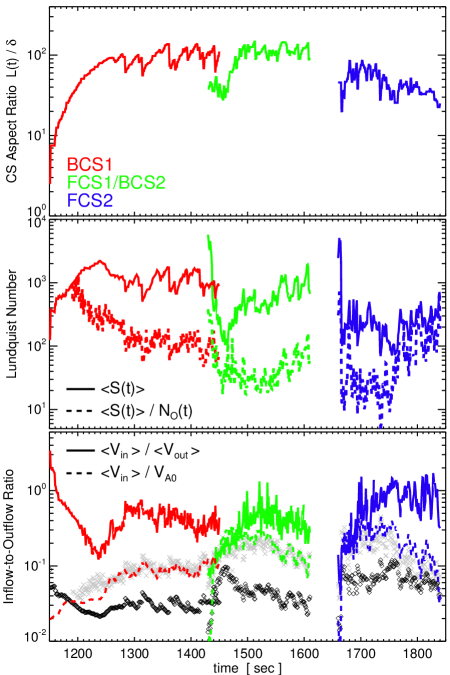
Figure 6: Top panel: The length-to-width aspect ratio $L(t)/\delta$ for each of the three current sheets (BCS1 red; FCS1/BCS2 green; FCS2 blue). Middle panel: The global CS-averaged Lundquist number ($\langle S\rangle$; solid) and the estimate of the local CS-averaged Lundquist number ($\langle S\rangle/N_{O}$; dashed). Bottom panel: The CS-averaged inflow-to-outflow ratio ($\langle V_{in}\rangle/\langle V_{out}\rangle$; solid), the inflow-to-global Alfvén speed ratio ($\langle V_{in}\rangle/V_{A0}$; dashed), the theoretical Sweet-Parker scaling ($S^{-1/2}$; black diamonds), and the plasmoid-modified Sweet-Parker scaling ($S^{-1/2}N_{O}^{1/2}$; gray crosses). See text for details.

The top panel of Figure 6 plots the time evolution of the average CS aspect ratio $L(t)/\delta$ for BCS1 (red), FCS1/BCS2 (green), and FCS2 (blue). The BCS1 aspect ratio clearly shows the rapid formation and elongation of the CS as the spine lines separate and a gradual leveling-off at $\sim$80:1 by $t\gtrsim 1250$ s. From this point onward the BCS1 aspect ratio fluctuates around this level, ranging from 60:1–100:1. The sharp decreases in length correspond to ejections of large plasmoids and typically the sheet lengthens again until the next large plasmoid ejection. The FCS1/BCS2 aspect ratio shows essentially the same large-scale evolution. Starting with the onset of flare reconnection ($t\sim 1460$ s), the FCS1/BCS2 aspect ratio grows from 30:1 to $\sim$100:1 before leveling-off. FCS2 on the other hand, while showing similar rapid growth starting from its flare reconnection onset ($t\sim 1670$ s), starts from a ratio of $\sim$20:1 but levels-off earlier at $\sim$60:1 before gradually shrinking back towards the $\sim$20:1 level over the course of $1750\lesssim t\lesssim 1840$ s.

The middle panel of Figure 6 plots the global CS-averaged Lundquist number $\langle S(t)\rangle$, given by Equation 7, as a function of time in each of the three sheets (BCS1 red; FCS1/BCS2 green; FCS2 blue). The behavior of $\langle S(t)\rangle$ shows a similar evolution to the CS aspect ratio. The BCS1 Lundquist number increases rapidly to $10^{3}$ through 1200 s during the elongation of the CS and then continues to increase more gradually until it reaches $2\times 10^{3}$ by 1250 s. The Lundquist number then fluctuates around approximately $10^{3}$ through the rest of the CS evolution. The FCS1/BCS2 current sheet has a comparable average Lundquist number of $\sim$800–1000 but transitions from higher values due to an initially near-zero inflow velocity. Once plasmoid-unstable reconnection has started, FCS1/BCS2 also fluctuates around this average. The average FCS2 $\langle S(t)\rangle$ is a bit lower, at $\sim$200–400 as the current sheet dissipates.

The middle panel of Figure 6 also plots $\langle S(t)\rangle/N_{O}(t)$ as dotted lines corresponding the global Lundquist number divided by the number of O-type magnetic null points, $N_{O}$, from Figure 2. This is an estimate of the CS-averaged local Lundquist number for the CS intervals between islands. Cassak et al. (2009b), Daughton et al. (2009), Uzdensky et al. (2010), and others have argued that during the non-linear phase of the instability these secondary sheets also reach the tearing threshold, go unstable, and start to generate islands. Our static computational grid imposes the minimum CS thickness of $\delta$ so we do not resolve the thinning of the secondary sheets in this simulation. Thus, in a statistical sense, the “steady state” number of magnetic islands, $N_{O}\sim 10$, and global $S\sim 10^{3}$ imply secondary sheets with $S_{local}\sim 10^{2}$.

The canonical critical Lundquist number is typically taken as $\sim$10⁴ (e.g., Biskamp, 1986; Samtaney et al., 2009; Huang & Bhattacharjee, 2010; Loureiro et al., 2012; Murphy et al., 2013, and references therein) but again, the plasmoid instability has been shown to develop over a wide range of values depending on the specific simulation details. Under steady-state driving (inflow) conditions, the Edmondson et al. (2010) MHD simulations were plasmoid unstable and comfortably in the nonlinear regime at $S\sim 1.2\times 10^{3}$, consistent with the Ni et al. (2010) and Shen et al. (2011) results. Here, our global Lundquist number is similar to Edmondson et al. (2010) but our inflow-to-outflow ratio is higher and our magnetic island plasmoids appear to cover a much greater dynamic range in size (discussed further in Section 4.1).

The bottom panel of Figure 6 shows two different measures of the CS-averaged inflow-to-outflow ratio. The solid line shows $\langle V_{in}\rangle/\langle V_{out}\rangle$ in the standard color scheme. This ratio is calculated directly from the $\langle V_{in}\rangle$ and $\langle V_{out}\rangle$ profiles from the top panel of Figure 7. Here we also plot the inflow-to-global Alfvén speed ratio $\langle V_{in}\rangle/V_{A0}$ as the dashed colored lines. It is common in reconnection theory to simply equate the outflow speed to $V_{A0}$. However, it is also a common feature of MHD simulations to have reconnection outflow be a fraction (albeit a substantial fraction, i.e. $\sim$50%) of the global Alfvén speed (e.g., as in Karpen et al., 1995; Murphy et al., 2010; Edmondson et al., 2010; Shen et al., 2011). The theoretical Sweet-Parker inflow-to-outflow scaling, calculated from the simulation’s global Lundquist number as $\langle S(t)\rangle^{-1/2}$, is plotted as black diamonds and the Cassak et al. (2009b) plasmoid-modified Sweet-Parker scaling, $S_{local}^{-1/2}=\langle S(t)\rangle^{-1/2}N_{O}^{1/2}$, is plotted as gray crosses.

For BCS1, the $\langle V_{in}\rangle/\langle V_{out}\rangle$ ratio decreases as the CS elongates until significant outflow develops by $t\gtrsim 1200$ s. From $1250\lesssim t\lesssim 1300$ s there is a transition from the 0.1–0.2 range to $\sim$0.4 where it remains for most of its duration. The FCS1/BCS2 inflow-to-outflow behavior is very similar. Once the eruptive flare reconnection starts, the inflow-to-outflow ratio transitions from the same $\sim$0.1 range to the $\sim$0.4 range where it remains for its duration. After the first CME eruption, FCS1/BCS2 is acting as the second large-scale breakout sheet so the agreement with the BCS1 results could be expected, but that the initial flare reconnection phase of FCS1/BCS2 so closely resembles the initial phase of BCS1 highlights the role of the onset and development of the plasmoid instability in increasing the overall inflow-to-outflow ratio “reconnection rate.” The FCS2 ratio also shows this transition in the first half of its evolution, but as discussed earlier, the second half of the FCS2 evolution is a different physical situation than the other two CSs. The inflow-to-outflow ratio remains “high” ($\sim$0.4) but the sheet itself is shrinking and both the inflow and outflow speeds are decreasing significantly.

There are two important features of the Figure 6 inflow-to-outflow results. First, throughout the entire simulation and for every CS, our $\langle V_{in}\rangle/\langle V_{out}\rangle$ ratio remains significantly higher than the classical Sweet-Parker $\langle S\rangle^{-1/2}$ scaling. Second, our $\langle V_{in}\rangle/V_{A0}$ ratio matches the Cassak et al. (2009b) plasmoid-modified Sweet-Parker scaling $S_{local}^{-1/2}$ almost exactly. The differences between the $\langle V_{in}\rangle/\langle V_{out}\rangle$ and $\langle V_{in}\rangle/V_{A0}$ measures arise from the bulk plasma velocities adjusting in tandem to keep the inflow-to-outflow ratio large enough to accomplish the necessary flux transfer imposed by the global evolution of the sympathetic CME eruptions. The magnitudes of both the inflow and outflow velocities vary significantly depending on what role the reconnection is playing in the global eruption scenario: $\langle V_{out}\rangle$ exceeds 2000 km s^-1 during the eruptive flare but is only $\sim$500 km s^-1 during the breakout reconnection in BCS1 and the later breakout phase of FCS1/BCS2. By late in the FCS2 evolution the $\langle V_{in}\rangle/\langle V_{out}\rangle$ ratio approaches unity but this only corresponds to 100$-$200 km s^-1 speeds and comparatively low flux transfer rates.

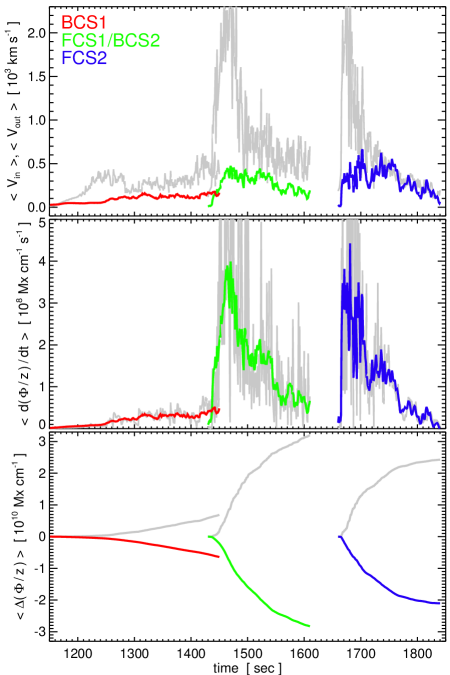
Figure 7: Top panel: Current sheet-averaged inflow velocities $\langle V_{in}\rangle$ (BCS1 red; FCS1/BCS2 green; FCS2 blue) and outflow velocities $\langle V_{out}\rangle$ (gray). Middle panel: Estimate of the CS-averaged reconnection rate magnitude $\langle d(\Phi/z)/dt\rangle$ calculated from the $z$-component of $(\mathbf{V}\times\mathbf{B})$, with the flux into the sheet plotted as the colored lines and flux out of the sheet plotted as gray. Bottom panel: Total change in flux content $\langle\Delta(\Phi/z)\rangle$ due to the signed reconnection rates above.

3.2 Evolution of Current Sheet Reconnection in Physical Units

The top panel of Figure 7 plots CS-averaged $\langle V_{in}\rangle$ (colored lines) and $\langle V_{out}\rangle$ (gray lines) in units of $10^{3}$ km s^-1. The “steady state” inflow speed in BCS1 $\sim$100 km s^-1 while the outflow speeds are $\sim$250 km s^-1 with intermittent periods up to $\sim$400 km s^-1. The FCS1/BCS2 and FCS2 inflow and outflow speeds have a different temporal character than the BCS1 evolution. FCS1/BCS2 and FCS2 inflow speeds are $\sim$300–400 km s^-1 for 80–100 seconds before dropping back down to 100–200 km s^-1. The CS-averaged flare reconnection outflows rapidly reach $\gtrsim$2000 km s^-1 during the period of maximum inflow speed, and drop down to $\sim$600 km s^-1 for FCS1/BCS2 and $\sim$200 km s^-1 for FCS2 as the last of the strong currents dissipate.

The middle panel of Figure 7 plots the time rate of change of the current-sheet averaged flux processed by reconnection, i.e., the $z$-component of the plane-of-the-sky $\mathbf{V}\times\mathbf{B}$ (see Appendix C). The colored lines indicate $\langle d(\Phi/z)/dt\rangle$ calculated with the inflow area averaging procedure and the gray lines correspond to $\langle d(\Phi/z)/dt\rangle$ calculated with the outflow area averaging procedure. The lower panel of Figure 7 plots the time integrated reconnection rates from the above panel, $\langle\Delta(\Phi/z)\rangle=\int dt\langle d(\Phi/z)/dt\rangle$, to show the cumulative flux processed through each of the CS reconnection regions. Again, the total change in flux due to the inflow averaging is shown as the colored lines and the outflow averaging is shown in gray.

L&E13 discussed how, despite the topological similarity between the breakout and flare current sheets, the flare reconnection generates much greater flux transfer rates and inflow/outflow velocity magnitudes because of its fundamentally different roles in the global eruption scenario. The $\langle d(\Phi/z)/dt\rangle$ and $\langle\Delta(\Phi/z)\rangle$ results presented here – calculated directly from the CS regions of the simulation – can be compared to L&E13 Figures 4(c) and 4(b), respectively, where we calculated the same quantities from the evolution of the global flux content in each of the pseudostreamer arcades and newly-formed flare arcades. The peak reconnection rates in FCS1/BCS2 and FCS2 ($\sim$$3\times 10^{8}$ Mx cm^-1 s^-1) are comparable to the L&E13 version, and in both simulations, the maximum flare reconnection rates correspond to approximately 10 times the BCS1 reconnection rate. Likewise, the total flux transfered – measured in L&E13 by following the pseudostreamer arcade separatrices in time and integrating the normal field at the simulation’s lower boundary – agrees reasonably well: $\sim$$6\times 10^{9}$ Mx cm^-1 (BCS1), $\sim$$3\times 10^{10}$ Mx cm^-1 (FCS1/BCS2), and $\sim$$2\times 10^{10}$ Mx cm^-1 (FCS2).

It is worth emphasizing that the method by which the reconnection rate was derived in L&E13 is essentially the procedure used to estimate the reconnection rate from solar observations: one measures the area swept up by the flare ribbons in time and calculates the amount of magnetic flux from the underlying photospheric flux distribution (e.g., Forbes & Lin, 2000; Qiu et al., 2002, 2004; Jing et al., 2005; Kazachenko et al., 2012). The method presented here for deriving the reconnection rate looks exclusively at the field and plasma evolution at the coronal CS regions that are currently extremely difficult to observe. The agreement here with the L&E13 reconnection fluxes is a trivial simulation result (magnetic flux is conserved even when the CS is highly structured, dynamic, and plasmoid unstable) but the implications for the observational flare-ribbon technique as a robust measure of the flux participating in the eruptive flare reconnection is encouraging.

4 Small-Scale Structure in Plasmoid Unstable Current Sheets

4.1 Distributions of Magnetic Island Area, Mass, and Flux Content

To calculate the area of our plasmoid magnetic islands and their mass and flux content, we create a pixel mask associated with each O-type null in every $(x^{\prime},y^{\prime})$ simulation output frame. These masks are constructed by integrating a set of magnetic field lines between the adjacent X-points and only plotting those that belong to the topological domain of the magnetic island, i.e. that do not exceed the spatial position of the bounding X-points. Figure 8 shows a representative pixel mask, one for each CS at the simulation times of Figures 3–5. The island area $A$ is calculated simply by summing the number of non-zero pixels in the mask and multiplying by the pixel area $\delta^{2}=9.54\times 10^{13}$ cm². The island pixel masks multiplied by the mass density and magnetic field components allow us to construct the plasma and flux contents associated with each island (index $o$):

$$A^{o}=\int dA^{o} = \sum_{ij}\delta^{2},$$ (8)

$$(m/z)^{o}=\int\rho\;dA^{o} = \sum_{ij}\delta^{2}\;\rho_{ij},$$ (9)

$$(\psi/z)^{o}=\int\left(\mathbf{B}\cdot\mathbf{\hat{e}_{2}}\right)\;dx^{\prime} \simeq \text@onehalf\sum_{i}\delta\;|\left(\mathbf{B}\cdot\mathbf{\hat{e}_{2}}\right)|_{i,\;j={\rm fixed}}$$ (10)

$$=\int\left(\mathbf{B}\cdot\mathbf{\hat{e}_{1}}\right)\;dy^{\prime} \simeq \text@onehalf\sum_{j}\delta\;|\left(\mathbf{B}\cdot\mathbf{\hat{e}_{1}}\right)|_{i={\rm fixed},\;j}.$$ (11)

Both the plasmoid mass ($m/z$) and plane-of-the-sky flux ($\psi/z$) represent per unit length values, gm cm^-1 and Mx cm^-1, respectively. Here, $i$, $j$, denote the pixel indices in the ($x^{\prime}$, $y^{\prime}$) frame. The island flux content is estimated as the mean of the values obtained from the line integral of the $\mathbf{B}\cdot\mathbf{\hat{e}_{2}}$ magnitude along $dx^{\prime}$ through the island and from the line integral of the $\mathbf{B}\cdot\mathbf{\hat{e}_{1}}$ magnitude along $dy^{\prime}$ through the island. For under-resolved islands ($A\sim$ a few pixels), the planar flux estimates are necessarily approximate. However, for well-resolved islands ($A\gtrsim 10^{2}$ pixels), Equations 10 and 11 yield similar numerical values as expected.

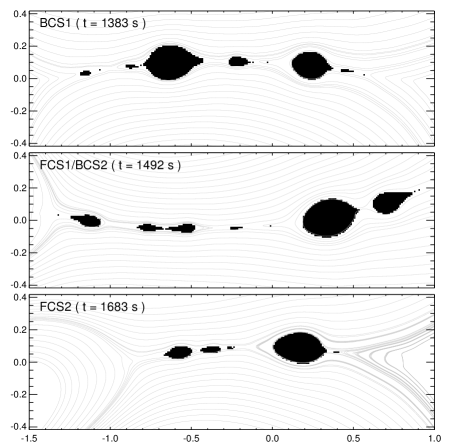
Figure 8: Pixel masks for determining magnetic island area, mass, and flux content for each of the simulation times shown in Figures 3–5.

The probability distributions functions for plasmoid width, flux, and mass content are all derived from their respective cumulative distribution functions (Uzdensky et al., 2010; Shen et al., 2013a). For the magnetic island plasmoid area, the cumulative distribution function $N(A,t)$ measures the number of plasmoids of area $A$ or greater at time $t$. Figure 9 plots the cumulative area distribution as a function of time for each CS where we have used 30 bins spaced uniformly in $\log{A}$ over the range $A\in[1,10^{4}]$ in units of pixel area $\delta^{2}$. The cumulative distribution functions for mass and flux content are likewise calculated and binned over the ranges $m/z\in[10^{-2},10^{6}]$ gm cm^-1 and $\psi/z\in[10^{5},10^{11}]$ Mx cm^-1.

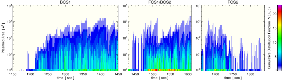
Figure 9: Temporal evolution of the cumulative distribution function of plasmoid area $N(A,t)$ for each of the three current sheets. $N(A,t)$ represents the number of total plasmoids of area $A$ or greater (in units of the pixel area $\delta^{2}=9.54\times 10^{13}$ cm²).

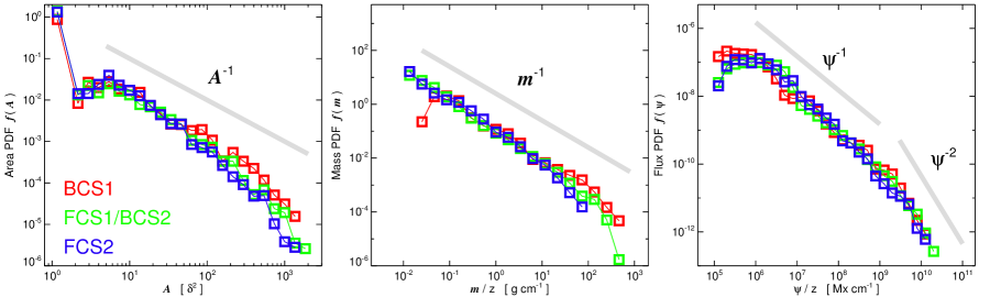
Figure 10: The normalized probability distribution function (PDF) of plasmoid area $f(A)$ (left), mass content $f(m)$ (middle), and average planar flux $f(\psi)$ (right) for each of the three current sheets BCS1 (red), FCS1/BCS2 (green), and FCS2 (blue). Each PDF is constructed from their respective cumulative distribution functions summed over each CS time period. Power law slopes are shown for reference in light gray.

We sum over each of the CS durations ($\tau$) to obtain the cumulative, time-integrated total, $N_{\tau}(A)$. The probability distribution functions are then obtained as $f(A)=-dN_{\tau}(A)/dA$ and correspond to the number of plasmoids per unit area for an area $A$. Here we apply the additional normalization $\Sigma f(A)\Delta A=1$ to ease the comparison between our three cases that generate different numbers of total plasmoids. The left panel of Figure 10 shows the normalized probability density function $f(A)$ calculated for each CS. The middle panel plots the mass density PDF $f(m)=-dN_{\tau}(m/z)/d(m/z)$. The right panel of Figure 10 shows the flux distribution calculated from $f(\psi)=-dN_{\tau}(\psi/z)/d(\psi/z)$. We also plot reference power law slopes for each of the Figure 10 panels as thick light gray lines.

In general, the mass and flux distributions reflect the plasmoid area distribution in each of the three current sheets. This is to be expected if the mass density and upstream field strengths are essentially uniform over the current sheet. For example, if $f(A)\sim A^{-1}$ and the mass content is $m\sim\rho_{0}A$, it follows that $f(m)\sim m^{-1}$. The island area is proportional to an (approximate) island width of $w^{2}$ and therefore our $f(A)\lesssim A^{-1}$ in Figure 10 implies an equivalent $f(w)\lesssim w^{-2}$ scaling. Estimating a planar flux content of $\psi\sim B_{0}w$ yields a flux distribution of $f(\psi)\sim\psi^{-2}$.

Uzdensky et al. (2010) argue that in a stochastic, self-similar plasmoid chain, the fluxes should scale as $f(\psi)\sim\psi^{-2}$ and the island widths, $f(w)\sim w^{-2}$. However, Huang & Bhattacharjee (2012) showed numerical simulations that produce a $\psi^{-1}$ scaling for the flux distribution in magnetic islands, and Fermo et al. (2010) predict an exponential distribution function. Shen et al. (2013a) examined the flux and width distributions of magnetic islands and found qualitatively similar results to Loureiro et al. (2012): the width and flux distributions had slopes between ${-1}$ and ${-2}$ that steepened towards $-2$ for the larger values. Observationally, the distribution of plasmoids in LASCO C2 coronagraph data (density enhancement “upflows” in a post-CME radial plasma sheet) has been investigated by Guo et al. (2013) who found a log-normal shape that was also consistent with an exponential decay for plasmoid widths $\gtrsim 50$ Mm. Lower in the corona, the collimated voids (density depletions) seen by McKenzie & Savage (2011) in flare arcade plasma sheets – called Supra-Arcade Downflows (SADs) – also have an apparent log-normal distribution and recent simulations by Cassak et al. (2013) were used to examine the relationship between SADs and flare reconnection outflows. Likewise, Fermo et al. (2011) showed that Flux Transfer Events observed in the magnetotail by Cluster were also consistent with a log-normal and/or an exponential decay for widths $\gtrsim 4$ Mm.

Our results are consistent with the flatter portion of the Loureiro et al. (2012) and Shen et al. (2013a) distributions and the $\psi^{-1}$ scaling found by Huang & Bhattacharjee (2012). It may be that our choice to dynamically “shorten” the current sheet boundaries over the plasmoids as they approach the end of the sheet means we under-sample the largest plasmoid values and enhance the steepening of the distribution slope at the highest values. Despite this possible selection effect, it is interesting that the largest plasmoids we do count regularly ($A\gtrsim 10^{2}$ pixels) occur in each of the three current sheets. Uzdensky et al. (2010) and Loureiro et al. (2012) have discussed “monster plasmoids” that grow out of the combination of continued reconnected flux accumulation and the coalescence of smaller plasmoids. In our results, the largest plasmoids also reach “macroscopic” sizes, i.e., of order of 10–20% of the total current sheet length ($L\sim 200\delta$), and from Figure 9, are seen to appear, get ejected, and re-appear regularly during a large fraction of both the BCS1 and FCS1/BCS2 time intervals. FCS2 also generates a couple of large plasmoids during the impulsive phase of its eruptive flare before the system relaxation smooths out the reconnection.

4.2 Evolution of the Guide Field Component at the Current Sheets

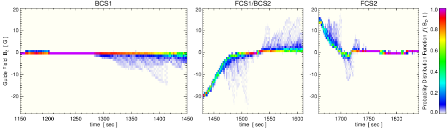
Figure 11: Temporal evolution of the distribution of the guide-field component $B_{z}$ along each current sheet.

Given the differences in the location and the role each current sheet plays in the sympathetic eruption scenario, it is not necessarily obvious that the reconnection and plasmoid properties would agree as much as they do. We calculated the distribution of guide-field flux $(\psi_{z})^{o}=\int B_{z}dA^{o}$ in each island as in $\S$4.1 and found that $f(\psi_{z})\sim\psi_{z}^{-1}$ for exactly the same reasoning ($\psi_{z}\propto A$ for constant $B_{z}$). However, $B_{z}$ does undergo large-scale changes at the CS during reconnection because of the structure and evolution of the sheared fields associated with the eruptions.

Figure 11 plots the distribution of the guide-field $B_{z}$ sampled along each of the CS arcs. Here we have constructed $f(B_{z},t)$ by sampling and binning the $B_{z}(x^{\prime},y^{\prime})$ values along the Appendix B CS arc fits at each output time. The BCS1 $f(B_{z},t)$ distribution is strongly peaked at $B_{z}\sim 0$ but for $t\gtrsim 1300$ s, the reconnecting flux starts to include some of the expanding right-side arcade’s shear component. The process of magnetic island formation also concentrates a relatively weak guide-field component into localized, relatively strong peaks, as seen in the tail of the $f(B_{z},t)$ extending through $-10$ G. FCS1/BCS2 starts deep in the shear channel with $f(B_{z},t)$ highly peaked at $-20$ G and shows a smooth evolution toward zero as the sheared flux reconnects during the eruptive flare and CME formation. Again, once the guide-field magnitude drops below 10 G the plasmoid formation process broadens the tail of the distribution to larger $B_{z}$ values. The FCS1/BCS2 transition between flare reconnection for the first CME and breakout reconnection for the second CME is obvious – the guide field component switches sign from negative to positive $B_{z}$ over $1510\lesssim t\lesssim 1550$ s indicating the sheared flux of the expanding pseudostreamer left-side arcade is now being processed through the CS. After $1550$ s, the FCS1/BCS2 distribution looks similar to BCS1 but with the opposite sign. The FCS2 guide-field distribution starts strongly peaked at the shear channel value of $\sim$15 G and develops the same characteristic distribution broadening as the peak moves towards zero. There is some oscillation in the sign of the weak guide-field values (and thus the extended distribution tails) before FCS2 settles down and the magnetic free energy has been expended.

4.3 Spectral Properties of Current Sheet Magnetic Fluctuations

4.3.1 Wavelet Analysis of Plasmoid Structures

We have performed a wavelet spectral analysis to characterize the spatial scales and power spectra of the magnetic field fluctuations associated with the reconnection-generated magnetic islands in each of our three current sheets. Wavelet analyses have an advantage over traditional spectral methods (Fourier transform) by being able to isolate both large timescale and small timescale periodic behavior that occur over only a subset of the time series (see Edmondson et al., 2013b, and references therein). We sample the simulation data along the CS arc obtained via the method of Appendix B using $x^{\prime}$ as our spatial position parameter to obtain a quantity $Q(x^{\prime})=(B^{2}(x^{\prime})/(8\pi))^{1/2}$. The wavelet transform of $Q$ is defined as

$$W_{Q}(x^{\prime},X)=\int Q(\xi)\Psi^{*}(\xi,x^{\prime},X)d\xi$$ (12)

with the Morlet family waveform given by

$$\Psi^{*}(\xi,x^{\prime},X)=\frac{\pi^{1/4}}{|X|^{1/2}}\exp\left[i\omega_{0}\frac{(\xi-x^{\prime})}{X}\right]\exp\left[-\frac{(\xi-x^{\prime})^{2}}{2X^{2}}\right].$$ (13)

In our application, $\xi$ is the integration variable, $x^{\prime}$ is the position in the CS-centered rectangular frame, and $X$ is the wavelet spatial scale (corresponding to inverse spatial frequency). The non-dimensional frequency parameter $\omega_{0}=6$ corresponds to approximately three oscillations within the Gaussian envelope. The rectified wavelet power spectra is obtained by the square of the wavelet transform amplitude

$$\mathcal{P}_{Q}(x^{\prime},X)=|X|^{-1}|W_{Q}(x^{\prime},X)|^{2}$$ (14)

where we have employed the Liu et al. (2007) frequency scaling to correct for the inherent low-frequency (large spatial scale) bias due to the width of the wavelet filter in frequency space.

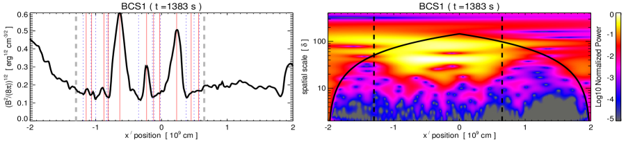
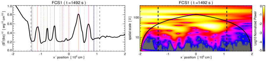
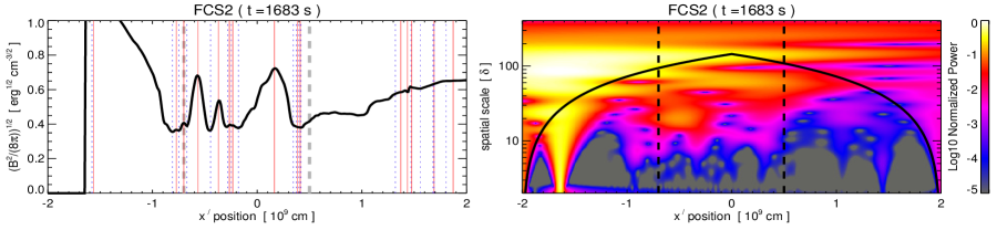
Figure 12: Left column: Sampling of $(B^{2}/(8\pi))^{1/2}$ along the curvilinear arc fits for BCS1 (top row), FCS1/BCS2 (middle row), and FCS2 (bottom row). The CS boundaries are shown as vertical dashed lines and the spatial location of magnetic O-type nulls are shown as vertical red lines, X-type nulls as vertical blue dotted lines. Right column: Wavelet power spectra of each of the corresponding line plot quantities. Animations of this figure are available as electronic supplements to the online version.

The left column of Figure 12 shows the scaled magnetic field magnitude $(B^{2}/(8\pi))^{1/2}$ sampled along the CS arc fits for BCS1, FCS1/BCS2, and FCS2 from top to bottom, respectively. The vertical dashed gray lines indicate the estimates of the CS boundaries $(x^{\prime}_{L},x^{\prime}_{R})$, the location of the O-type nulls are shown as vertical red lines, and the location of X-type nulls are shown as dotted blue lines. The right column of Figure 12 shows the rectified wavelet power distribution at spatial scale size $X$ (in units of grid scale $\delta$) as a function of position $x^{\prime}$ along CS arc for each of the corresponding line plots for each CS.

The largest magnetic islands are clearly visible as enhancements in the magnetic field magnitude line plots and the locations of the O-type nulls (the center of the magnetic islands) occur at the peaks of these enhancements. For the well-resolved large islands, the wavelet transform power shows clear maxima at spatial scales corresponding to the island size, $10\delta\lesssim X\lesssim 40\delta$. The electronic animations of each CS in Figure 12 (FIGURE12_bcs1.mp4, FIGURE12_fcs1.mp4, FIGURE12_fcs2.mp4) show the temporal evolution of the island formation and growth as well as their propagation along the CS arc and ejection in the reconnection exhaust – both in the line plots and in the wavelet power spectra.

4.3.2 Magnetic Energy Density Power Spectra

The global wavelet power spectrum, or the integrated power per scale (IPPS) for the Morlet family of wavelet transforms is roughly equivalent to the global Fourier transform (Le & Wang, 2003; Bolzan et al., 2005). Here we utilize the wavelet transform’s spatial dependence to construct the IPPS spectra of the magnetic energy density along the CS arc in each timeframe only between the boundaries of the CS. While there is still significant structure in the plasmoid quantities just outside of these boundaries, the interaction of the magnetic islands (e.g., reconnection, deformation, etc) with either the line-tied flux system to the left or the CME and/or open flux to the right represent a consequence of the CS evolution rather than an intrinsic part of the reconnection dynamics in the CS itself.

Figure 13 plots the IPPS spectrum for the wavelet power of the magnetic energy density in each CS at the times shown in Figure 12. We define a normalized spatial wavenumber $k_{x^{\prime}}=4L_{0}/X=410\delta/X$ for ease of comparison with the standard Fourier spectral analyses (e.g., Shen et al., 2013a). Recalling $\delta$ is the size of a single computational cell, the maximum wave number of $k_{x^{\prime}}=205$ corresponds to the Nyquist frequency wavelet spatial scale of $X=2\delta$. For the high frequency range of wavenumbers, $15\leq k_{x^{\prime}}\leq 180$, we fit the IPPS spectra with a power law of the form $k_{x^{\prime}}^{-\gamma}$. The power law fit is shown as the thick gray line beneath the IPPS spectra curves for BCS1, FCS1/BCS2, and FCS2 spectra.

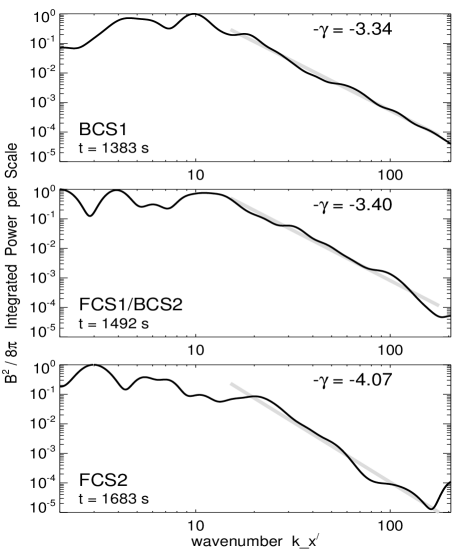
Figure 13: Integrated power per scale (IPPS) spectra of the magnetic energy density wavelet power for BCS1 (top), FCS1/BCS2 (middle), and FCS2 (bottom). The power law fit to the spectra $k_{x^{\prime}}^{-\gamma}$ for wave numbers $15\leq k_{x^{\prime}}\leq 180$ is shown as the thick gray lines.

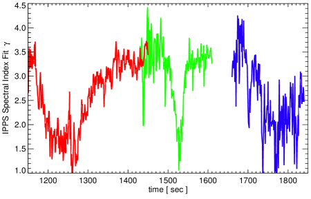
Figure 14: Temporal evolution of the magnetic energy IPPS spectral exponent $\gamma$ for each of our current sheets (BCS1 red; FCS1/BCS2 green; FCS2 blue).

Figure 14 plots the temporal evolution of the spectral index $\gamma$ in the usual color scheme (BCS1 red; FCS1/BCS2 green; FCS2 blue). Overall, our results are in excellent agreement with those presented by Shen et al. (2013a). We see agreement in both the range of the magnetic energy density spectral index $1.5\lesssim\gamma\lesssim 4$ and with their average value of $\gamma\sim 3.5$. The temporal variability of $\gamma$ in our simulation shows moderate fluctuations throughout the evolution of each of our sheets, with periods of the largest variance associated with the rapid reconnection phases in both FCS1/BCS2 and FCS2, but also a slower, more-extended evolution that appears to reflect the global evolution of the CS reconnection dynamics.

The IPPS exponent remains $\sim$2 during the initial development of the X- and O-point chain in BCS1 over the period $1200\lesssim t\lesssim 1300$ s. While this early phase of the current sheet elongation and onset of the plasmoid instability generate an increasing number of islands, the size of these islands remain relatively modest (cf. Figure 9 showing the appearance of only a couple islands with areas exceeding $10^{2}$ pixels through $\sim$1300 s). However, from $t\gtrsim 1300$ s, $\gamma$ increases to the value of $\sim$3.3 There is a noticeable, extended dip in the FCS1/BCS2 $\gamma$ from $\sim$3.5 back to below 2 from about $1510\lesssim t\lesssim 1550$ s even though this period does not have fewer islands (cf. Figure 2) or corresponding changes in macroscopic sheet properties (cf. Figure 6). Inspection of the Figure 4 movie (and also Figure 9) confirms that this period starts with an ejection of a giant island ($A\sim 10^{3}$ pixels) and the remaining islands are relatively small ($A\lesssim 40$ pixels) and do not start to regularly exceed this size again until $t\gtrsim 1550$ s. This period also corresponds to the FCS1/BCS2 transition between the eruptive flare reconnection of the first CME and the overlying breakout reconnection preceding the second CME. The guide-field component ($B_{z}$) is essentially zero here as it switches signs and Figure 11 shows the distribution of $B_{z}$ values in the CS do not have the broadening to larger magnitudes over this interval. Finally, the FCS2 IPPS spectral index also shows the gradual transition from $\gamma\sim 3.5$ down to $\sim$2, but in this case there are corresponding changes in the macroscopic sheet properties, i.e. the dissipation of the strong currents, shrinking of the CS length, and the slowing down of the inflow and outflow speeds. For $t\gtrsim 1740$, the island sizes remain small and the islands themselves are very short-lived. The qualitative behavior and evolution of our IPPS magnetic energy density spectra appears entirely consistent with the physical processes described by Shen et al. (2013a) – the spectra steepens with island growth and merging and becomes shallower with the ejection of the largest islands out of the sheet.

5 Summary and Discussion

We have presented a detailed analysis of the structure and evolution of magnetic islands formed during reconnection in the three large-scale, plasmoid-unstable current sheets associated with the L&E13 sympathetic magnetic breakout eruption scenario. Our current sheets arise naturally and self-consistently from the magnetic topology and evolution of a coronal psuedostreamer as a response to the magnetic free energy introduced by gradual boundary shearing flows and the subsequent rapid re-configuration of the various flux systems during the initiation and eruption of sequential CMEs. The spatial and temporal resolution of the simulation is sufficient to characterize the properties and dynamics of the onset and development of the plasmoid instability in the overlying breakout current sheet and both of the eruptive flare current sheets.

The intermittent, bursty emission that has been observed over a wide range of wavelengths during solar flare events may be related to the structure, dynamics, and evolution of magnetic islands in eruptive flare current sheets (e.g., Kliem et al., 2000; Nakariakov & Melnikov, 2009, and references therein). Pulses of enhanced radiation could originate in discrete acceleration episodes associated with the formation and contraction of magnetic islands during plasmoid-unstable reconnection. In very high-resolution, adaptively-refined simulations of breakout eruptive flare reconnection, Guidoni et al. (2016) have characterized the contraction of different magnetic flux regions inside the MHD simulation islands in order to estimate particle energy gain via the Drake et al. (2006a) mechanism for electron acceleration in plasmoid-unstable current sheets.

It is also important to highlight that in this particular ARMS simulation, our resistivity is entirely numerical. Our results and analysis show that highly structured and detailed reconnection dynamics can be obtained without an explicit, physical resistivity term. The overall qualitative and quantitative properties of the reconnection, i.e. the dimensionless reconnection rate, the magnetic island size, mass, and flux content scaling, the magnetic energy density spectral exponent, are comparable to results obtained via resistive MHD codes, typically run with uniform resistivity.

An important next step in this arena of work will be the forward modeling of synthetic observational signatures of plasmoid formation, structure, and dynamics in the next generation of high-resolution flare current sheet simulations. In particular, numerical MHD simulations with a more realistic treatment of the energy equation using field-aligned thermal conduction, ohmic dissipation, radiative losses, and parameterized coronal heating, would allow for investigation of the detailed thermodynamic evolution within the current sheet, in the magnetic island plasmoids, and the interaction between magnetic islands and flare arcade loops (e.g., Shen et al., 2013b; Downs et al., 2015), and therefore enable a more direct comparison to observations in the low corona.

Appendix A Following the Current Sheets Through the Simulation Domain

Our large scale current sheets are formed in response to the global stresses and evolution of the magnetic field as an integral part of the sympathetic CME eruption scenario from a pseudostreamer topology. As the system evolves, our current sheets move through the simulation domain. For the comparison between the properties of the breakout and eruptive flare current sheets, we have presented each in a similar rectangular $4L_{0}\times 1.333L_{0}$ region centered on the current sheet. The rectangular regions are defined by three time-dependent variables: the spatial coordinates of the rectangular center $x_{c}(t)$, $y_{c}(t)$ and the rotation angle $\alpha(t)$ with respect to the original domain’s $x$-axis. First, we estimate the position of the frame center and its orientation angle by visual inspection of a subset of the images in the Figure 1 movie of $|J|$. We then construct smooth, analytic functions of time based on our initial visual inspection estimates. Thus, the time-evolution of each of our current sheet-centered frames are given by

$${\rm BCS1:}\;\;\;\begin{array}[]{lll}x_{c}(t)&=&-0.0025t+2.8966\\ y_{c}(t)&=&0.00325t+1.7861\\ \alpha(t)&=&6.6\tanh{\left[\frac{t-1335}{50}\right]}+55.4\end{array},$$ (A1)

for $t\in[1150,1450]$ s,

$${\rm FCS1/BCS2:}\;\;\;\begin{array}[]{lll}x_{c}(t)&=&1.15+0.5\left(\frac{t-1430}{180}\right)^{2}\\ &&+0.30\exp{\left[-\left(\frac{t-1560}{30}\right)^{2}\right]}\sin{\left[2\pi\left(\frac{t-1502}{50}\right)\right]}\\ y_{c}(t)&=&4.85-3.5\left(\frac{t-1600}{180}\right)^{2}\\ \alpha(t)&=&105-20\left(\frac{t-1610}{150}\right)^{2}\end{array},$$ (A2)

for $t\in[1430,1610]$ s, and

$${\rm FCS2:}\;\;\;\begin{array}[]{lll}x_{c}(t)&=&0.25-1.2\left(\frac{t-1830}{180}\right)^{2}\\ y_{c}(t)&=&0.875\tanh{\left[\frac{t-1680}{25}\right]}+2.525\\ \alpha(t)&=&27.5\tanh{\left[\frac{1680-t}{50}\right]}+72.5\end{array},$$ (A3)

for $t\in[1661,1841]$ s. Here, $x_{c}$, $y_{c}$ are in units of $L_{0}$ and $\alpha$ is given in degrees.

The transformation from the original simulation coordinates $(x,y)$ to the rectangular current sheet-centered coordinates $(x^{\prime},y^{\prime})$ are given by the standard rotation and translation formula

$$\left[\begin{array}[]{c}x^{\prime}\\ y^{\prime}\end{array}\right]=\left[\begin{array}[]{cc}\cos{\alpha(t)}&\sin{\alpha(t)}\\ \sin{\alpha(t)}&\cos{\alpha(t)}\end{array}\right]\left[\begin{array}[]{c}x-x_{c}(t)\\ y-y_{c}(t)\end{array}\right].$$ (A4)

The left column of Figure 15 plots the rectangular regions centered on the three currents sheets: BCS1 ($t=1383$ s, top row), FCS1/BCS2 ($t=1492$ s, middle row), and FCS2 ($t=1683$ s, bottom row). The right column of Figure 15 plots representative field lines of the current sheet region in the $(x^{\prime},y^{\prime})$ coordinate frames. Figures 3, 4, and 5 show the plasma properties for each of the three current sheets from this perspective at these time periods, respectively.

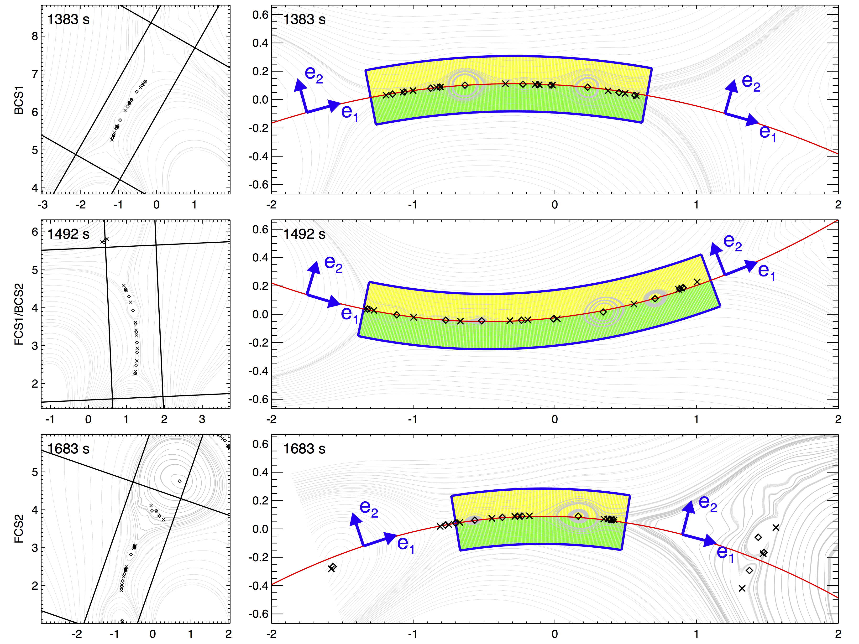
Figure 15: Left column shows the location of the $(x^{\prime},y^{\prime})$ frames centered on the three CS (BCS1 top; FCS1/BCS2 middle; FCS2 bottom) described in Appendix A. The location of X-type nulls (crosses) and O-type nulls (diamonds) are plotted in each panel. Right column plots field lines in the $(x^{\prime},y^{\prime})$ frames along with the curvilinear arc fits $f(x^{\prime}(t_{k}))$ as the thin red lines and the CS region boundaries as thick blue lines (Appendix B). The local current sheet coordinates $(\mathbf{\hat{e}_{1}},\mathbf{\hat{e}_{2}}$) are indicated with unit vectors at representative positions along the curvilinear arc fits in each frame. The upper and lower inflow region areas for calculating CS-averaged quantities are shaded as yellow and green, respectively (Appendix C).

Appendix B Defining a Current Sheet-Centered Curvilinear Coordinate System

While the $(x^{\prime},y^{\prime})$ frames compensate for most of the bulk current sheet motion, Figure 15 also makes clear that the current sheets have large-scale curvature. Thus, we use properties of the current sheet to create a local, spatially-varying curvilinear coordinate system in order to calculate the sheet-averaged quantities, specifically the corrected inflow and outflow velocities. We fit a second-order polynomial to the spatial positions of the null points to obtain the current sheet arc. For the set of X- and O-type null points at location $\{x^{\prime}_{i},y^{\prime}_{i}\}$, we fit a parabola of the form

$$f(x^{\prime})=ax^{\prime 2}+bx^{\prime}+c$$ (B1)

by minimizing the mean square error between the functional fit and the null point locations

$$\chi^{2}=\frac{1}{N}\sum_{i=0}^{N-1}\frac{\left(f(x^{\prime}_{i})-y^{\prime}_{i}\right)^{2}}{\sigma_{i}},$$ (B2)

with weighting factors $\sigma_{i}$ based on spatial position,

$$\sigma_{i}=\left\{\begin{array}[]{ll}0.05&{\rm for}-1\leq x^{\prime}_{i}\leq+1,\\ 0.05+0.15\sin{\left(0.5\pi|x_{i}^{\prime}-1.0|\right)}&{\rm otherwise}.\\ \end{array}\right.$$ (B3)

At times when there are less than 3 null points, we take the CS arc fit to be a horizontal line at the mean $y^{\prime}$ value.

We apply a second, “corrector” step based on the initial $f(x^{\prime})$ fit. At 50 intervals evenly spaced in $x^{\prime}$ we sample $|J|$ in $\pm$10 grid cells in $y^{\prime}$ centered on $f(x^{\prime})$. The spatial locations of $\max{\{|J(x^{\prime},y^{\prime})|\}}$ are then used in the least squared fit of the form of Equations (B1) and (B2) with weightings based on the ratio between the current density magnitude at $x_{i}$ and the maximum $|J|$ over the whole set of $x_{i}$ samples: $\sigma_{i}^{|J|}=0.02\max{\{|J|\}}/|J(x^{\prime}_{i})|$. This allows regions of strong current density in the vicinity of the initial $f(x^{\prime})$ estimate to exert some influence over the arc fit when there are few nearby null points. For example, in the early development of the flare current sheets FCS1/BCS2, FCS2, there is a single X-point but still a well defined current sheet arc.

This procedure works well for the vast majority of the 660 simulation frames analyzed here (300 for BCS1 and 180 each for FCS1/BCS2 and FCS2). However, for some frames, the above fitting procedure clearly misses a portion of the current sheet. In these frames ($t\in\{1465,1471,1478,1678,1748,1749,1760,1761,1775,1786\}$ s) we impose the fit arc parameters by averaging the good fits in the adjacent frames. Occasionally, the $|J|$ corrector step does not improve the arc fit so we keep either the imposed or the original $f(x^{\prime})$ parameters for the following times: $t\in\{1440,1442,1445,1465,1471,1478,1522,1551,1554-1563,1583,1584,1588-1597,1678,1698,1748,1749,1752,1775,1786\}$ s.

As current sheet evolves, the curve defining the CS spatial extent also evolves. Every simulation output time $t_{k}$ has its own parabolic arc $f_{k}=f(x^{\prime}(t_{k}))$ fit to the CS. Each $f_{k}$ defines an instantaneous, local curvilinear coordinate system which can be described by unit vectors $(\mathbf{\hat{e}}_{1},\mathbf{\hat{e}}_{2})$ where $\mathbf{\hat{e}}_{1}(x^{\prime},y^{\prime})$ is tangent to the $f_{k}(x^{\prime})$ curve, $\mathbf{\hat{e}}_{1}\cdot\mathbf{\hat{e}}_{2}=0$, and $\mathbf{\hat{e}}_{1}\times\mathbf{\hat{e}}_{2}=\mathbf{\hat{z}}$:

$$\mathbf{\hat{e}_{1}}(x^{\prime},y^{\prime}) = \frac{1}{\sqrt{1+\left(\frac{df_{k}}{dx^{\prime}}\right)^{2}}}\left(\mathbf{\hat{x}^{\prime}}+\frac{df_{k}}{dx^{\prime}}\mathbf{\hat{y}^{\prime}}\right),$$ (B4)

$$\mathbf{\hat{e}_{2}}(x^{\prime},y^{\prime}) = \frac{1}{\sqrt{1+\left(\frac{df_{k}}{dx^{\prime}}\right)^{2}}}\left(-\frac{df_{k}}{dx^{\prime}}\mathbf{\hat{x}^{\prime}}+\mathbf{\hat{y}^{\prime}}\right).$$ (B5)

The right column of Figure 15 plots the location of the X-type and O-type nulls (as crosses and diamonds), the $f_{k}(x^{\prime})$ arc fit as the red line, and $(\mathbf{\hat{e}}_{1},\mathbf{\hat{e}}_{2})$ unit vectors at two representative positions along $f_{k}(x^{\prime})$ to illustrate their spatial dependence. The boundary of the CS region is highlighted as thick blue lines, and each of the inflow regions shaded as yellow and green.

The total current sheet length $2L(t)$ is obtained via standard arc length integration between our estimates of the CS boundaries, $x^{\prime}_{L}$ to $x^{\prime}_{R}$, at each simulation output frame $t_{k}$,

$$2L(t_{k})=\int_{x^{\prime}_{L}(t_{k})}^{x^{\prime}_{R}(t_{k})}dx^{\prime}\sqrt{1+\left(\frac{df_{k}}{dx^{\prime}}\right)^{2}}.$$ (B6)

The half-length $L(t_{k})$ is used in the calculation of the CS aspect ratio $L(t)/\delta$ shown the top panel of Figure 6. The ($x^{\prime}_{L}$, $x^{\prime}_{R}$) current sheet boundaries were obtained via visual inspection of every other simulation time output frame ($t_{k}$ even) and the positions during $t_{k}$ odd simulation times were linearly interpolated between the positions of the adjacent even times. The estimate of the CS boundaries were guided by the opening angle of the field lines made with respect to the parabolic arc fit.

Appendix C Constructing Current Sheet-Averaged Quantities

The local, spatially-varying CS curvilinear coordinates defined by Equations B4, B5 are used to decompose the velocity and magnetic field vectors into components tangent to ($\mathbf{\hat{e}}_{1}$) and perpendicular to ($\mathbf{\hat{e}}_{2}$) the current sheet. The precise inflow and outflow velocities are given by $V_{in}^{\pm}=\pm(\mathbf{V}\cdot\mathbf{\hat{e}}_{2})$ and $V_{out}^{\pm}=\pm(\mathbf{V}\cdot\mathbf{\hat{e}}_{1})$, where the $\pm$ notation indicates the positive, negative $\mathbf{\hat{e}}_{1}$, $\mathbf{\hat{e}}_{2}$ directions respectively: i.e., inflow into the sheet from ‘above’ $(-)$ and ‘below’ $(+)$, and outflow from the sheet to the ‘left’ $(-)$ and ‘right’ $(+)$.

To obtain the sheet-averaged quantities, we construct the mean ‘above’ and ‘below’ inflow components $\langle V_{in}^{-}\rangle$, $\langle V_{in}^{+}\rangle$ by averaging the $\mathbf{V}\cdot\mathbf{\hat{e}}_{2}$ values in the yellow and green regions shown in Figure 15. The inflow regions are defined by a distance of 20 grid points in the direction of $\pm\mathbf{\hat{e}}_{2}$ starting from $(x^{\prime},f(x^{\prime}))$ over the range of the CS boundaries $x^{\prime}\in[x^{\prime}_{L},x^{\prime}_{R}]$. We also construct the mean ‘left’ and ‘right’ outflow velocities, $\langle V_{out}^{-}\rangle$ and $\langle V_{out}^{+}\rangle$ in an analogous fashion from the $\mathbf{V}\cdot\mathbf{\hat{e}}_{1}$ values. Here we take a single line of $\pm$5 grid points in the $\mathbf{\hat{e}}_{2}$ direction centered on $(x^{\prime}_{L},f(x^{\prime}_{L}))$ for the ‘left’ boundary and $(x^{\prime}_{R},f(x^{\prime}_{R}))$ for the ‘right’ boundary. In both the inflow and outflow cases, the $(+)$ and $(-)$ values have the opposite sign, so we average the two sets of magnitudes to get the CS-averaged quantities:

$$\langle V_{in}\rangle = \text@onehalf\left(\langle V_{in}^{+}\rangle+\langle V_{in}^{-}\rangle\right),$$ (C1)

$$\langle V_{out}\rangle = \text@onehalf\left(\langle V_{out}^{+}\rangle+\langle V_{out}^{-}\rangle\right).$$ (C2)

These quantities are plotted for each of the current sheets in the top panel of Figure 7 and their ratio $\langle V_{in}\rangle/\langle V_{out}\rangle$ is shown in the bottom panel of Figure 6.

The magnetic field can also be decomposed into components parallel ($\mathbf{B}\cdot\mathbf{\hat{e}}_{1}$) and perpendicular ($\mathbf{B}\cdot\mathbf{\hat{e}}_{2}$) to the current sheet. We can estimate the current sheet-averaged time rate of change in flux associated with the inflow region by starting with the induction equation (4), taking an area integral ($d\mathbf{A}=de_{2}dz\mathbf{\hat{e}}_{1}$), and applying Stokes’ theorem:

$$\int d\mathbf{A}\cdot\frac{\partial\mathbf{B}}{\partial t} = \int d\mathbf{A}\cdot\nabla\times\left(\mathbf{V}\times\mathbf{B}\right)$$

$$\frac{\partial}{\partial t}\int dA\left(\mathbf{B}\cdot\mathbf{\hat{e}}_{1}\right) = \oint d\boldsymbol{\ell}\cdot\left(\mathbf{V}\times\mathbf{B}\right).$$ (C3)

Utilizing a convenient choice of area, the line integral can be constructed to give the familiar result in terms of the $z$-component of ($\mathbf{V}\times\mathbf{B}$):

$$\frac{d(\Phi_{in}/z)}{dt}=\left(\mathbf{V}\cdot\mathbf{\hat{e}}_{1}\right)\left(\mathbf{B}\cdot\mathbf{\hat{e}}_{2}\right)-\left(\mathbf{V}\cdot\mathbf{\hat{e}}_{2}\right)\left(\mathbf{B}\cdot\mathbf{\hat{e}}_{1}\right).$$ (C4)

Likewise, the change in flux from the outflow is calculated with the area ($d\mathbf{A}=de_{1}dz\mathbf{\hat{e}}_{2}$) and its corresponding line integral to obtain

$$\frac{d(\Phi_{out}/z)}{dt}=-\left(\mathbf{V}\cdot\mathbf{\hat{e}}_{1}\right)\left(\mathbf{B}\cdot\mathbf{\hat{e}}_{2}\right)+\left(\mathbf{V}\cdot\mathbf{\hat{e}}_{2}\right)\left(\mathbf{B}\cdot\mathbf{\hat{e}}_{1}\right).$$ (C5)

We then apply the spatial averaging procedure described above for the upper and lower portions of the inflow region to obtain $\langle d(\Phi_{in}/z)/dt\rangle$ and along the left and right arc boundaries to obtain $\langle d(\Phi_{out}/z)/dt\rangle$ (see middle panel of Figure 7). The total fluxes transferred through the sheet via inflow and outflow are simply calculated as $\langle\Delta(\Phi/z)\rangle=\int dt\;\langle d(\Phi/z)/dt\rangle$, shown in the bottom panel of Figure 7.

References

- Antiochos et al. (1999) Antiochos, S. K., DeVore, C. R., & Klimchuk, J. A. 1999, ApJ, 510, 485
- Antiochos et al. (2002) Antiochos, S. K., Karpen, J. T., & DeVore, C. R. 2002, ApJ, 575, 578
- Aulanier et al. (2002) Aulanier, G., DeVore, C. R., & Antiochos, S. K. 2002, ApJ, 567, L97
- Aulanier et al. (2006) Aulanier, G., DeVore, C. R., & Antiochos, S. K. 2006, ApJ, 646, 1349
- Bhattacharjee et al. (2009) Bhattacharjee, A., Huang, Y.-M., Yang, H., & Rogers, B. 2009, Phys. Plasmas, 16, 112102
- Birn et al. (2001) Birn, J., Drake, J. F., Shay, M. A., Rogers, B. N., Denton, R. E., Hesse, M., Kuznetsova, M., Ma, Z. W., Bhattacharjee, A., Otto, A., & Pritchett, P. L. 2001, J. Geophys. Res., 106, A3, 3715
- Birn & Hesse (2001) Birn, J., & Hesse, M. 2001, J. Geophys. Res., 106, A3, 3737
- Biskamp (1986) Biskamp, D. 1986, Phys. Fluids, 29, 1520
- Biskamp (1996) Biskamp, D. 1996, Ap&SS, 242, 165
- Bolzan et al. (2005) Bolzan, M., Rosa, R. R., Ramos, F. M., Fagundes, P.R., & Sahai,Y. 2005, JASTP, 67, 1843
- Canfield et al. (2007) Canfield, R. C., Kazachenko, M. D., Acton, L. W., et al. 2007, ApJ, 671, L81
- Carmichael (1964) Carmichael, H. 1964, in The Physics of Solar Flares, NASA SP-50, ed. W. N. Hess (Washington DC: NASA), 451
- Cassak et al. (2013) Cassak, P., Drake, J. F., Gosling, J. T., Phan, T.-D., Shay, M. A., & Shepherd, L. S. 2013, ApJ, 775, L14
- Cassak & Drake (2013) Cassak, P., & Drake, J. F. 2013, Phys. Plasmas, 20, 061207
- Cassak et al. (2009b) Cassak, P., Shay, M. A., & Drake, J. F. 2009, Phys. Plasmas, 16, 120702
- DeVore (1991) DeVore, C. R. 1991, J. Comput. Phys., 92, 142
- DeVore & Antiochos (2008) DeVore, C. R., & Antiochos, S. K. 2008, ApJ, 680, 740
- Daughton et al. (2006) Daughton, W., Scudder, J., & Karimabadi, H. 2006, Phys. Plasmas, 13, 072101
- Daughton et al. (2009) Daughton, W., Roytershteyn, V., Albright, B. J., Karimabadi, H., Yin, L., & Bowers, K. J. 2009, Phys. Rev. Lett., 103, 065004
- Downs et al. (2015) Downs, C., Török, T., Titov, V., Liu, W., Linker, J., & Mikić, Z. 2015, AAS/AGU Triennial Earth-Sun Summit, 1, #304.01
- Drake et al. (2006a) Drake, J. F., Swisdak, M., Che, H., & Shay, M. A. 2006a, Nature, 443, 553
- Drake et al. (2006b) Drake, J. F., Swisdak, M., Schoeffler, K. M., Rogers, B. N., & Kobayashi, S. 2006b, Geophys. Res. Lett., 33, L13105
- Edmondson et al. (2010) Edmondson, J. K., Antiochos, S. K., DeVore, C. R., & Zurbuchen, T. H. 2010, ApJ, 718, 72
- Edmondson et al. (2009) Edmondson, J. K., Lynch, B. J., Antiochos, S. K., De Vore, C. R., & Zurbuchen, T. H. 2009, ApJ, 707, 1427
- Edmondson et al. (2013b) Edmondson, J. K., Lynch, B. J., Lepri, S. T., & Zurbuchen, T. H. 2013b, ApJS, 209, 35
- Fermo et al. (2010) Fermo, R. L., Drake, J. F., & Swisdak, M., Phys. Plasmas, 17, 010702
- Fermo et al. (2011) Fermo, R. L., Drake, J. F., Swisdak, M., & Hwang, K.-J. 2011, J. Geophys. Res., 116, A09225
- Forbes & Isenberg (1991) Forbes, T. G., & Isenberg, P. A. 1991, ApJ, 373, 294
- Forbes & Lin (2000) Forbes, T. G., & Lin, J. 2000, J. Atm. Sol.-Terr. Phys., 62, 1499
- Forbes & Malherbe (1991) Forbes, T. G., & Malherbe, J. M. 1991, Sol. Phys., 135, 361
- Forbes & Priest (1983) Forbes, T. G., & Priest, E. R. 1983, Sol. Phys., 84, 169
- Furth et al. (1963) Furth, H. P., Killeen, J., & Rosenbluth, M. N. 1963, Phys. Fluids, 6, 459
- Gibson & Fan (2006) Gibson, S. E., & Fan, Y. 2006, J. Geophys. Res., 111, A12103
- Green & Kliem (2009) Green, L. M., & Kliem, B. 2009, ApJ, 700, L83
- Guidoni et al. (2016) Guidoni, S. E., DeVore, C. R., Karpen, J. T., & Lynch, B. J. 2016, ApJ, 820, 60
- Guo et al. (2013) Guo, L.-J., Bhattacharjee, A., & Huang, Y.-M. 2013, ApJ, 771, L14
- Hesse et al. (2001) Hesse, M., Birn, J., & Kuznetsova, M. 2001, J. Geophys. Res., 106, A3, 3721
- Hirayama (1974) Hirayama, T. 1974, Sol. Phys. 34, 323
- Huang & Bhattacharjee (2010) Huang, Y.-M., & Bhattacharjee, A. 2010, Phys. Plasmas, 17, 062104
- Huang & Bhattacharjee (2012) Huang, Y.-M., & Bhattacharjee, A. 2012, Phys. Rev. Lett., 109, 265002
- Isenberg & Forbes (2007) Isenberg, P. A., & Forbes, T. G. 2007, ApJ, 670, 1453
- Jing et al. (2005) Jing, J., Qiu, J., Lin, J., Qu, M., Xu, Y., & Wang, H., ApJ, 620, 1085
- Karpen et al. (1995) Karpen, J. T., Antiochos, S. K., & DeVore, C. R. 1995, ApJ, 450, 422
- Karpen et al. (2012) Karpen, J. T., Antiochos, S. K., & DeVore, C. R. 2012, ApJ, 760, 81
- Karpen et al. (1998) Karpen, J. T., Antiochos, S. K., DeVore, C. R., & Golub, L. 1998, ApJ, 495, 491
- Kazachenko et al. (2012) Kazachenko, M. D., Canfield, R. C., Longcope, D. W., & Qiu, J. 2012, Sol. Phys., 277, 165
- Kliem et al. (2000) Kliem, B., Karlický, M., & Benz, A. O. 2000, A&A, 360, 715
- Kopp & Pneuman (1976) Kopp, R. A., & Pneuman, G. W. 1976, Sol. Phys., 50, 85
- Kuznetsova et al. (2001) Kuznetsova, M., Hesse, M., & Winske, D. 2001, J. Geophys. Res., 106, A3, 3799
- Le & Wang (2003) Le, G.-M., & Wang, J.-L. 2003, ChJAA, 3, 391
- Lin et al. (2009) Lin, J., Li, J., Ko, Y.-K., & Raymond, J. C. 2009, ApJ, 693, 1666
- Liu et al. (2007) Liu, Y., San Liang, X., & Weisberg, R. H. 2007, JAtOT, 24, 2093
- Loureiro et al. (2012) Loureiro, N. F., Samtaney, R., Schekochikin, A. A., & Uzdensky, D. A. 2012, Phys. Plasmas, 19, 042303
- Loureiro et al. (2007) Loureiro, N. F., Schekochihin, A. A., & Cowley, S. C. 2007, Phys. Plasmas, 14, 100704
- Lynch et al. (2008) Lynch, B. J., Antiochos, S. K., DeVore, C. R., Luhmann, J. G., & Zurbuchen, T. H. 2008, ApJ, 683, 1192
- Lynch & Edmondson (2013) Lynch, B. J., & Edmondson, J. K. 2013, ApJ, 764, 87
- Ma & Bhattacharjee (2001) Ma, Z. W., & Bhattacharjee, A. 2001, J. Geophys. Res., 106, A3, 3773
- MacNeice et al. (2004) MacNeice, P., J., Antiochos, S. K., Phillips, A., Spicer, D. S., DeVore, C. R., & Olson, K. 2004, ApJ, 614, 1028
- MacNeice et al. (2000) MacNeice, P. J., Olson, K. M., Mobarry, C., de Fainchtein, R., & Packer, C. 2000, Comput. Phys. Commun., 126, 330
- Manchester et al. (2004) Manchester, W. B., IV, Gombosi, T. DeZeeuw, D., & Fan, Y. 2004, ApJ, 610, 588
- Manchester (2008) Manchester, W. B., IV, in ASP Conf. Ser. 383, Subsurface and Atmospheric Influences on Solar Activity, ed. R. Howe, R. W. Komm, K. S. Balasubramaniam & G. J. D. Petrie. (San Francisco, CA: ASP), 91
- Masson et al. (2013) Masson, S., Antiochos, S. K., & DeVore, C. R. 2013, ApJ, 771, 82
- McKenzie & Savage (2011) McKenzie, D. E., & Savage, S. L. 2011, ApJ, 735, L6
- Murphy et al. (2010) Murphy, N. A. 2010, Phys. Plasmas, 17, 112310
- Murphy et al. (2013) Murphy, N. A., Young, A. K., Shen, C., Lin, J., & Ni, L. 2013, Phys. Plasmas, 20, 061211
- Nakariakov & Melnikov (2009) Nakariakov, V. M., & Melnikov, V. F. 2009, Space Sci. Rev., 149, 119
- Ni et al. (2010) Ni, L, Germaschewski, K., Huang, Y.-M., Sullivan, B. P., Yang, H., & Bhattacharjee, A. 2010, Phys. Plasmas, 17, 052109
- Otto (2001) Otto, A. 2001, J. Geophys. Res., 106, A3, 3751
- Parker (1963) Parker, E. N. 1963, ApJS, 8, 177
- Pariat et al. (2009) Pariat, E., Antiochos, S. K., & DeVore, C. R., 2009, ApJ, 691, 61
- Pariat et al. (2010) Pariat, E., Antiochos, S. K., & DeVore, C. R. 2010, ApJ, 714, 1762
- Petschek (1964) Petschek, H. E. 1964, in The Physics of Solar Flares, NASA SP-50, ed. W. N. Hess (Washington DC: NASA), 425
- Pritchett (2001) Pritchett, P. L. 2001, J. Geophys. Res., 106, A3, 3783
- Qiu et al. (2002) Qiu, J., Lee, J., Gary, D. E., & Wang, H. 2002, ApJ, 565, 1335
- Qiu et al. (2004) Qiu, J., Wang, H., Cheng, C. Z., & Gary, D. E. 2004, ApJ, 604, 900
- Savcheva et al. (2012a) Savcheva, A. S., Green, L. M., van Ballegooijen, A. A., & DeLuca, E. E. 2012a, ApJ, 759, 105
- Savcheva et al. (2012b) Savcheva, A. S., Pariat, E., van Ballegooijen, A. A., Aulanier, G., & DeLuca, E. E. 2012b, ApJ, 750, 15
- Samtaney et al. (2009) Samtaney, R., Loureiro, N. F., Uzdensky, D. A., Schekochihin, A. A., & Cowley, S. C. 2009, Phys. Rev. Lett. 103, 105004
- Shay et al. (2001) Shay, M. A., Drake, J. F., Rogers, B. N., & Denton, R. E. 2001, J. Geophys. Res., 106, A3, 3759
- Shen et al. (2011) Shen, C., Lin, J., & Murphy, N. A. 2011, ApJ, 737, 14
- Shen et al. (2013a) Shen, C., Lin, J., Murphy, N. A., & Raymond, J. C. 2013a, Phys. Plasmas, 20, 072114
- Shen et al. (2013b) Shen, C., Reeves, K. K., Raymond, J. C., Murphy, N. A., Ko, Y.-K., Lin, J., Mikić, Z., & Linker, J. A. 2013b, ApJ, 773, 110
- Sterling (2001) Sterling, A. C., Hudson, H. S., Thompson, B. J., & Zarro, D. M. 2001, ApJ, 532, 628
- Sturrock (1966) Sturrock, P. A. 1966, Nature, 211, 695 697
- Sweet (1958) Sweet, P. A. 1958, in Electromagnetic Phenomena in Cosmic Physics, ed. B. Lehnert (New York: Cambridge University Press), 123
- Syrovatskii (1971) Syrovatskii, S. I. 1971, Sov. J. Exp. Theor. Phys., 33, 933
- Syrovatskii (1978a) Syrovatskii, S. I. 1978a, Astrophys. Space Sci., 56, 3
- Syrovatskii (1978b) Syrovatskii, S. I. 1978b, Sol. Phys., 58, 89
- Syrovatskii (1981) Syrovatskii, S. I. 1981, ARA&A, 19, 163
- Titov & Démoulin (1999) Titov, V. S., & Démoulin, P. 1999, A&A, 351, 707
- Török et al. (2011) Török, T., Panasenco, O., Titov, V. S., Mikić, Z., Reeves, K. K., Velli, M., Linker, J. A., & De Toma, G. 2011, ApJ, 739, L63
- Uzdensky et al. (2010) Uzdensky, D. A., Loureiro, N. F., & Schekochihin, A. A. 2010, Phys. Rev. Lett. 105, 235002
- Welsch et al. (2005) Welsch, B. T., DeVore, C. R., & Antiochos, S. K. 2005, ApJ, 634, 1395