Into the third dimension: stochastic measurements of Stokes parameters within the Poincaré sphere

Inspired by recent use of polarimetry to study the Cosmic Microwave Background and extragalatic supernovae, a foray into the statistical properties of Stokes parameters expressed in spherical coordinates is began, allowing circular polarization and linear polarization to be treated in a unified manner. The use of spherical coordinates is quite necessary as it permits a Stokes polarization state to be expressed in terms of the customary polarization angles and degree of polarization usually needed for human interpretation. As shall be demonstrated, circular and linear polarization are not statistically independent quantities but intertwined in a way that is especially important, for instance, at low signal-to-noise. New distributions, classical estimators, and marginalizations are presented for this “three-dimensional” polarization problem including a generalization of the Rice distribution. The paper concludes with discussion regarding the potential pitfalls of a lower dimensional analysis.

1 Introduction

Astronomical polarimetry and spectropolarimetry, which have historically been under-utilized, are now routinely being used in many experiments to search for and test new physics. Besides the diverse application of polarimetric techniques in solar and stellar astronomy, two areas of particular note are polarimetric observations of the Cosmic Microwave Background (CMB) and spectropolarimetric observations of supernovae (SNe).

Detection of inflation signatures on the CMB using polarimetric imaging were recently announced by the BICEP2 team (Ade et al., 2014b, a). This result would confirm one of astrophysics most cherished but experimentally elusive theories. After a review of the public BICEP2 data, some have questioned the interpretation of the BICEP2 data and suggested that the foreground dust contamination had been underestimated or that the signal could have been produced by other mechanisms such as “radio loops” (Liu et al., 2014). The BICEP2 team have stood by their results although they have moderated their language in the peer-reviewed version of their paper (Ade et al., 2014b). If valid, the BICEP2 discovery continues the trend set by all-sky mapping satellites like COBE, WMAP, and Planck and various ground and balloon surveys of the CMB being perhaps the single most fruitful source to test cosmological theory and sometimes even fundamental physics. Further results related to CMB polarization are expected in the near future from BICEP3 (Kuo & BICEP3 and POLAR1 Collaborations, 2013), the Keck Array (Staniszewski et al., 2012), POLARBEAR (The POLARBEAR Collaboration, 2014), and the Planck team (Planck Collaboration, 2014). It is clear that the CMB will continue to be a vital source of cutting edge science; but, as the controversy around the BICEP2 announcement indicates, polarization work is tricky and extreme care must be made to handle properly statistical and systematic error in the data.

Other research groups have been using spectropolarimetric observations to investigate the systematic behavior and statistical variation of thermonuclear (Type Ia) and core-collapse SNe (all other types) arising from asymmetries. (The Wang & Wheeler (2008) Annual Review is a good introduction.) Spectropolarimetry is the only known way to probe asymmetries of unresolved sources such as extra-galactic supernovae so it will continue to be an effective research tool. The detection of asymmetries has helped place much needed constraints on SNe explosion physics/progenitor scenarios (recent examples include Maund et al. (2010b); Tanaka et al. (2012); Patat et al. (2012); Zelaya et al. (2013); Maund et al. (2013)) and environments (Mauerhan et al., 2014). Asymmetries of Type Ia SNe are of particular interest as high-redshift events were famously used to discover cosmic acceleration (Riess et al., 1998; Perlmutter et al., 1999), a result for which leads of two large teams shared the 2011 Nobel Prize. This acceleration implies the existence of so-called “dark energy”, whose physical nature is completely puzzling and is perhaps the biggest unsolved problem in astrophysics. As such, any possible correlations between metrics of asymmetry in Type Ia SNe and other observables (Leonard et al., 2005; Wang et al., 2007; Maund et al., 2010a) are of high importance because correlations may be used to identify contaminating Type Ia sub-classes (Wang et al., 2013) or apply statistical corrections to the maximum brightness, both of which could help refine the measurement of the cosmological constant (Maeda et al., 2011). Spectropolarimetry of SNe is a blooming field but, just as with the CMB, handling the statistical and systematic error of polarimetric data for SNe is challenging.

As both polarimetric imaging and spectropolarimetry require dividing incoming light into bins, researchers in these fields often find themselves in photon-starved situations. Indeed, in both subjects discussed above, photon-limited data at low signal-to-noise must be confronted. (Low signal-to-noise is often the hallmark of forefront science by its very nature.) This problem is compounded in polarimetric imaging when a narrow-band filter is needed. Working at low signal-to-noise will continue to be an issue for polarimetrists.

Polarization data is often measured in Stokes parameters but expressed in human-digestible quantities like degrees of polarization and angles of polarization. Despite this, there has been relatively little attention given to the surprisingly complicated statistics involved when making transformations to these quantities at low signal-to-noise. Most of the published literature of this fundamental, practical topic has focused on the analysis of linear polarization alone that involves marginalizations over a two-dimensional gaussian distribution over the $Q$-$U$ plane cross section of the Poincaré sphere (the “Poincaré disk” is a useful expression although it is already in use in other mathematical contexts). Marginalization over linear degree of polarization results in the Rice distribution (Rice, 1945) while marginalization over the linear polarization angle results in another distribution given by Vinokur (1965). The authors refer to this marginalized approach as the “one-dimensional problem”. A small number of papers such as Wang et al. (1997), Vaillancourt (2006), and Quinn (2012) have used a non-marginalized distribution over the Poincaré disk (the “two-dimensional problem”), with the latter being the first to put the subject on a rigorous mathematical footing. To date, there has been little to no attention paid to the three-dimensional problem defined by a three-dimensional distribution over the Poincaré sphere. Progress on higher dimensional generalizations of the two-dimensional problem have been made, for instance, by members of the Planck Collaboration (Planck Collaboration (2014); Montier et al. (2014a, b)) by including intensity in the analysis but researchers have thus far generally ignored circular polarization when measuring linear polarization in astronomical sources (and vice versa); however, the measurement of one is not actually independent of the other. This effect is generally negligible except when one is working at very small signal-to-noise ratios or with objects with polarization near 100% (see Quinn (2012) for details on how large polarization introduces complication). The aim of this paper is to elucidate some of this interdependence and to see how it relates to the more common ways of treating linear polarization measurements at low signal-to-noise via the Rice distribution or through Bayesian techniques as outlined in Vaillancourt (2006) and Quinn (2012). The results should be of interest to all polarimetrists and those those studying the CMB or SNe in particular.

2 The sampling distribution

A very practical way of encoding the polarization state of electromagnetic radiation is the Stokes parameter formalism invented by George Stokes in 1852. Stokes parameters consist of four quantities: $I$ (intensity), $Q$ and $U$ (related to linear polarization), and $V$ (related to circular polarization). They are convenient quantities to measure but it is easier for people to think about polarization in terms of percentages and angles. This may be done by introducing a spherical coordinate system $(p,\theta,\phi)$ on points of the Poincaré sphere (a unit ball in Cartesian coordinates centered on the origin of $\frac{Q}{I_{0}}$, $\frac{U}{I_{0}}$, and $\frac{V}{I_{0}}$ axes), which represents all possible polarization states. Accessible modern introductions to Stokes parameters and their theory are given in del Toro Iniesta (2003) and Landi Degl’Innocenti (2002).

If an astronomical source’s polarization state is measured with gaussian error $(\Sigma_{I},\Sigma_{Q},\Sigma_{U},\Sigma_{V})$ on each Stokes parameter $(I,Q,U,V)$, how do the corresponding spherical coordinates $(p,\theta,\phi)$ relate to the “true” polarization state $(p_{0},\theta_{0},\phi_{0})$ determined uniquely from $(I_{0},Q_{0},U_{0},V_{0})$? (Unsubscripted variables will usually refer to measured values while “0”-subscripted values will refer to “true” values. Later, an overbar on some variables and distributions will indicate signal-to-noise related quantities.) As it turns out, a spherical coordinate system introduces non-trivial biases into the measured quantities and the measurement itself must be “corrected” to remove them. This paper extends Quinn (2012), which studied these effects in polar coordinates before discussing the Bayesian approach, to spherical coordinates. The reader is referred to that paper for a more extensive introduction on Stokes parameters.

Under the assumptions that the source intensity is large compared to the measurement error, i.e., $I_{0}\gg\Sigma_{I}$ which implies $I\approx I_{0}$ (Quinn, 2012), and the error on a Stokes measurement is described by a three-dimensional uncorrelated ellipsoidal Gaussian distribution (with semi-major axes $\Sigma_{Q}$, $\Sigma_{U}$, $\Sigma_{V}$), the normalized distribution, $F_{C}$, of the measured Stokes parameters ($Q$, $U$, $V$) given the “true” Stokes parameters ($Q_{0}$, $U_{0}$, $V_{0}$) is

$$\begin{split}F_{C}(Q,U,V|Q_{0},U_{0},{}&V_{0},\Sigma_{Q},\Sigma_{U},\Sigma_{V})=\\ &\frac{1}{(2\pi)^{3/2}\Sigma_{Q}\Sigma_{U}\Sigma_{V}}e^{-\left(\frac{(Q-Q_{0})^{2}}{2\Sigma_{Q}^{2}}+\frac{(U-U_{0})^{2}}{2\Sigma_{U}^{2}}+\frac{(V-V_{0})^{2}}{2\Sigma_{V}^{2}}\right)}.\end{split}$$ (1)

These parameters are not usually worked with directly. Instead “normalized Stokes parameters” are defined as $q\equiv Q/I_{0}$, $u\equiv U/I_{0}$, $v\equiv V/I_{0}$ (with also $q_{0}\equiv Q_{0}/I_{0}$, $u_{0}\equiv U_{0}/I_{0}$, and $v_{0}\equiv V_{0}/I_{0}$), and $\sigma_{q}\equiv\Sigma_{Q}/I_{0}$, $\sigma_{u}\equiv\Sigma_{U}/I_{0}$, and $\sigma_{v}\equiv\Sigma_{V}/I_{0}$, yielding a new normalized distribution

$$\begin{split}f_{C}(q,u,v|q_{0},u_{0},v_{0},\sigma_{q},{}&\sigma_{u},\sigma_{v})=\\ &\frac{1}{(2\pi)^{3/2}\sigma_{q}\sigma_{u}\sigma_{v}}e^{-\left(\frac{(q-q_{0})^{2}}{2\sigma_{q}^{2}}+\frac{(u-u_{0})^{2}}{2\sigma_{u}^{2}}+\frac{(v-v_{0})^{2}}{2\sigma_{v}^{2}}\right)}.\end{split}$$ (2)

Lastly, one most often works with “signal-to-noise” versions of the Stokes parameters defined as $\overline{q}\equiv Q/\Sigma_{Q}=q/\sigma_{q}$, $\overline{u}\equiv U/\Sigma_{U}=u/\sigma_{u}$, and $\overline{v}\equiv V/\Sigma_{V}=v/\sigma_{v}$ which gives another distribution

$$\begin{split}\overline{f}_{C}(\overline{q},\overline{u},\overline{v}|\overline{q}_{0},\overline{u}_{0},\overline{v}_{0},\sigma_{q},\sigma_{u},{}&\sigma_{v})=\\ &\frac{1}{(2\pi)^{3/2}}e^{-\frac{(\overline{q}-\overline{q}_{0})^{2}+(\overline{u}-\overline{u}_{0})^{2}+(\overline{v}-\overline{v}_{0})^{2}}{2}},\end{split}$$ (3)

which is normalized, $\int_{-\infty}^{\infty}\int_{-\infty}^{\infty}\int_{-\infty}^{\infty}\overline{f}_{C}\,d\overline{q}\,d\overline{u}\,d\overline{v}=1$. This distribution no longer explicitly depends on the $\sigma$’s and naturally handles ellipsoidal distributions. The $\sigma$’s do, however, play a minor role: they limit the possible values of $q_{0}$, $u_{0}$, and $v_{0}$ so it is important not to forget their significance (Quinn, 2012).

Figure 1: Illustration of the spherical coordinate system used in the paper. The variable $\theta$ is used for the azimuthal angle with a range of $(-\pi,\pi]$, and the variable $\varphi$ is measured from the positive $v$-axis with a range of $[0,\pi]$.

We wish to now transform our equations to spherical coordinates as the Poincaré sphere suggests. The transformation equations are

$$p={} \sqrt{q^{2}+u^{2}+v^{2}}$$ (4)

$$\theta={} \arctan(u,q)$$

$$\varphi={} \arctan({\sqrt{q^{2}+u^{2}}},v)$$

which has inverse

$$q={} p\sin(\varphi)\cos(\theta)$$ (5)

$$u={} p\sin(\varphi)\sin(\theta)$$

$$v={} p\cos(\varphi),$$

where $\theta$ is the angle in the $q$-$u$ plane and $\varphi$ is the angle from the positive $v$-axis (see Fig. 1). The “true values”, $p_{0}$, $\theta_{0}$, and $\varphi_{0}$, are similarly related to $q_{0}$, $u_{0}$, and $v_{0}$.

It is crucial not to confuse the degree of polarization, $p$, with the degree of linear polarization in the following. The degree of linear polarization is a separate quantity equal to $\sqrt{q^{2}+u^{2}}$ or $p\sin(\varphi)$ and, although it is certainly important, is not discussed in this paper.

We now restrict ourselves to the case where all three standard deviations are equal ($\Sigma_{Q}=\Sigma_{U}=\Sigma_{V}\equiv\Sigma$) so that $\sigma_{q}=\sigma_{u}=\sigma_{v}\equiv\sigma$. The distribution in spherical coordinates is then

$$\begin{split}f^{\prime}({}&p,\theta,\varphi|p_{0},\theta_{0},\varphi_{0},\sigma)=\\ &\frac{p^{2}\sin\varphi}{(2\pi)^{3/2}\sigma^{3}}e^{-\frac{p^{2}+p_{0}^{2}-2pp_{0}\left(\sin\varphi\sin\varphi_{0}\cos(\theta-\theta_{0})+\cos\varphi\cos\varphi_{0}\right)}{2\sigma^{2}}}.\end{split}$$ (6)

The $p^{2}\sin\varphi$ in the numerator of the factor out front is due to the Jacobian of the transformation, i.e., $dq\,du\,dv=p^{2}\sin\varphi\,dp\,d\theta\,d\varphi$. It is rather promising that the analytic form of Eq. 6 is similar to and not much more complicated than the two-dimensional polar version. Already one can see that the functional form of the equation is not independent of the true value of the circular polarization.

The barred version is

$$\begin{split}\overline{f}^{\prime}(\overline{p},{}&\theta,\varphi|\overline{p}_{0},\theta_{0},\varphi_{0},\sigma)=\\ &\frac{\overline{p}^{2}\sin\varphi}{(2\pi)^{3/2}}e^{-\frac{\overline{p}^{2}+\overline{p}_{0}^{2}-2\overline{p}\,\overline{p}_{0}\left(\sin\varphi\sin\varphi_{0}\cos(\theta-\theta_{0})+\cos\varphi\cos\varphi_{0}\right)}{2}},\end{split}$$ (7)

where $\overline{p}\equiv\sqrt{Q^{2}+U^{2}+V^{2}}/\Sigma=p/\sigma$ and $\overline{p}_{0}\equiv\sqrt{Q_{0}^{2}+U_{0}^{2}+V_{0}^{2}}/\Sigma=p_{0}/\sigma$. This is still normalized, $\int_{0}^{\pi}\int_{-\pi}^{\pi}\int_{0}^{1/\sigma}\overline{f}^{\prime}\,d\overline{p}\,d\theta\,d\varphi=1$.

3 Classical estimators

Now that $\overline{f}^{\prime}(\overline{p},\theta,\varphi|\overline{p}_{0},\theta_{0},\varphi_{0},\sigma)$ (the sampling distribution in signal-to-noise variables) is at hand, two important classical estimators may be calculated. These are the so-called “Most Likely” and “Most Probable” estimators. (Note that the prime is not indicating a derivative in $\overline{f}^{\prime}$ but serving as a warning that we are using the $q$-$u$ plane angle, $\theta$, instead of the sky angle for linear polarization.)

3.1 The “Most Likely” solution

The “Most Likely” (ML) solution is obtained by maximizing $\overline{f}^{\prime}$ with respect to $\overline{p}_{0}$, $\theta_{0}$, and $\varphi_{0}$. Physically, this corresponds to finding the value of $(\overline{p}_{0},\theta_{0},\varphi_{0})$ which makes the measured value of $(\overline{p},\theta,\varphi)$ the most statistically likely, hence the name. A general solution may be found by solving the system $\frac{\partial\overline{f}^{\prime}}{\partial\overline{p}_{0}}=0$, $\frac{\partial\overline{f}^{\prime}}{\partial\theta_{0}}=0$, and $\frac{\partial\overline{f}^{\prime}}{\partial\varphi_{0}}=0$ for $\overline{p}_{0}$, $\theta_{0}$, and $\varphi_{0}$, which are then treated as estimators. Technically, a second derivative test must also be done to check that the point is actually a maximum. For functions of more than two variables, this test requires checking that all the eigenvalues of the function’s Hessian matrix are positive. (All negative would be a minima, while mixed values would be inconclusive.) The equations involved in the test are very large and cumbersome. From graphical investigation or intuition, it is obvious, however, that the solution to be found is a maximum.

From the azimuthal equation, $\frac{\partial\overline{f}^{\prime}}{\partial\theta_{0}}=0$, it is quickly deduced that $\theta_{0}=\theta$ everywhere except for values that correspond to an origin (where $\overline{p}_{0}$ or $\overline{p}$ equals zero) or a circular polarization axis (where $\varphi_{0}$ or $\varphi$ equals zero or $\pi$) of the true and measured Poincaré spheres. Further tedious but straight-forward algebra allows the full solution to be found, which is just

$$\overline{p}_{0,ML}={} \overline{p}$$ (8)

$$\theta_{0,ML}={} \theta$$

$$\varphi_{0,ML}={} \varphi.$$

This solution involves no “bias corrections” at all. What you measure is your best estimate for the “true” polarization.

This solution is consistent with the polar coordinate case (that is, the two-dimensional case corresponding to $\varphi\rightarrow\pi/2$, $\varphi_{0}\rightarrow\pi/2$, and $\sigma_{v}\rightarrow 0$) presented in Quinn (2012). It is only when the Rice distribution (a one-dimensional distribution arising from marginalization) is used that a non-trivial solution is found for the ML method (Simmons & Stewart, 1985). As marginalization intentionally removes information present in the original distribution, the logical basis for the use of non-trivial ML estimators found from a marginalized distribution to perform a “bias correction” is questionable. This is underscored by the fact that the $p_{0}$, $\theta_{0}$, and $\varphi_{0}$ are not stochastic variables but input parameters in $\overline{f}^{\prime}$ and should not be treated as such as is done in the ML approach. The logically correct way to “invert” the distribution is to use Bayes’ Theorem.

3.2 The “Most Probable” solution

The “Most Probable” (MP) solution is found by maximizing $\overline{f}^{\prime}$ with respect to $\overline{p}$, $\theta$, and $\varphi$. This corresponds to finding the $(\overline{p}_{0},\theta_{0},\varphi_{0})$ point that produces a distribution of measured points with a maximum at the actual measured point $(\overline{p},\theta,\varphi)$. A general solution may be found by solving the system $\frac{\partial\overline{f}^{\prime}}{\partial\overline{p}}=0$, $\frac{\partial\overline{f}^{\prime}}{\partial\theta}=0$, and $\frac{\partial\overline{f}^{\prime}}{\partial\varphi}=0$ for $\overline{p}_{0}$, $\theta_{0}$, and $\varphi_{0}$. (As before, a second derivative test is technically necessary to determine if the solution is actually a maximum as opposed to a minimum or some point of mixed inflection but this test is similarly impractical to perform because the equations end up being quite large. Graphically it can be shown that the solutions are maximums.)

Again, one quickly finds $\theta_{0}=\theta$ from the azimuthal equation, $\frac{\partial\overline{f}^{\prime}}{\partial\theta}=0$. Using this condition, the $\varphi$ and $\overline{p}$ equations yield $\overline{p}^{2}=2+\overline{p}\,\overline{p}_{0}\cos(\varphi-\varphi_{0})$ and $\overline{p}\,\overline{p}_{0}\cos(\varphi_{0})\sin(\varphi)^{2}=\cos(\varphi)(1+\overline{p}\,\overline{p}_{0}\sin(\varphi)\sin(\varphi_{0}))$, respectively. This two-equation system is somewhat difficult to solve and the solution is best accomplished with a computer algebra system. The full analytic solution is

$$\overline{p}_{0,MP}={} \frac{\sqrt{\cot(\varphi)^{2}+(\overline{p}^{2}-2)^{2}}}{\overline{p}}$$ (9)

$$\theta_{0,MP}={} \theta$$

$$\varphi_{0,MP}={} \varphi-\arctan\left(\frac{\cot(\varphi)}{\overline{p}^{2}-2}\right),$$

which is only valid for points satisfying the condition

$$\overline{p}>\sqrt{1+\csc(\varphi)^{2}},$$ (10)

where $\csc(x)$ is the cosecant function. Thus there are two coupled “bias corrections” that must be made to the data: one for $\overline{p}$ and one for $\varphi$. A graphical representation of the preceding solution is given in Fig. 2. The left-most extension of the region consisting of points satisfying Eq. 10 (shown in blue in the figure) approaches the point $(\overline{p},\varphi)=(\sqrt{2},\pi/2)$. In the special case of $\varphi=\pi/2$ and $\overline{p}>\sqrt{2}$, the correction is just $\varphi_{0,MP}=\pi/2$ and $\overline{p}_{0,MP}=\overline{p}-2/\overline{p}$.

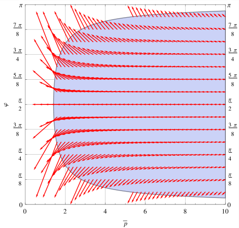
Figure 2: Visualization of the $(\overline{p},\varphi)$ bias correction field of Eq. 9. The tail of each arrow is located at a measured $(\overline{p},\varphi)$ point and the head is attached to the corresponding “Most Probable” estimate of $(\overline{p}_{0},\varphi_{0})$. This correction should only be applied to $(\overline{p},\varphi)$ points lying in the blue region given by Eq. 10. See the text for discussion about $(\overline{p},\varphi)$ points outside the blue region.

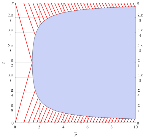
Figure 3: Behavior of the bias correction field (Eq. 9) on the boundary of the blue valid region (Eq. 10). The left-most point on the boundary of the blue region is at $(\sqrt{2},\pi/2)$.

The “bias correction field” in Fig. 2 shows that the correction applied to $\overline{p}$ gets larger as $\overline{p}$ gets smaller (the actual magnitude is $\varphi$-dependent). This is consistent with the known behavior in the two-dimensional case. Fig. 2 also shows that $\varphi$ itself must be corrected: it should be made larger when $\varphi>\pi/2$ and smaller when $\varphi<\pi/2$. The magnitude of this correction also tends to be larger as $\overline{p}$ gets smaller. The exact magnitude of the $\varphi$-correction at a given $\overline{p}$ depends on $\varphi$ itself with the magnitude being largest in the “mid-latitudes” of the Poincaré sphere and zero on the equator. Generally, $(\overline{p},\varphi)$-points not on the equator are “attracted” towards the poles, an effect most prominent at low signal-to-noise (between, say, $\sqrt{2}<\overline{p}\lesssim 5$). The bias correction vector field diminishes as $\overline{p}$ gets larger but for $\varphi$ values near the poles is seen to remain significant even for $\overline{p}>10$, a regime typically thought of as having signal-to-noise high enough not to have to worry about such effects.

For points infinitesimally close to the boundary defined by Eq. 10, the bias correction for $\varphi$ estimates $\varphi_{0}=0$ or $\varphi_{0}=\pi$, whichever pole is nearest. Fig. 3 illustrates this behavior. The special case of $\varphi=\pi/2$ “corrects” to $\varphi_{0}=\pi/2$. More specifically, points on the boundary with $\pi/2<\varphi<\pi$ all bias correct to $\varphi_{0}=\pi$ while those with $0<\varphi<\pi/2$ all bias correct to $\varphi_{0}=0$. The $\overline{p}$ correction on the boundary acts typically and corrects more and more towards the origin as $\overline{p}$ gets smaller.

From Figs. 2 and 3, it can be seen that every possible $(\overline{p}_{0},\varphi_{0})$ with $\overline{p}_{0}>0$ and $\sin\varphi_{0}\neq 0$ is associated with a $(\overline{p},\varphi)$ point within the blue region and vice versa. Unfortunately, a closed form solution for the inverse of Eq. 9 was not found and may not exist.

Intuitively, the $\overline{p}$ correction may be understood by considering a $\overline{p}_{0}$ value of zero. The measured value of $\overline{p}$ cannot be negative and, due to scatter from measurement error, you expect that $\overline{p}$ will almost always be positive (that is, there is a negligibly small chance of zero) even though $\overline{p}_{0}=0$. Thus, the measurement process “biases” $\overline{p}$ to larger values by some amount. Therefore, a correction should be made that subtracts a bit from the measured value to obtain a good estimate of $\overline{p}_{0}$. Even for a non-zero $\overline{p}_{0}$, this biasing occurs although with diminishing effect as $\overline{p}_{0}$ gets larger. The same line of reasoning can be used to gain an intuitive understanding of the $\varphi$ bias correction. Consider a source in a state of pure circular polarization. This corresponds to a pole of the Poincaré sphere. Let’s focus on the purely right-circularly polarized case ($\varphi_{0}=0$). Measurements of this state will be clustered around the pole (including outside the Poincaré sphere) but $\varphi$ is never negative and is almost always positive. Similarly for the left-circularly polarized case ($\varphi_{0}=\pi$), measurements of $\varphi$ will be clustered near that pole but cannot have $\varphi$ greater than $\pi$ and almost always will have $\varphi$ less than $\pi$. Just as with $\overline{p}$, a correction is needed to remove this effect from $\varphi$. It is important to remark that both the $\overline{p}$ and $\varphi$ bias corrections are purely coordinate effects. It may seem at first as if the $\varphi$-correction is inconsistent with the symmetry of the system (from $\Sigma_{Q}=\Sigma_{U}=\Sigma_{V}$) but it is not. While conventionally the $v$-axis is always chosen to isolate circular polarization, the effect would arise regardless of the orientation of the $v$-axis within the Poincaré sphere, which preserves the overall symmetry (i.e., the symmetry is spontaneously broken by introduction of the coordinate system).

It must be stressed that the solution of Eq. 9 only applies to measured points satisfying Eq. 10 (illustrated by the blue region in the figures). Presumably, the area outside the blue region divides into three other regions: one characterized by $\overline{p}_{0,MP}=0$, another by $\overline{p}_{0,MP}\neq 0$ and $\varphi_{0,MP}=0$, and still another by $\overline{p}_{0,MP}\neq 0$ and $\varphi_{0,MP}=\pi$. In the latter two cases, there could still be a $\overline{p}$ bias correction at work. It is unclear how to determine mathematically a “MP solution” in the non-blue region of Fig. 2. A formal solution may simply not exist there. The authors’ best guess as to the best practice is that measurements within the “triangle” defined by points $(0,0)$, $(0,\pi)$, and $(\sqrt{2},\pi/2)$ correct to $(0,\pi)$ if $\varphi>\pi/2$, $(0,0)$ if $\varphi<\pi/2$, and $(0,\pi/2)$ if $\varphi=\pi/2$. The remaining points could correct to the same value as the blue region boundary point whose “correction arrow” passes through the point. Another possibility for these later points is to translate the correction arrow from the boundary of the blue region with the same $\varphi$ to the point and use the intersection of that arrow with the $\overline{p}$-axis as the corrected value. Formal solutions in these regions where not, however, found.

Eq. 9 does indeed provide an estimate of the $(\overline{p}_{0},\varphi_{0})$ point that would produce a distribution of measured points with maximum at $(\overline{p},\varphi)$. It is however just a point estimate. The actual $(\overline{p},\varphi)$ distribution for a small values of $\overline{p}_{0}$ tends to be broad, shallow, and nearly flat, especially in the $\varphi$ dimension. In other words, the errors bars associated with each estimate will be large so it is cautioned that the point estimate should not be taken too literally. Using the $\overline{f}^{\prime}$ distribution, one could construct confidence regions. These regions are however not uniquely determined, even in the one-dimensional case (Simmons & Stewart, 1985). Construction of confidence regions is reserved for future work.

4 Marginalized distributions

Experimenters often work with only a partial description of a physical system. This may be necessary when independent variables of a distribution of interest related to the system are not measurable, or desired when there are so-called nuisance variables of little concern. In a polarization study, for instance, it may be that only the degree of linear polarization is the focus and not the angle of linear polarization. In such situations, one can marginalize over “unwanted” independent variables to find a new distribution which no longer depends on them but at the cost of losing some information present in the original distribution.

The marginalization possibilities for $f^{\prime}$ are to marginalize over (I) $p$only; (II) $\theta$only; (III) $\varphi$only; (IV) $p$and $\theta$; (V) $p$and $\varphi$; and (VI) $\theta$and $\varphi$. The first and last cases are perhaps the most interesting and shall now be investigated.

4.1 The $p$-marginalized angular distribution

The $p$-marginalized angular distribution is

$$M(\theta,\varphi|p_{0},\theta_{0},\varphi_{0},\sigma)=\int_{0}^{\infty}f^{\prime}(p,\theta,\varphi|p_{0},\theta_{0},\varphi_{0},\sigma)\,dp$$ (11)

or, in signal-to-noise variables,

$$\overline{M}(\theta,\varphi|\overline{p}_{0},\theta_{0},\varphi_{0},\sigma)=\int_{0}^{\infty}\overline{f}^{\prime}(\overline{p},\theta,\varphi|\overline{p}_{0},\theta_{0},\varphi_{0},\sigma)\,d\overline{p}.$$ (12)

This equation can be simplified. Start with

$$\overline{M} (\theta,\varphi|\overline{p}_{0},\theta_{0},\varphi_{0},\sigma)$$

$$= \int_{0}^{\infty}\frac{\overline{p}^{2}\sin\varphi}{(2\pi)^{3/2}}e^{-\frac{\overline{p}^{2}+\overline{p}_{0}^{2}-2\overline{p}\,\overline{p}_{0}\left(\sin\varphi\sin\varphi_{0}\cos(\theta-\theta_{0})+\cos\varphi\cos\varphi_{0}\right)}{2}}d\overline{p}$$

$$= \frac{\sin\varphi}{(2\pi)^{3/2}}e^{-\frac{\overline{p}_{0}^{2}}{2}}\int_{0}^{\infty}\overline{p}^{2}e^{-\frac{\overline{p}^{2}-2\overline{p}\,\overline{p}_{0}\left(\sin\varphi\sin\varphi_{0}\cos(\theta-\theta_{0})+\cos\varphi\cos\varphi_{0}\right)}{2}}d\overline{p}$$

and use the definite integral

$$\int_{0}^{\infty}\!x^{2}e^{-\frac{x^{2}+ax}{2}}dx=\sqrt{\frac{\pi}{32}}(a^{2}+4)e^{a^{2}/8}\operatorname{erfc}\left(\frac{a}{2\sqrt{2}}\right)-\frac{a}{2},$$ (13)

where $\operatorname{erfc}(x)$ is the complementary error function defined as

$$\operatorname{erfc}(x)\equiv 1-\operatorname{erf}(x)=\frac{2}{\sqrt{\pi}}\int_{x}^{\infty}e^{-t^{2}}dt$$ (14)

and $\operatorname{erf}(x)$ is the error function to reduce this integral.

$$\overline{M}(\theta,\varphi|\overline{p}_{0},\theta_{0},\varphi_{0},{} \sigma)=$$ (15)

$$\frac{\sin\varphi}{(2\pi)^{3/2}}e^{-\frac{\overline{p}_{0}^{2}}{2}} \left(\sqrt{\frac{\pi}{32}}(A^{2}+4)e^{A^{2}/8}\operatorname{erfc}\left(\frac{A}{2\sqrt{2}}\right)-\frac{A}{2}\right)$$

is obtained where

$$A\equiv-2\,\overline{p}_{0}\left(\sin\varphi\sin\varphi_{0}\cos(\theta-\theta_{0})+\cos\varphi\cos\varphi_{0}\right)$$ (16)

which may be viewed as a higher-dimensional analog of the angular distribution presented in Vinokur (1965) (see also Clarke & Stewart (1986); Naghizadeh-Khouei & Clarke (1993); Quinn (2012)).

Examining a few density plots of Eq. 15 for various values of $\overline{p}_{0}$, $\theta_{0}$, and $\varphi_{0}$ reveals that the probability distribution is attenuated near the poles of the coordinate system, an effect that becomes broader for small values of $\overline{p}_{0}$. In particular, one should notice that even for $\overline{p}_{0}=0$, the probability density still varies with $\varphi$. This is due to the pole bias effect discussed earlier.

One would like to go further and find the two one-dimensional marginalized angular distributions (cases IV and V) but the integrations seem unable to be completely performed using elementary or even common special functions.

4.2 The angular-marginalized $p$-distribution

One is often primarily concerned with the degree of polarization, $p$, and not the value of the angular variables. Marginalization over the angular variables will therefore produce a new distribution, to be called $\mathscr{Q}$ ($\overline{\mathscr{Q}}$ in signal-to-noise variables) of high practical importance. In the polar coordinate case, marginalization over the (lone) angular variable, $\theta$, produces the Rice distribution. In the spherical coordinate case, the marginalization must occur over both $\theta$ and $\varphi$. Thus, the function $\overline{\mathscr{Q}}$ may be considered a higher-dimensional analog of the Rice distribution. Let

$$\mathscr{Q}(p|p_{0},\theta_{0},\varphi_{0},\sigma)=\int_{0}^{\pi}\!\int_{-\pi}^{\pi}f^{\prime}(p,\theta,\varphi|p_{0},\theta_{0},\varphi_{0},\sigma)\,d\theta\,d\varphi$$ (17)

or similarly

$$\overline{\mathscr{Q}}(\overline{p}|\overline{p}_{0},\theta_{0},\varphi_{0},\sigma)=\int_{0}^{\pi}\!\int_{-\pi}^{\pi}\overline{f}^{\prime}(\overline{p},\theta,\varphi|\overline{p}_{0},\theta_{0},\varphi_{0},\sigma)\,d\theta\,d\varphi.$$ (18)

Let’s calculate.

$$\begin{aligned} \overline{\mathscr{Q}}{}&(\overline{p}|\overline{p}_{0},\theta_{0},\varphi_{0},\sigma)=\frac{\overline{p}^{2}}{(2\pi)^{3/2}}e^{-\frac{\overline{p}^{2}+\overline{p}_{0}^{2}}{2}}\times\\ &\int_{0}^{\pi}\!\int_{-\pi}^{\pi}\!\sin\varphi\,e^{\overline{p}\,\overline{p}_{0}(\sin\varphi\sin\varphi_{0}\cos(\theta-\theta_{0})+\cos\varphi\cos\varphi_{0})}\,d\theta\,d\varphi\\ ={}&\frac{\overline{p}^{2}}{(2\pi)^{3/2}}e^{-\frac{\overline{p}^{2}+\overline{p}_{0}^{2}}{2}}\times\\ &\int_{0}^{\pi}\!\sin\varphi\,e^{\overline{p}\,\overline{p}_{0}\cos\varphi\cos\varphi_{0}}\int_{-\pi}^{\pi}\!e^{\overline{p}\,\overline{p}_{0}\sin\varphi\sin\varphi_{0}\cos(\theta-\theta_{0})}\,d\theta\,d\varphi\end{aligned}$$ (19)

The $\theta$-integral can be solved using $\int_{-\pi}^{\pi}e^{a\cos(t)}dt=2\pi\mathcal{I}_{0}(a)$, where $\mathcal{I}_{0}(x)$ is the modified Bessel function of the first kind. $\mathcal{I}_{0}$ is an even, real function when its argument is real. (Because the range of integration is over a full period of $\theta$, the value of $\theta_{0}$ is immaterial because it appears as a phase shift and does not affect the integral.) Once the $\theta$-integral is performed, the $\overline{\mathscr{Q}}$ distribution no longer explicitly depends on $\theta_{0}$. We shall therefore drop $\theta_{0}$ from the conditions. Continuing with the calculation,

$$\begin{aligned} \overline{\mathscr{Q}}(\overline{p}|&\overline{p}_{0},\varphi_{0},\sigma)=\frac{\overline{p}^{2}}{(2\pi)^{3/2}}e^{-\frac{\overline{p}^{2}+\overline{p}_{0}^{2}}{2}}\times\\ &\int_{0}^{\pi}\!\sin\varphi\,e^{\overline{p}\,\overline{p}_{0}\cos\varphi\cos\varphi_{0}}(2\pi)\mathcal{I}_{0}(\overline{p}\,\overline{p}_{0}\sin\varphi\sin\varphi_{0})d\varphi\\ ={}&\frac{\overline{p}^{2}}{\sqrt{2\pi}}e^{-\frac{\overline{p}^{2}+\overline{p}_{0}^{2}}{2}}\times\\ &\int_{0}^{\pi}\!\sin\varphi\,e^{\overline{p}\,\overline{p}_{0}\cos\varphi\cos\varphi_{0}}\mathcal{I}_{0}(\overline{p}\,\overline{p}_{0}\sin\varphi\sin\varphi_{0})d\varphi.\end{aligned}$$ (20)

The $\varphi$-integral in the last expression is non-trivial but it appears it can be solved. Let

$$\omega(a,\varphi,\varphi_{0})\equiv\sin\varphi\,e^{a\cos\varphi\cos\varphi_{0}}\mathcal{I}_{0}(a\sin\varphi\sin\varphi_{0})$$ (21)

and

$$\Omega(a,\varphi_{0})\equiv\int_{0}^{\pi}\!\omega(a,\varphi,\varphi_{0})d\varphi,$$ (22)

where $a\equiv\overline{p}\,\overline{p}_{0}\geq 0$. No computer algebra system tested could solve the integral in Eq. 22 and no applicable integrals were found in tables of integrals. Manual attempts to solve it also failed. From graphs of $\Omega$ versus $\varphi_{0}$ created numerically for several values of $a$, it is noticed that the function may actually be constant in $\varphi_{0}$ for a given $a$. Unfortunately, it is not a simple matter to show $\frac{\partial\Omega}{\partial\varphi_{0}}=0$ but if $\frac{\partial\Omega}{\partial\varphi_{0}}$ is graphed for $0\leq\varphi_{0}\leq\pi$ at several sampled values of $a$ it seems to always show residuals about zero with scatter consistent with numerical noise. The previous numerical observations lead one to suspect very strongly that $\Omega(a,\varphi_{0})$ is independent of the value of $\varphi_{0}$. This may be surprising in light of the bias corrections previously discussed; however, the same marginalized formula seems like it should be found regardless of the rotational orientation of the $(\overline{q},\overline{u},\overline{v})$ coordinate system within the Poincaré sphere. If it is true that $\Omega(a,\varphi_{0})$ is constant in $\varphi_{0}$, any value of $\varphi_{0}$ may be chosen and it does not alter $\Omega(a,\varphi_{0})$’s value at a given $a$. In that case, a value of $\varphi_{0}$ may be judiciously chosen that simplifies the integral. Good choices are $\varphi_{0}=0$ or $\pi$ for which

$$\Omega(a,\varphi_{0})=\frac{2\sinh(a)}{a}$$ (23)

is found using the common integral $\int_{0}^{\pi}\!e^{x\cos{\varphi}}\sin{\varphi}\,d\varphi=2\sinh(x)/x$, where $\sinh(x)$ is the hyperbolic sine of $x$. Indeed, simple arguments modifying the factors in the integrand of Eq. 22 can prove this to be a lower limit for $\Omega(a,\varphi_{0})$ at a given $a$ (see Appendix A). Proof that it is also the upper limit was elusive (except at $\varphi_{0}=0$, $\pi/2$, and $\pi$). A Taylor series expansion of $\Omega(a,\varphi_{0})$ in $\varphi_{0}$ at $\varphi_{0}=0$ was found to be consistent with Eq. 23 out to 26-th order using computer algebra systems. Based on physical suspicion corroborated by numerical results, Eq. 23 shall be assumed to be true henceforth.

Returning to the main distribution and using Eq. 23, $\overline{\mathscr{Q}}$, it is proposed that

$$\overline{\mathscr{Q}}(\overline{p}|\overline{p}_{0},\sigma)=\sqrt{\frac{2}{\pi}}\frac{\overline{p}}{\overline{p}_{0}}e^{-\frac{\overline{p}^{2}+\overline{p}_{0}^{2}}{2}}\sinh(\overline{p}\,\overline{p}_{0}).$$ (24)

Since the value of $\varphi_{0}$ is irrelevant, $\overline{\mathscr{Q}}$’s dependence on $\varphi_{0}$ has been dropped from the notation. This is the higher-dimensional analog of the Rice distribution. Surprisingly, it is a simpler function than the Rice distribution in the sense that it depends on the hyperbolic sine function rather than a modified Bessel function. The $\overline{\mathscr{Q}}$ distribution is normalized, $\int_{0}^{\infty}\!\overline{\mathscr{Q}}\,d\overline{p}=1$.

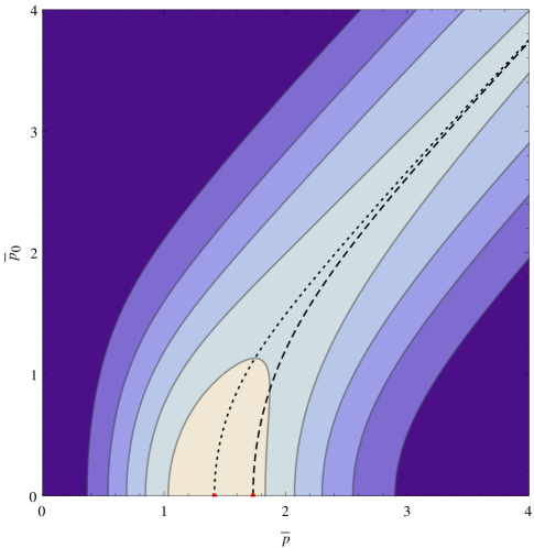
Figure 4: Contour plot of the angular-marginalized $\overline{p}$-distribution given by Eq. 24. The contours are at $0.1$ intervals with the lighter shades corresponding to larger values. The dotted and dashed curves (Eqs. 25 and 26) trace maximums along horizontal and vertical slices and end at the red points at $(\sqrt{2},0)$ and $(\sqrt{3},0)$, respectively. Although the “shape” of the distribution is not affected by the value of $\sigma$, the plot assumes that $\sigma\leq 1/4$ so that the plotted values for $\overline{p}_{0}$ up to $4$ ($=1/\sigma_{max}$) exist.

Some general properties of $\overline{\mathscr{Q}}$ can now be investigated. A contour plot of the function is shown in Fig. 4 with contours at $0.1$ intervals. The function achieves a global maximum as $(\overline{p},\overline{p}_{0})$ approaches $(\sqrt{2},0)$ of $\frac{2}{e}\sqrt{\frac{2}{\pi}}\approx 0.587051$. Tracing the maximums of horizontal slices (the dotted line in the figure) yields the equation $(\overline{p}^{2}-1)\sinh(\overline{p}\,\overline{p}_{0})-\overline{p}\,\overline{p}_{0}\cosh(\overline{p}\,\overline{p}_{0})=0$ or

$$(\overline{p}_{0}^{2}-1)\tanh(\overline{p}\,\overline{p}_{0})=\overline{p}\,\overline{p}_{0}$$ (25)

This implicit curve intersects the $\overline{p}$-axis at the global maximum at $(\sqrt{2},0)$ and is the “Most Probable” estimator curve for $\overline{\mathscr{Q}}$. Tracing the maximums of vertical slices (dashed line) yields $\overline{p}\,\overline{p}_{0}\cosh(\overline{p}\,\overline{p}_{0})-(\overline{p}_{0}^{2}+1)\sinh(\overline{p}\,\overline{p}_{0})=0$ or

$$(\overline{p}_{0}^{2}+1)\tanh(\overline{p}\,\overline{p}_{0})=\overline{p}\,\overline{p}_{0}$$ (26)

This curve intersects at the $\overline{p}$-axis at $(\sqrt{3},0)$ and is the “Most Likely” estimator curve for $\overline{\mathscr{Q}}$.

The MP estimator curve of Eq. 25 (dotted curve in Fig. 4) can be used for all $\overline{p}>\sqrt{2}$. Yet it was stressed that the full MP solution given Eqs. 9 and 10 is only valid for some values with $\overline{p}>\sqrt{2}$. Marginalization has thus hidden some of the complexity of the problem. The ML estimator given by Eq. 26 (dashed curve) now has non-trivial behavior unlike the full solution in Eq. 8. It is not easy to anticipate the effect that marginalization will have on various estimators.

It is interesting to compare the long form of these estimator curves and the corresponding curves based on the Rice distribution (Wardle & Kronberg, 1974; Simmons & Stewart, 1985; Quinn, 2012). These curves are based on the hyperbolic trigonometric functions whereas the curves in the two-dimensional case are based on Bessel functions. Their points of intersection with the $\overline{p}$-axis have also been shifted by $1$. The differences arise because the Jacobian factor is proportional to $p^{2}$ in spherical coordinates but only $p$ for polar coordinates.

5 Discussion

How do these new results relate to the old results derived using polar coordinates for the “Poincaré disk”? First, the old results are not special cases of the new results when $\varphi\rightarrow\pi/2$ and $\varphi_{0}\rightarrow\pi/2$; for instance, in the special case of $\varphi=\pi/2$, the $\overline{p}$ equation of Eq. 9 reduces to $\overline{p}-2/\overline{p}$ rather than the Wang estimator $\overline{p}-1/\overline{p}$ (Wang et al., 1997; Quinn, 2012) and $\overline{M}(\theta,\varphi)$ does not reduce to angular distribution given by Vinokur (1965). Similarly, $\overline{\mathscr{Q}}$ is altogether distinct from the Rice distribution. The new results are therefore not direct extensions of the old functions but they do have somewhat similar forms. The three versus two dimensional nature of the parameter space is responsible for this.

Particularly interesting is a comparison of Fig. 4 with fig. 2a of Quinn (2012). The intercepts of all the estimator curves have undergone shifts of the form $\sqrt{n}\rightarrow\sqrt{n+1}$. This again is due to the increased dimensionality of the problem. Thus, when circular polarization has equal measurement error to the linear Stokes axes’ measurement error, it takes a bigger measurement of the magnitude of the polarization vector to be significant than the two-dimensional case suggests. The two-dimensional results can perhaps be recovered by some limiting procedure where $\sigma_{v}\rightarrow 0$ while $\sigma$ ($=\sigma_{q}=\sigma_{u}$) is held constant. This suggests that decreasing the measurement error on one of $\sigma_{q}$, $\sigma_{u}$, or $\sigma_{v}$ should decrease the $\overline{p}$-threshold for a significant measurement. On the other hand, often an instrument measures only linear or only circular polarization. This may correspond to a scenario where the distribution of Stokes parameters is best modeled by assuming a flat (instead of gaussian) distribution for the variables of the undetected type. This would violate our starting assumptions in Eq. 1 and would produce rather different results. As a flat distribution is in an informal sense a “wide” distribution, it is probable that this would raise the detection threshold higher. It should be clear that interpreting polarization data at low signal-to-noise in “human digestible” quantities like degrees of polarization or angle of polarization is difficult.

6 Conclusion

The three-dimensional Stokes sampling distribution in spherical coordinates is given. From it the “Most Likely” and “Most Probable” classical (that is, non-Bayesian) estimators for the “true” Stokes parameters given measured values have been derived. Additionally, a two useful marginalizations of the sampling distribution have been calculated including a higher dimensional analog of the Rice distribution. These results are necessary stepping stones towards a full and proper treatment of polarization measurements.

It is cautioned that a deep understanding of the measurement of Stokes parameters in spherical coordinates like here or the polar coordinates usually used for linear polarization requires a Bayesian approach. The presented results may nonetheless have tolerable accuracy for many experiments.

While the setup of the problem and the presentation of the results has been framed in terms of the study of polarization, the solutions are in fact far more general. They are applicable to the measurement of any “source point” contained in a three-dimensional ball measured with Gaussian error in each Cartesian direction and presented in spherical coordinates. The results could be used to study the location of neutrino production within the Sun or the determination of the epicenter of an earthquake. The results could also influence the interpretation of cosmic microwave background polarization data. Extensions of the work removing the constraint that the error be equal in each direction or that involve correlated variables would be highly desirable.

Appendix A Bounds on $\Omega(a,\varphi_{0})$

It helps to have functional bounds on

$$\Omega(a,\varphi_{0})\equiv\int_{0}^{\pi}\!\sin(\varphi)e^{a\cos(\varphi)\cos(\varphi_{0})}I_{0}(a\sin(\varphi)\sin(\varphi_{0}))\,d\varphi$$ (27)

to show, for instance, that it is at least non-infinite over the $\varphi_{0}$-domain of interest. There are three factors ($\sin(\varphi)$, $e^{a\cos(\varphi)\cos(\varphi_{0})}$, and $I_{0}(a\sin(\varphi)\sin(\varphi_{0}))$) in the integrand, each of which is simple enough that they allow various bounds to be obtained for the total expression.

A.1 Lower bound

Under variation of $\varphi_{0}$, the $e^{a\cos(\varphi)\cos(\varphi_{0})}$ factor is minimized when $\cos(\varphi_{0})$ is the smallest, which occurs for $\varphi_{0}=\pi$, so that the factor becomes $e^{-a\cos(\varphi)}$. Furthermore, the $I_{0}(a\sin(\varphi)\sin(\varphi_{0}))$ factor is the smallest when its argument is zero, which also occurs at $\varphi_{0}=\pi$ (also $\varphi_{0}=0$) so that the factor become $\mathcal{I}_{0}(0)=1$. After these substitutions, the integral for $\Omega$ can be performed explicitly:

$$\int_{0}^{\pi}\!\sin(\varphi)\,e^{-a\cos(\varphi)}d\varphi=\frac{2\sinh(a)}{a}.$$ (28)

For any given value of $a$, this sets a (constant) global lower bound on the integral: the value of integral must be greater than or equal to $\frac{2\sinh(a)}{a}$ for all values of $\varphi_{0}$. It is probably also the greatest lower bound for each $\varphi_{0}$.

A.2 Upper bounds

The $e^{a\cos(\varphi)\cos(\varphi_{0})}$ factor is maximized when its exponent is the largest while the $I_{0}(a\sin(\varphi)\sin(\varphi_{0}))$ factor is the largest when the magnitude of its argument is as big as possible.

A constant global upper bound is found by modifying the factors in the obvious way:

$$\int_{0}^{\pi}\!\sin(\varphi)\,e^{a\cos(\varphi)}\mathcal{I}_{0}(\pm a)\,d\varphi=\frac{2\sinh(a)}{a}\mathcal{I}_{0}(a).$$ (29)

A stricter (but non-constant) global upper bound can be found merely by allowing $\sin(\varphi_{0})\rightarrow 1$ in the Bessel function factor,

$$\int_{0}^{\pi}\!\sin(\varphi) \,e^{a\cos(\varphi)\cos(\varphi_{0})}\mathcal{I}_{0}(a\sin(\varphi))\,d\varphi$$ (30)

$$=\frac{2\sec(\varphi_{0})\sinh(a\cos(\varphi_{0}))}{a}\mathcal{I}_{0}(a)\quad\quad\text{for }\varphi_{0}\neq\pi/2.$$

This last solution has functional dependence on $\varphi_{0}$ and is not valid for $\varphi_{0}=\pi/2$ because of the $\sec(\varphi_{0})$ component. For $\varphi_{0}=0$ this bound is $\frac{2\sinh(a)}{a}\mathcal{I}_{0}(a)$ and it decreases smoothly and approaches $\frac{2\sinh(a)}{a}$ as $\varphi_{0}\rightarrow\pi/2^{+}$. Similarly, for $\varphi_{0}=\pi$ it is $\frac{2\sinh(a)}{a}\mathcal{I}_{0}(a)$ and it decreases smoothly and approaches $\frac{2\sinh(a)}{a}$ as $\varphi_{0}\rightarrow\pi/2^{-}$. Of course, if $\varphi_{0}=\pi/2$, Eq. 27 can be accomplished directly:

$$\int_{0}^{\pi}\sin(\varphi)\,e^{0}\mathcal{I}_{0}(a\sin(\varphi))\,d\varphi=\frac{2\sinh(a)}{a}\quad\text{for }\varphi_{0}=\pi/2,$$ (31)

so the discontinuity in Eq. 30 at $\varphi_{0}=\pi/2$ can be “removed”. Eq. 27 can also be performed for $\varphi_{0}=0$ and $\varphi_{0}=\pi$ and in both cases $\frac{2\sinh(a)}{a}$ results, so we have explicit upper bounds at those values too.

A.3 Best bounds

Combining the previous information, the best bounds are

$$\frac{2\sinh(a)}{a}\leq\Omega(a,\varphi_{0})\leq\begin{cases}\frac{2\sinh(a)}{a}&\mbox{if }\varphi_{0}=0,\frac{\pi}{2},\pi\\ \frac{2\sec(\varphi_{0})\sinh(a\cos(\varphi_{0}))}{a}\mathcal{I}_{0}(a)&\mbox{otherwise,}\end{cases}$$ (32)

which are finite for all $\varphi_{0}$ at a given value of $a$.

References

- Ade et al. (2014a) Ade, P. A. R., Aikin, R. W., Amiri, M., et al. 2014a, ApJ, 792, 62
- Ade et al. (2014b) Ade, P. A. R., Aikin, R. W., Barkats, D., et al. 2014b, Physical Review Letters, 112, 241101
- Clarke & Stewart (1986) Clarke, D. & Stewart, B. G. 1986, Vistas in Astronomy, 29, 27
- del Toro Iniesta (2003) del Toro Iniesta, J. C. 2003, Introduction to Spectropolarimetry (Cambridge University Press)
- Kuo & BICEP3 and POLAR1 Collaborations (2013) Kuo, C.-L. & BICEP3 and POLAR1 Collaborations. 2013, in IAU Symposium, Vol. 288, IAU Symposium, ed. M. G. Burton, X. Cui, & N. F. H. Tothill, 80–83
- Landi Degl’Innocenti (2002) Landi Degl’Innocenti, E. 2002, in Astrophysical Spectropolarimetry, ed. J. Trujillo-Bueno, F. Moreno-Insertis, & F. Sánchez, 1–53
- Leonard et al. (2005) Leonard, D. C., Li, W., Filippenko, A. V., Foley, R. J., & Chornock, R. 2005, ApJ, 632, 450
- Liu et al. (2014) Liu, H., Mertsch, P., & Sarkar, S. 2014, ApJ, 789, L29
- Maeda et al. (2011) Maeda, K., Leloudas, G., Taubenberger, S., et al. 2011, MNRAS, 413, 3075
- Mauerhan et al. (2014) Mauerhan, J., Williams, G. G., Smith, N., et al. 2014, MNRAS, 442, 1166
- Maund et al. (2010a) Maund, J. R., Höflich, P., Patat, F., et al. 2010a, ApJ, 725, L167
- Maund et al. (2013) Maund, J. R., Spyromilio, J., Höflich, P. A., et al. 2013, MNRAS, 433, L20
- Maund et al. (2010b) Maund, J. R., Wheeler, J. C., Wang, L., et al. 2010b, ApJ, 722, 1162
- Montier et al. (2014a) Montier, L., Plaszczynski, S., Levrier, F., et al. 2014a, ArXiv e-prints 1406.6536
- Montier et al. (2014b) Montier, L., Plaszczynski, S., Levrier, F., et al. 2014b, ArXiv e-prints 1407.0178
- Naghizadeh-Khouei & Clarke (1993) Naghizadeh-Khouei, J. & Clarke, D. 1993, A&A, 274, 968
- Patat et al. (2012) Patat, F., Höflich, P., Baade, D., et al. 2012, A&A, 545, A7
- Perlmutter et al. (1999) Perlmutter, S., Aldering, G., Goldhaber, G., et al. 1999, ApJ, 517, 565
- Planck Collaboration (2014) Planck Collaboration. 2014, ArXiv e-prints 1405.0871
- Quinn (2012) Quinn, J. L. 2012, A&A, 538, A65
- Rice (1945) Rice, S. O. 1945, Bell Systems Tech. J., Volume 24, p. 46-156, 24, 46
- Riess et al. (1998) Riess, A. G., Filippenko, A. V., Challis, P., et al. 1998, AJ, 116, 1009
- Simmons & Stewart (1985) Simmons, J. F. L. & Stewart, B. G. 1985, A&A, 142, 100
- Staniszewski et al. (2012) Staniszewski, Z., Aikin, R. W., Amiri, M., et al. 2012, Journal of Low Temperature Physics, 167, 827
- Stokes (1852) Stokes, G. G. 1852, Trans. Cambridge Phil. Soc., 9, 399
- Tanaka et al. (2012) Tanaka, M., Kawabata, K. S., Hattori, T., et al. 2012, ApJ, 754, 63
- The POLARBEAR Collaboration (2014) The POLARBEAR Collaboration. 2014, ArXiv e-prints 1403.2369
- Vaillancourt (2006) Vaillancourt, J. E. 2006, PASP, 118, 1340
- Vinokur (1965) Vinokur, M. 1965, Annales d’Astrophysique, 28, 412
- Wang et al. (2007) Wang, L., Baade, D., & Patat, F. 2007, Science, 315, 212
- Wang & Wheeler (2008) Wang, L. & Wheeler, J. C. 2008, ARA&A, 46, 433
- Wang et al. (1997) Wang, L., Wheeler, J. C., & Hoeflich, P. 1997, ApJ, 476, L27+
- Wang et al. (2013) Wang, X., Wang, L., Filippenko, A. V., Zhang, T., & Zhao, X. 2013, Science, 340, 170
- Wardle & Kronberg (1974) Wardle, J. F. C. & Kronberg, P. P. 1974, ApJ, 194, 249
- Zelaya et al. (2013) Zelaya, P., Quinn, J. R., Baade, D., et al. 2013, AJ, 145, 27