Concentration dependence of the Flory-Huggins interaction parameter in aqueous solutions of capped PEO chains

Abstract

The dependence on volume fraction $\varphi$ of the Flory-Huggins $\chi_{\mathrm{wp}}\left(\varphi\right)$ describing the free energy of mixing of polymers in water is obtained by exploiting the connection of $\chi_{\mathrm{wp}}\left(\varphi\right)$ to the chemical potential of the water, for which quasi-chemical theory is satisfactory. We test this theoretical approach with simulation data for aqueous solutions of capped PEO oligomers. For CH₃(CH₂-O-CH₂)_mCH₃ ($m$=11), $\chi_{\mathrm{wp}}\left(\varphi\right)$ depends strongly on $\varphi$, consistent with experiment. These results identify coexisting water-rich and water-poor solutions at $T$ = 300 K and $p$ = 1 atm. Direct observation of the coexistence of these two solutions on simulation time scales supports that prediction for the system studied. This approach directly provides the osmotic pressures. The osmotic second virial coefficient for these chains is positive, reflecting repulsive interactions between the chains in the water, a good solvent for these chains.

I Introduction

A classic element of polymer solution physics, the Flory-Huggins (FH) model,Flory (1953); Huggins (1941)

$$\frac{\beta\Delta{G_{\mathrm{mix}}}}{n_{\mathrm{w}}+Mn_{\mathrm{p}}}=\varphi\ln\varphi+\frac{\left(1-\varphi\right)}{M}\ln\left(1-\varphi\right)\\ +\varphi\left(1-\varphi\right)\chi_{\mathrm{wp}}~{},$$ (1.1)

describes the free energy of mixing of $n_{\mathrm{p}}$ moles of polymer liquid with $n_{\mathrm{w}}$ moles of the water solvent; $\beta=1/kT$, $\varphi$ is the solvent volume fraction, $M=\bar{v}_{\mathrm{p}}/\bar{v}_{\mathrm{w}}$ (the ratio of the molar volumes of the pure liquids) is the operational polymerization index, and $\chi_{\mathrm{wp}}$ is the FH interaction coefficient. Here we study the concentration dependence of $\chi_{\mathrm{wp}}$, important for mixing the dissimilar liquids of water and chain molecules that have a non-trivial aqueous solubility. The FH model is routinely adopted for discussion of aqueous solutions of chain molecules of sub-polymeric length.Sharp et al. (1991); De Young and Dill (1990); Stillinger (1983) The study below highlights direct access to the osmotic pressures of these solutions, and thus can address long-standing research on biophysical hydration forces.Parsegian and Zemb (2011)

Though the traditional statistical mechanical calculationHill (1960) that arrives at Eq. (1.1) is not compelling for aqueous materials, the FH model captures two dominating points. Firstly, it identifies the volume fraction $\varphi$ as the preferred concentration variable, associated with the physical assumption that the excess volume of mixing vanishes. This step partially avoids difficult statistical mechanical packing problems.Beck et al. (2006) Secondly, Eq. (1.1) captures the reduction of the chain molecule ideal entropy by the factor $1/M$. The physical identification of the polymerization index $M$ as $\bar{v}_{\mathrm{p}}/\bar{v}_{\mathrm{w}}$ as thermodynamically consistent as noted below, but is a crude description of the molecular structure of polymers. With these points recognized, however, the interaction contribution of Eq. (1.1) can be regarded as an interpolation between the ends $\varphi=0,1$ of the composition range.

The simplest expectation Hill (1960); Doi (1995); Bae et al. (1993); Beck et al. (2006) for the interaction parameter is

$$\chi_{\mathrm{wp}}\propto-\beta\left(a_{\mathrm{ww}}-\frac{2a_{\mathrm{wp}}}{M}+\frac{a_{\mathrm{pp}}}{M^{2}}\right)$$ (1.2)

where the parameters $a_{\eta\nu}$ gauge the strength of dispersion interactions in van der Waals models of liquids.Chandler et al. (1983) That this justification is implausible for aqueous solutionsShah et al. (2007) underscores the lack of a basic understanding of $\chi_{\mathrm{wp}}$ for aqueous solutions.

The simple temperature dependence of Eq. (1.2) is a reasonable starting point, but aqueous solutions exhibit alternative temperature dependences of specific interest, hydrophobic effects.Pohorille and Pratt (2012) More troublesome, Eq. (1.2) does not depend on concentration, though experiments on the PEG/water system Bae et al. (1993); Eliassi and Modarress (1999) show substantial concentration dependence. Beyond that difficulty, those results exhibit a temperature trend opposite to Eq. (1.2), i.e., stronger interactions at higher $T$  consistent with the classic folklore of hydrophobic effects.Bae et al. (1993) In contrast, when the solvent is methanol Zafarani-Moattar and Tohidifar (2006) the observed concentration dependence is less strong, though non-trivial and trending with concentration in the opposite direction from the aqueous solution results. The temperature dependences for the methanol case is qualitatively consistent with the simple expectation of Eq. (1.2). In further contrast, with ethanol as solvent Zafarani-Moattar and Tohidifar (2008) the observed concentration dependence is distinctly modest.

II Theory

These puzzles may be addressed by analyzing the chemical potential of the water,Bae et al. (1993)

$$\beta\Delta\mu^{\mathrm{(ex)}}_{\mathrm{w}}=\left(1-\frac{1}{M}\right)\left(1-\varphi\right)\\ +\frac{\partial\left(\varphi\chi_{\mathrm{wp}}\right)}{\partial\varphi}\left(1-\varphi\right)^{2}~{},$$ (2.3)

where

$$\Delta\mu^{\mathrm{(ex)}}_{\mathrm{w}}=\mu^{\mathrm{(ex)}}_{\mathrm{w}}\left(\varphi,p,T\right)-\mu^{\mathrm{(ex)}}_{\mathrm{w}}\left(\varphi=1,p,T\right)~{},$$ (2.4)

the interaction (or excess) contribution to the chemical potential of the water, referenced to the pure liquid value. The osmotic pressure $\pi$, Hill (1960)

$$\beta\pi\bar{v}_{\mathrm{w}}=-\ln\varphi-\beta\Delta\mu^{\mathrm{(ex)}}_{\mathrm{w}}~{}.$$ (2.5)

provides further perspective on $\Delta\mu^{\mathrm{(ex)}}_{\mathrm{w}}$. Beyond assuming that the excess volume of mixing vanishes, Eq. (2.5) makes the standard approximation that the solvent is incompressible.Kirkwood and Oppenheim (1961) To justify the identification $M=\bar{v}_{\mathrm{p}}/\bar{v}_{\mathrm{w}}$ noted above, we utilize Eq. (2.3), and expand through $\left(1-\varphi\right)^{2}$ to obtain

$$\beta\pi V/n_{\mathrm{p}}\sim 1+\left(\frac{n_{\mathrm{p}}}{V}\right)\bar{v}_{\mathrm{w}}M^{2}\left(\frac{1}{2}-\hat{\chi}\right)~{},$$ (2.6)

with $\bar{v}_{\mathrm{w}}M^{2}\left(\frac{1}{2}-\hat{\chi}\right)=B_{2}$ thus the osmotic second virial coefficient. We adopt here the short-hand notation $\hat{\chi}=\partial\left(\varphi\chi_{\mathrm{wp}}\right)/\partial\varphi.$ The identification of $M$ in the contribution $\left(1-\varphi\right)\left(1-\frac{1}{M}\right)$ thus leads to the proper behavior in the ideal solution limit.

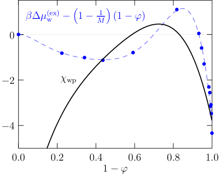
Figure 1: Blue points and dashed curve: accumulated evaluation of Eq. (2.3). The solid curve is the implied $\chi_{\mathrm{WP}}\left(\varphi\right)$.

As suggested above, the intent of the FH model is that a concentration-independent $\chi_{\mathrm{wp}}$ should describe the effects of enthalpic interactions. Our less-committal analysis acquires practical significance from recent development of molecular quasi-chemical theory for the excess chemical potential of the water in aqueous solutions.Shah et al. (2007); Paliwal et al. (2006); Chempath et al. (2009) The central result

$$\beta\mu^{\mathrm{(ex)}}_{\mathrm{w}}\left(\varphi,p,T\right)=-\ln p^{(0)}(n_{\lambda}=0)\\ +\ln\langle{e}^{\beta\varepsilon}\mid{n_{\lambda}=0}\rangle+\ln p(n_{\lambda}=0)$$ (2.7)

is a physical description in terms of packing, outer-shell and chemical contributions, a comprehensive extension of a van der Waals picture.Chandler et al. (1983) The packing contribution is obtained from the observed probability $p^{(0)}(n_{\lambda}=0)$ for successful random insertion of a spherical cavity of radius $\lambda$ into the simulation cell. Similarly, the chemical contribution is defined with the probability $p(n_{\lambda}=0)$ that a water molecule in the system has zero neighbors within the radius $\lambda$ of its O atom. The outer-shell contribution is a partition function involving the binding energy $\varepsilon$, conditional on the inner-shell being empty. The condition permits a Gaussian statistical approximation,

$$\ln\langle{e}^{\beta\varepsilon}\mid{n_{\lambda}=0}\rangle\approx\beta\langle\varepsilon\mid{n_{\lambda}=0}\rangle\\ +\beta^{2}\langle\delta\varepsilon^{2}\mid{n_{\lambda}=0\rangle}/2~{},$$ (2.8)

involving the mean and variance of binding energies of molecules that have zero neighbors within radius $\lambda$.

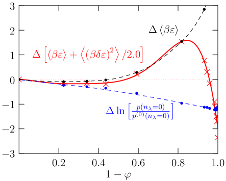
Figure 2: ‘$\Delta$’ indicates the difference from the pure solvent value, i.e., $\Delta\left\langle\beta\varepsilon\right\rangle$ = $\left\langle\beta\varepsilon\right\rangle\left(\varphi\right)$ - $\left\langle\beta\varepsilon\right\rangle\left(\varphi=1\right)$. A water molecule loses stabilizing outer-shell interactions through intermediate concentrations, and then regains favorable outer-shell contributions on the solvent-poor side of the concentration range. The dashed-blue curve shows the combined packing and chemical contributions.

With this background, we evaluate

$$\frac{\partial\left(\varphi\chi_{\mathrm{wp}}\right)}{\partial\varphi}\left(1-\varphi\right)^{2}=\beta\Delta\mu^{\mathrm{(ex)}}_{\mathrm{w}}\\ -\left(1-\frac{1}{M}\right)\left(1-\varphi\right)~{}.$$ (2.9)

Representing then

$$\frac{\partial\left(\varphi\chi_{\mathrm{wp}}\right)}{\partial\varphi}=\sum_{n=0}c_{n}\left(1-\varphi\right)^{n}~{},$$ (2.10)

and integrating, with $\varphi\chi_{\mathrm{wp}}=0$ at $\varphi=0$, we obtain

$$\chi_{\mathrm{wp}}=\sum_{n=0}\frac{c_{n}}{\left(n+1\right)\varphi}\left[1-\left(1-\varphi\right)^{n+1}\right]~{}.$$ (2.11)

III Results and Discussion

We thus analyze $\chi_{\mathrm{WP}}\left(\varphi\right)$ for aqueous solutions for methyl-capped PEO oligomers Chaudhari et al. (2010) CH₃(CH₂-O-CH₂)₁₁CH₃ on the basis of accessible molecular simulation data.Chaudhari (2014) For this mixture we find $M$ = 27.6, with the excess volumes of mixing similar to experimental results for similarly sized PEG 400:Eliassi and Modarress (1999) negative and small, though slightly larger than the comparable experimental case. The dielectric constant of these solution varies linearly with solvent volume fraction $\varphi$.

Eq. (2.7) is correct for any physical $\lambda$, Paliwal et al. (2006) and we choose $\lambda=0.29$ nm as a balance between statistical and systematic accuracy. The Gaussian approximation will be more accurate for larger $\lambda$. But the data set satisfying the condition $n_{\lambda}=0$ gets smaller and the statistical accuracy is degraded with increasing $\lambda$. The latter point becomes more serious at lower water concentrations because fewer water molecules are present. Nevertheless, only the difference Eq. (2.4) is required, so systematic errors should be balanced to some extent.

Composing Eq. (2.3) produces a structured dependence on $\varphi$ (FIG. 1). Extracting the individual quasi-chemical theory contributions (FIG. 2) shows that the distinctive variation with $\varphi$ is due to the outer-shell (long-ranged) contributions: a water molecule looses stabilizing outer-shell interaction partners through intermediate concentrations, then regains favorable free energies through the fluctuation contribution of the Gaussian formula (Eq. (2.8)). These countervailing trends are not synchronous, so the net result is a non-monotonic function of $\varphi$.

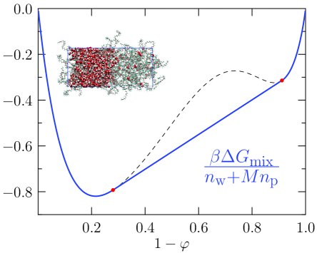
Figure 3: Mixing free energy and double tangent construction. INSET: Coexisting phases with chain-molecule volume fraction $1-\varphi\approx 0.34,0.99$. This coexistence is stable on the simulation time scale of 20 ns.

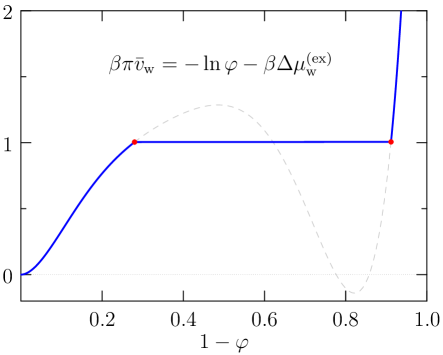
Figure 4: Osmotic pressures, Eq. (2.5). The coexistence points identified in FIG. 3 have equal osmotic pressures, as they should. The osmotic second virial coefficient is positive.

The $\chi_{\mathrm{WP}}\left(\varphi\right)$ (FIG. 3) describes separation of a water-poor solution from a water-rich phase. The osmotic pressure (FIG. 4) further characterizes the transition. To confirm the predicted phase separation, we simulated coexistence of water-rich and water-poor solutions (FIG. 3). The two fluids did indeed coexist stably on the simulation time scale of 20 ns, though the dynamics of the water-poor solution are distinctly sluggish: the self-diffusion coefficient of the water in the water-poor phase is about a 1/4th of that in the water-rich phase.

In assessing the coexisting water-poor phase, we note that these chains are short and the capping groups play a significant role. Comparable molecular-weight PEO chains with one hydroxyl and one methoxy termination are pastes at low water content. Methyoxy terminated PEO chains as small as two-times larger than the present case form crystals with Li electrolytes at these temperatures.Gadjourova et al. (2001) The difference between the predicted coexistence points and the compositions exhibited in FIG. 3 might be due to the assumption of ideal volumes of mixing. Though the excess volumes are small, they are largest in the interesting intermediate concentration $1-\varphi\approx 0.3$ region. This should receive further study.

IV Conclusions

The observations here should help in formulating a defensible molecular theory of PEO (aq) phase transitions. The interesting $\chi_{\mathrm{wp}}\left(\varphi\right)$ concentration dependence derives from long-ranged interactions.

This analysis provides straightforward predictions of osmotic pressures, not requiring detailed analysis of 2-body (or successive few-body) contributions. This realization should help in studies of osmotic stress.Cohen et al. (2009)

V Acknowledgement

The financial support of the Gulf of Mexico Research Initiative (Consortium for Ocean Leadership Grant SA 12-05/GoMRI-002) is gratefully acknowledged. We thank S. J. Paddison for helpful conversations.

VI Methods

Parallel tempering simulations, implementedChaudhari (2014) within GROMACS 4.5.3,van der Spoel et al. (2005) were used to enhance the sampling at the $T$ = 300 K temperature of interest. Parallel tempering swaps were attempted at a rate of 100/ns, which resulted in a success rates of 15-30%. The chain molecules were represented by the OPLS-aa force field,Jorgensen et al. (1996) and the SPC/E model was used for water.Berendsen et al. (1987) Long-range electrostatic interactions were treated in standard periodic boundary conditions using the particle mesh Ewald method with a cutoff of 0.9 nm. The Nosé-Hoover thermostat maintained the constant temperature and chemical bonds involving hydrogen atoms were constrained by the LINCS algorithm. After energy minimization and density equilibration at 300.4 K and $p$ = 1 atm, 40 replicas spanning 256-450 K, each at the same volume, were simulated for 10 ns. The pure liquid molar volumes were $\bar{v}_{\mathrm{w}}$ = 0.0178 dm³/mole, $\bar{v}_{\mathrm{p}}$ = 0.490 dm³/mole, so $M$ = 27.6. Configurations of the $T$ = 300.4 K replica were sampled every 0.5 ps for subsequent analysis. The packing, outer-shell and chemical terms were calculated separately using the replica at 300.4 K. 30,000 uniformly spaced trial insertions were used to estimate the packing term. The generalized reaction field method,Tironi et al. (1995) cutoff at 1 nm, was used to calculate the electrostatic contribution to the binding energies.

References

- Flory (1953) Flory, P. J. Principles of Polymer Chemistry; Cornell University Press: Ithaca, 1953.
- Huggins (1941) Huggins, M. L. J. Chem. Phys. 1941, 9, 440.
- Sharp et al. (1991) Sharp, K. A.; Nicholls, A.; Fine, R. F.; Honig, B. Science 1991, 252, 106–109.
- De Young and Dill (1990) De Young, L. R.; Dill, K. A. J. Phys. Chem 1990, 94, 801–809.
- Stillinger (1983) Stillinger, F. H. J. Chem. Phys. 1983, 78, 4654–4661.
- Parsegian and Zemb (2011) Parsegian, V.; Zemb, T. Curr. Op. Coll. & Interface Sci. 2011, 16, 618–624.
- Hill (1960) Hill, T. L. An Introduction to Statistical Thermodynamics; Addison-Wesley Publishing: Reading MA, 1960.
- Beck et al. (2006) Beck, T. E.; Paulaitis, M. E.; Pratt, L. R. Potential distribution theorum and statistical thermodynamics of molecular solutions; Cambridge University Press: New York, 2006.
- Doi (1995) Doi, M. Introduction to Polymer Physics; Oxford University, 1995.
- Bae et al. (1993) Bae, Y. C.; Shim, D. S., J. J .and Soane; Prausnitz, J. M. J. Appl. Poly. Sci. 1993, 47, 1193–1206.
- Chandler et al. (1983) Chandler, D.; Weeks, J. D.; Andersen, H. C. Science 1983, 220, 787–794.
- Shah et al. (2007) Shah, J. K.; Asthagiri, D.; Pratt, L. R.; Paulaitis, M. E. J. Chem. Phys. 2007, 127, 144508 (1–7).
- Pohorille and Pratt (2012) Pohorille, A.; Pratt, L. R. Orig. Life Evol. Biosp. 2012, 42, 405–409.
- Eliassi and Modarress (1999) Eliassi, A.; Modarress, H. J. Chem. & Eng. Data 1999, 44, 52–55.
- Zafarani-Moattar and Tohidifar (2006) Zafarani-Moattar, M. T.; Tohidifar, N. J. Chem. & Eng. Data 2006, 51, 1769–1774.
- Zafarani-Moattar and Tohidifar (2008) Zafarani-Moattar, M. T.; Tohidifar, N. J. Chem. & Eng. Data 2008, 53, 785–793.
- Kirkwood and Oppenheim (1961) Kirkwood, J. G.; Oppenheim, I. Chemical Thermodynamics; McGraw-Hill: New York, 1961.
- Paliwal et al. (2006) Paliwal, A.; Asthagiri, D.; Pratt, L. R.; Ashbaugh, H. S.; Paulaitis, M. E. J. Chem. Phys. 2006, 124, 224502.
- Chempath et al. (2009) Chempath, S.; Pratt, L. R.; Paulaitis, M. E. J. Chem. Phys. 2009, 130, 054113(1–5).
- Chaudhari et al. (2010) Chaudhari, M. I.; Pratt, L. R.; Paulaitis, M. E. J. Chem. Phys. 2010, 133, 231102.
- Chaudhari (2014) Chaudhari, M. I. Molecular simulations to study thermodynamics of polyethylene oxide solutions. Ph.D. thesis, Tulane University, 2014.
- Gadjourova et al. (2001) Gadjourova, Z.; Andreev, Y. G.; Tunstall, D. P.; Bruce, P. G. Nature 2001, 412, 520–523.
- Cohen et al. (2009) Cohen, J. A.; Podgornik, R.; Hansen, P. L.; Parsegian, V. A. J. Phys. Chem. B 2009, 113, 3709–3714.
- van der Spoel et al. (2005) van der Spoel, D.; Lindahl, E.; Hess, B.; Groenhof, G.; Mark, A. E.; Berendsen, H. J. C. J. Comp. Chem. 2005, 26, 1701–1718.
- Jorgensen et al. (1996) Jorgensen, W. L.; Maxwell, D. S.; Tirado-Rives, J. J. Am. Chem. Soc. 1996, 118, 11225–11236.
- Berendsen et al. (1987) Berendsen, H. J. C.; Grigera, J. R.; Straatsma, T. P. J. Phys. Chem. 1987, 91, 6269–6271.
- Tironi et al. (1995) Tironi, I. G.; Sperb, R.; Smith, P. E.; van Gunsteren, W. F. J. Chem. Phys. 1995, 102, 5451.