redMaPPer IV: Photometric Membership Identification of Cluster Galaxies with 1% Precision

Abstract

In order to study the galaxy population of galaxy clusters with photometric data one must be able to accurately discriminate between cluster members and non-members. The redMaPPer cluster finding algorithm treats this problem probabilistically. Here, we utilize SDSS and GAMA spectroscopic membership rates to validate the redMaPPer membership probability estimates for clusters with $z\in[0.1,0.3]$. We find small — but correctable — biases, sourced by three different systematics. The first two were expected a priori, namely blue cluster galaxies and correlated structure along the line of sight. The third systematic is new: the redMaPPer template fitting exhibits a non-trivial dependence on photometric noise, which biases the original redMaPPer probabilities when utilizing noisy data. After correcting for these effects, we find exquisite agreement ($\approx 1\%$) between the photometric probability estimates and the spectroscopic membership rates, demonstrating that we can robustly recover cluster membership estimates from photometric data alone. As a byproduct of our analysis we find that on average unavoidable projection effects from correlated structure contribute $\approx 6\%$ of the richness of a redMaPPer galaxy cluster. This work also marks the second public release of the SDSS redMaPPer cluster catalog.

1 Introduction

Galaxy clusters are not only powerful cosmological probes (Henry et al., 2009; Vikhlinin et al., 2009; Mantz et al., 2010; Rozo et al., 2010; Clerc et al., 2012; Benson et al., 2013; Hasselfield et al., 2013; Planck Collaboration XX, 2013), they are also useful as galaxy evolution laboratories. Of particular interest are the relation between the mass of a cluster and the stellar mass and/or luminosity of its central galaxy (e.g. Sheldon et al., 2004; Lin & Mohr, 2004; Whiley et al., 2008; More et al., 2009, 2011; Pipino et al., 2011; Skibba et al., 2011; Edwards & Patton, 2012; Kravtsov et al., 2014), the satellite population (Skibba et al., 2007; Yang et al., 2009b; Wetzel & White, 2010; Budzynski et al., 2012; Nierenberg et al., 2012; Ruiz et al., 2013), or both (Lin et al., 2004; Mandelbaum et al., 2006; Hansen et al., 2009; Yang et al., 2009a; Watson & Conroy, 2013; Budzynski et al., 2014). Indeed, these relations are key predictions of semi-analytic models of galaxy formation (Liu et al., 2010; Quilis & Trujillo, 2012), of hydrodynamic simulations that aim to resolve galaxy formation (Kravtsov et al., 2005; Weinberg et al., 2008; Feldmann et al., 2010; McCarthy et al., 2010, 2011; Martizzi et al., 2012; Le Brun et al., 2013; Ragone-Figueroa et al., 2013; Planelles et al., 2013), and of the popular sub-halo abundance matching scheme (Conroy et al., 2006; Guo et al., 2010; Behroozi et al., 2010; Reddick et al., 2013; Kravtsov, 2013; Hearin et al., 2013). Similarly, a comparison of the baryon budget in galaxy clusters to the cosmic mean can provide valuable clues about the role of feedback and galaxy formation on the star formation efficiency as a function of halo mass (Gonzalez et al., 2007; Giodini et al., 2009; Andreon, 2010; Laganá et al., 2011; Neistein et al., 2011; Leauthaud et al., 2012; Lin et al., 2012; Gonzalez et al., 2013). Irrespective of the specific question being asked, any observational study that addresses these questions must be able to robustly discriminate between galaxy cluster members and unassociated galaxies along the line of sight.

Here, we investigate the ability of the redMaPPer cluster finding algorithm (Rykoff et al., 2014, hereafter Paper I) — a new photometric algorithm specifically optimized for multi-band photometric surveys like the Sloan Digital Sky Survey (SDSS), the Dark Energy Survey (DES), and the Large Synoptic Survey Telescope (LSST) — to distinguish between cluster and non-cluster galaxies. Specifically, redMaPPer assigns a red membership probability $p_{\mathrm{RM}}$ to every galaxy in a cluster field. This probability is photometrically estimated, and includes some assumptions that are known to be incorrect: redMaPPer ignores both the existence of blue cluster galaxies and of correlated structure along the line of sight. The goal of this paper is to investigate the impact these systematics have on the redMaPPer red membership probabilities.

In order to test the redMaPPer probabilities we rely on spectroscopic data from the SDSS (SDSS DR10, Ahn et al., 2013) and from the Galaxy and Mass Assembly survey (GAMA, Driver et al., 2009). Specifically, given a bin of spectroscopic galaxies with fixed photometric membership probability $p_{\mathrm{RM}}$, we empirically determine the fraction of red galaxies that are spectroscopic cluster members, and compare this fraction to $p_{\mathrm{RM}}$. As a by product of this analysis, we are also able to place a tight constraint on the impact of projections from correlated structure on redMaPPer cluster richness. We emphasize that spectroscopic membership rates may not be trivially related to halo membership rates, and that this relation must necessarily depend on the halo definition being adopted (e.g. Biviano et al., 2006; Cohn et al., 2007; Serra & Diaferio, 2013). Our work is exclusively concerned with the “translation” between photometric to spectroscopic membership rates.

The layout of the papers is as follows: section 2 describes the data sets we use. Section 3 describes how we estimate the spectroscopic membership rates for red galaxies. Section 4 presents the result of our spectroscopic membership rates before and after accounting for the biases in the redMaPPer membership probability estimates, which are also detailed in this section. Section 5 summarizes our results and presents a brief discussion. Appendix A describes in detail our characterization of the photometric noise bias in the redMaPPer $\chi^{2}$ estimates.

We note that this work relies on the redMaPPer v5.10 cluster catalog, an updated version of the redMaPPer v5.2 cluster catalog presented in in Paper I. Appendix B summarizes the changes and updates to the redMaPPer catalog relative to Paper I. With this work we make the new redMaPPer cluster catalog publicly available at http://risa.stanford.edu/redmapper.

2 Data

2.1 redMaPPer

redMaPPer is a red-sequence photometric cluster finding algorithm that has been applied to SDSS DR8 photometric data (Aihara et al., 2011). This galaxy catalog contains $\approx 14,000\ \deg^{2}$ of imaging, which we reduce to $\approx 10,000\ \deg^{2}$ of contiguous high quality observations using the mask from the Baryon Acoustic Oscillation Survey (BOSS) (Dawson et al., 2013). redMaPPer uses the 5-band ($ugriz$) data available for every galaxy, and imposes a limiting magnitude of $i<21.0$. For further details on the various cuts and data handling employed by redMaPPer, we refer the reader to Paper I. As mentioned above, the catalog employed in this work is an updated version from that presented in Paper I, with the relevant updates summarized in Appendix B.

Additionally, we have run the redMaPPer algorithm on SDSS Stripe 82 (S82) coadd data (Annis et al., 2011). This catalog consists of $275\,\mathrm{deg}^{2}$ of $ugriz$ coadded imaging over the equatorial stripe that is roughly 2 magnitudes deeper than the single-pass SDSS data used for the DR8 catalog. Due to the higher redshift cutoff of the redMaPPer catalog in S82 data (we are roughly volume limited to $z<0.7$), most of our member galaxies are $u$-band dropouts. This, combined with the challenges of accurate calibration of the $u$-band data, led us to only use the $griz$ catalogs for input into redMaPPer. We note that this catalog was used exclusively for demonstrating the existence of photometric noise bias in our membership probability estimates, as discussed in detail in Appendix A. The stripe 82 catalog is not being made public at this time.

To create the input galaxy catalog for redMaPPer, we use similar flag cuts as those used for DR8, described in Paper I. In addition, we clean all galaxies that have magnitude errors that are gross outliers for typical galaxies at their observed magnitude. As in Paper I, total magnitudes are determined from $i$-band CMODEL_MAG and colors from $griz$ MODEL_MAG. To account for differences in photometric calibration and survey depth, the redMaPPer red-sequence calibration is performed in the S82 data as usual, irrespective of the DR8 data.

For reference, we briefly summarize the most salient features of the redMaPPer algorithm. redMaPPer is a matched filter algorithm. The most important filter characterizes the color of red-sequence galaxies as a function of redshift, which is self-calibrated by relying on clusters with spectroscopic redshifts. Having calibrated the filters describing the red-sequence of galaxy clusters as a function of redshift (amplitude, slope, and scatter), we use this information to tag each galaxy in the vicinity of a galaxy cluster with the probability $p_{\mathrm{RM}}$ of being a red cluster galaxy. The richness $\lambda$ is defined as the sum of the membership probabilities over all galaxies,

$$\lambda=\sum p_{\mathrm{RM}}.$$ (1)

Here, unless otherwise specified, we will restrict our analysis of the DR8 redMaPPer clusters to systems in the redshift range $z\in[0.1,0.3]$ with at least 20 galaxy counts. This results in $\approx 7000$ galaxy clusters spread over $\approx 10^{4}\ \deg^{2}$. The lower redshift limit reflects the lowest redshift at which redMaPPer is expected to be properly calibrated, while the high redshift cutoff ensures that the redMaPPer catalog is volume limited over the redshift range analyzed. The corresponding S82 redMaPPer catalog contains nearly 2000 clusters above our selection threshold of 20 galaxy counts, and the catalog is volume limited over the redshift range $z\in[0.1,0.7]$.

2.2 Spectroscopic Data

Our spectroscopic membership test relies on two distinct spectroscopic data sets. The first is SDSS DR10 (Ahn et al., 2013). DR10 combines all available spectroscopy from the SDSS through DR9 and new spectra acquired as part of the BOSS experiment. The total number of galaxy spectra in DR10 is 927,844, comprising a magnitude-limited sample (main sample Strauss et al., 2002), the SDSS Luminous Red Galaxy sample (LRG Eisenstein et al., 2001), and the BOSS targets, which includes an approximately constant stellar mass sample at high redshifts (CMASS) and a low redshift red galaxy sample (Dawson et al., 2013).

The second spectroscopic data set used is from the Galaxy And Mass Assembly survey (GAMA). GAMA is a magnitude-limited ($r<19.8$) spectroscopic survey of $\approx 300,000$ galaxies over $\approx 290\ \deg^{2}$, carried out using the AAOmega multi-object spectrograph on the Anglo-Australian Telescope (Driver et al., 2009). Here, we utilize GAMA data through the second data release and apply a quality flag $\geq 3$ cut, which includes $\approx 70,000$ galaxy redshifts over $\approx 48\ \deg^{2}$, all of which overlaps with the footprint of the redMaPPer cluster catalog.

In order to assign spectra from either SDSS or GAMA to the redMaPPer photometric member list of galaxies we rely on positional matching using a 1” angular aperture. To test the validity of this procedure as well as the robustness of the SDSS and GAMA redshifts, we perform this angular matching between the SDSS DR 10 and GAMA spectroscopic catalogs, and then study the distribution of the redshift difference $\Delta z=|z_{\mathrm{SDSS}}-z_{\mathrm{GAMA}}|$.

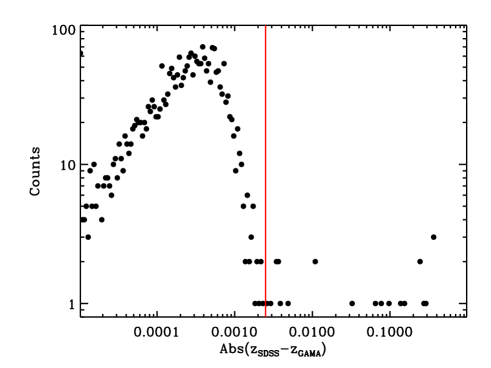
Figure 1: Number of galaxies within logarithmically spaced bins of $\Delta z=|z_{\mathrm{SDSS}}-z_{\mathrm{GAMA}}|$. Redshifts offsets to the right of the red vertical line are considered catastrophic failures, and represent $0.9\%$ of the objects.

Figure 1 shows the distribution of $\Delta z$ in logarithmically spaced bins. We see that there is a tail of discrepant redshifts starting at $\Delta z\approx 0.0025$, marked by the vertical red line. The total fraction of objects with a redshift difference larger than this is $0.9\%$, which we adopt as our estimate of the spectroscopic redshift failure rate, which contributes to our systematic uncertainty for the spectroscopic membership rate of photometric cluster members.

3 Selecting Red Spectroscopic Cluster Members

We wish to test the redMaPPer membership probabilities by comparing to spectroscopic membership rates. That is, if we select redMaPPer galaxies with membership probability $90\%$, and the redMaPPer membership probabilities are correct, then 90% of the selected galaxies ought to be spectroscopic cluster members. The first step in performing this test then is to describe how we estimate the spectroscopic membership rate of a set of galaxies.

3.1 Red Galaxy Spectroscopic Membership Rates

Given a galaxy cluster with velocity dispersion $\sigma_{v}$, we define a spectroscopic member to be a galaxy within a projected aperture $R_{\lambda}$ (see below) of a cluster, and whose velocity along the line of sight satisfies

$$|v|\leq N_{\mathrm{mem}}\sigma_{v}$$ (2)

where $N_{\mathrm{mem}}$ is a fiducial threshold, and $\sigma_{v}(\lambda,z)$ is the velocity dispersion of a cluster of richness $\lambda$ at redshift $z$. The radius $R_{\lambda}$ is the radius used by redMaPPer to estimate the cluster richness, and is related to the cluster richness via

$$R_{\lambda}=1.0\ h^{-1}\mbox{Mpc}\left(\frac{\lambda}{100}\right)^{0.2}.$$ (3)

One obvious problem with defining cluster membership via equation 2 is that cluster membership depends on the adopted membership cut $N_{\mathrm{mem}}$. We can account for this difficulty by assuming that the line of sight velocity distribution of galaxies is Gaussian. Specifically, if $N_{obs}(N_{\mathrm{mem}})$ is the number of spectroscopic galaxies obtained using a velocity cut $|v|\leq N_{\mathrm{mem}}\sigma_{v}$, the completeness-corrected number of members is

$$N_{\mathrm{tot}}=N_{obs}/\mathrm{erf}(N_{\mathrm{mem}}/\sqrt{2}).$$ (4)

If the velocity distribution were exactly Gaussian, the above definition would result in spectroscopic membership estimates that are independent of the adopted $N_{\mathrm{mem}}$ cut. In practice, we find that our spectroscopic membership rates are robust to changes in $N_{\mathrm{mem}}$ over the range $N_{\mathrm{mem}}\in[1,2.5]$ at the $1\%$ level, which we adopt as the associated systematic uncertainty. We choose $N_{\mathrm{mem}}=2.0$ as our fiducial membership threshold. We add in quadrature the systematic uncertainty in the spectroscopic membership rate due to our choice of $N_{\mathrm{mem}}$ to the spectroscopic redshift failure rate to arrive at a net systematic uncertainty of $1.3\%$. For reference, at the pivot point of our data, a $2\sigma_{v}$ cut in redshift corresponds to a $\approx 10\ h^{-1}\mbox{Mpc}$ separation along the line-of-sight.

Now, as was noted in the introduction, the redMaPPer probability $p_{\mathrm{RM}}$ is meant to describe the probability that a galaxy is a red cluster galaxy. Since blue cluster galaxies exist, we do not expect the redMaPPer membership probability $p_{\mathrm{RM}}$ to agree with the total fraction of spectroscopic cluster members, as some of those members will not be red galaxies. We must therefore limit ourselves to red galaxies when computing the spectroscopic membership rate.

This is easily done: let $p_{\mathrm{red}}$ be the probability of a galaxy being a red galaxy. Given $N$ galaxies each with a red probability $p_{\mathrm{red}}$, the total number of red galaxies is simply the sum total of the red membership probabilities. To obtain the total number of red cluster members, one simply restricts the sum to galaxies with $|v|\leq N_{\mathrm{mem}}\sigma_{v}$, exactly as before. If the total number of galaxies is $N$, the completeness-corrected red spectroscopic membership rate is simply

$$r_{\mathrm{spec}}=\frac{1}{\mathrm{erf}(N_{\mathrm{mem}}/\sqrt{2})}\frac{1}{N}\sum_{|v|\leq N_{\mathrm{mem}}\sigma_{v}}p_{\mathrm{red}}.$$ (5)

Equation 5 is the fundamental equation we use to determine the spectroscopic membership rate that is to be compared to the redMaPPer membership probabilities. In the following two sections, we describe how we estimate $\sigma_{v}$ and $p_{\mathrm{red}}$ for every cluster and galaxy respectively.

3.2 Estimating Velocity Dispersions

In the previous section we described how to estimate the cluster membership rate for galaxies in clusters of known velocity dispersion. Unfortunately, our spectroscopic data set is such that the typical number of galaxy spectra per cluster is low, so it is impossible for us to provide robust estimates of the velocity dispersion of individual clusters. Instead, we first calibrate the scaling relation between cluster velocity dispersion and cluster richness, and then use the velocity dispersions estimated from this scaling relation to determine cluster membership.

We calibrate the $\sigma_{v}$–$\lambda$ scaling relation as follows. First, we select all redMaPPer clusters whose central galaxy has a spectroscopic redshift, and then search for spectroscopic galaxies within the cluster radius $R_{\lambda}$ of each such cluster, irrespective of whether or not the galaxies are included in the cluster member list. In order to maximize our statistics, we employ both SDSS DR10 and GAMA spectroscopy. For each central–satellite par, we compute the velocity offset

$$v=c\frac{z_{\mathrm{sat}}-z_{\mathrm{cen}}}{1+z_{\mathrm{cen}}}$$ (6)

where $c$ is the speed of light.

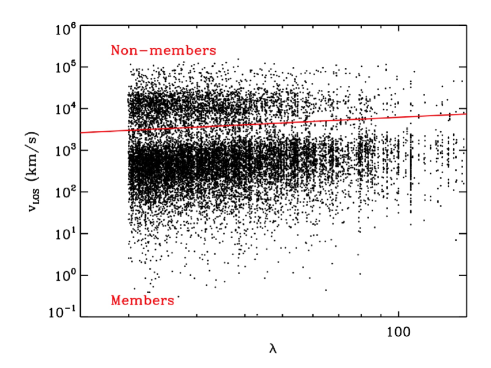
Figure 2: Line-of-sight velocities of spectroscopic central–satellite pairs of redMaPPer galaxy clusters. The red line shows the initial split into spectroscopic members and non-cluster members used to initialize the calibration of the velocity dispersion of the clusters.

Figure 2 shows the velocity offset $v$ of each central–satellite pair in the sample. There are two obvious populations: a sample with low velocity offsets ($|v|\lesssim 2000\ \mathrm{km/s})$, and a population of high velocity offsets. We perform an initial selection criteria for spectroscopic members via

$$|v|\leq(3000\ \mathrm{km/s})(\lambda/20)^{0.45}$$ (7)

shown in Figure 2 as a red line.

We model the velocity distribution of cluster satellite galaxies as a Gaussian of mean $\left\langle v\right\rangle=0$ with and a velocity dispersion $\sigma_{v}$ that is richness and redshift dependent,

$$\sigma_{v}(\lambda,z_{\mathrm{cen}})=\sigma_{p}\left(\frac{1+z_{\mathrm{cen}}}{1+z_{p}}\right)^{\beta}\left(\frac{\lambda}{\lambda_{p}}\right)^{\alpha}.$$ (8)

In the above expression, $\lambda_{p}$ is a pivot point chosen a priori to be the median richness of the cluster sample ($\lambda_{p}=33.336$), and $z_{p}$ is the median cluster redshift of all velocity pairs ($z_{p}=0.171$). $\sigma_{p}$ is the velocity dispersion of a cluster of richness $\lambda_{p}$ at the pivot redshift, and $\alpha$ and $\beta$ characterize the dependence of the velocity dispersion with cluster richness and redshift respectively.

We model the contribution of non-cluster members as a uniform background of spectroscopic galaxies. The full likelihood for any one galaxy is

$$\mbox{$\cal{L}$}_{i}=pG(v_{i})+(1-p)\frac{1}{2v_{\mathrm{max}}}$$ (9)

where $v_{\mathrm{max}}$ is the maximum velocity cut used to define the sample of candidate members. Here, $G(v_{i})$ is a Gaussian of mean zero and velocity dispersion $\sigma_{v}(\lambda,z_{\mathrm{cen}})$. The model parameters are $p$, $\sigma_{p}$, $\alpha$, and $\beta$, and the total likelihood is obtained by multiplying the individual likelihoods for every central–satellite pair,

$$\mbox{$\cal{L}$}=\prod_{i}\mbox{$\cal{L}$}_{i}.$$ (10)

Our best fit parameters are obtained by maximizing this likelihood.

To find our best fit parameters, we initialize our fits by setting $\alpha=0.45$ based on a “by eye” fit (e.g. Figure 2). We further set $\beta=0$ (i.e. ignore redshift evolution), and do a Gaussian fit to the velocity histogram obtained by stacking all clusters, irrespective of richness. The resulting width is adopted as the initial value for the amplitude $\sigma_{p}$. We then refit the data using our likelihood method after applying a selection cut

$$|v|\leq N_{\mathrm{cut}}\sigma_{v}$$ (11)

with $N_{\mathrm{cut}}=5.0$, so that the constant background is most representative of the areas immediately adjacent to the cluster member population. We refit, and the procedure is iterated until convergence. We arrive at

$$\lambda_{p} = 33.336$$ (12)

$$z_{p} = 0.171$$ (13)

$$\sigma_{p} = (618.1\pm 6.0)\ \mathrm{km/s}$$ (14)

$$\alpha = 0.435\pm 0.020$$ (15)

$$\beta = 0.54\pm 0.19$$ (16)

$$p = 0.9163\pm 0.0042$$ (17)

All errors are estimated using $10^{3}$ bootstrap resamplings of the velocity pairs, and are nearly uncorrelated.

We have further repeated the above procedure setting $N_{\mathrm{cut}}=6.0$. The difference in the recovered parameters is completely insignificant, except for the background amplitude parameter $p$ which must, of course, vary. We note that this robustness was only achieved when modeling the background. In particular, utilizing $N_{\mathrm{cut}}\in[2,3]$ with no background modeling results in systematic errors at the $\sim 8\%$ level, with the results being clearly dependent on $N_{\mathrm{cut}}$.

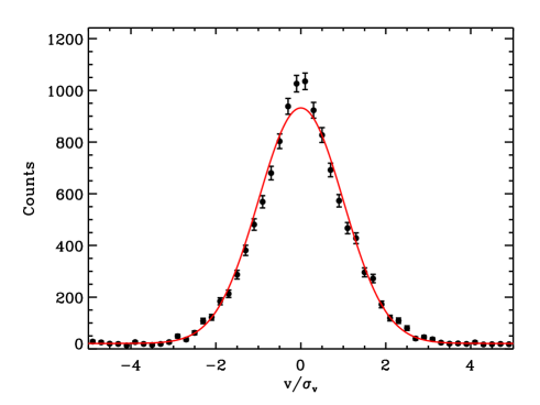
Figure 3: Distribution of the line-of-sight velocity $v$, normalized by the expected velocity dispersion $\sigma_{v}$ of the cluster, for all central–satellite pairs in our sample. The red curve is our best fit model (i.e. a gaussian of zero mean and width unity, and a flat background of non cluster galaxies). The amplitude is set by demanding that the total number of galaxy counts in the model curve exactly match the total number of counts in the data.

Figure 3 compares the distribution of normalized line-of-sight velocity offsets $v/\sigma_{v}$ for central–satellite pairs in our sample. The red line is a Gaussian of zero mean and unit variance, to which we have added the appropriate background model as per our best fit. The curve has been normalized so that the integral is equal to the total number of velocity pairs in the plot. Our model is not a good fit to the data ($\chi^{2}/dof=96.0/26$ for $v/\sigma_{v}\in[-3,3]$); the data is somewhat more sharply peaked than the unit Gaussian at $v\approx 0$. Consequently, it is not appropriate to use our likelihood to estimate the confidence interval of our best fit parameters, thereby explaining our reliance of bootstrap resampling. We emphasize, however, that the goal of this work is not to perform a detailed calibration of the $\sigma_{v}$–$\lambda$ relation: our main interest is to be able to identify cluster members from spectroscopic data, and our model suffices for this task. In particular, as noted earlier, the systematic error in our spectroscopic membership rates due to using a Gaussian model as per equation 4 is only 1%. A detailed analysis of the $\sigma_{v}$–$\lambda$ relation will be presented in a future paper.

Finally, we consider how uncertainty in our scaling relation impacts our spectroscopic membership rates. Varying the amplitude of the relation by its allotted error, we find that the recovered membership rates vary by $\pm 0.4\%$. Added in quadrature to the above error estimate we arrive at a total systematic error of $1.4\%$. Varying the remaining scaling relation parameters results in a negligible ($\leq 0.1\%$) change in the membership rates. This easily understood: changing the richness or redshift slopes will increase the membership rate on one side of the pivot point while simultaneously decreasing the membership rate on the opposite side of the pivot point. Because our pivot point is chosen to be at the median cluster richness/redshift, these two perturbations very nearly cancel each other.

3.3 When is a Galaxy Red?

We determine whether a galaxy is red or not by evaluating the goodness of fit of the redMaPPer red-sequence template. Roughly speaking, a galaxy is red if the red sequence template fit provides a good fit to its photometry (i.e. has a low $\chi^{2}$). In practice, however, our treatment of red galaxies is more sophisticated as detailed below.

The left panel of Figure 4 shows the distribution of $\chi^{2}$ — the goodness of fit of the redMaPPer red-sequence template to the galaxy photometry — for all GAMA galaxies with $z\in[0.1,0.3]$, as evaluated at each galaxy’s spectroscopic redshift (the red-sequence template is redshift dependent, see Paper I for details). Also shown is the $\chi^{2}$ distribution obtained using SDSS spectra only (dashed curve). In both cases, we have normalized the distributions to equal unity at their corresponding red peaks.

Also shown with a red curve is a $\chi^{2}$ distribution with 4 degrees of freedom (there are 4 colors), which we expect to be a good descriptor of the red wings of the $\chi^{2}$ distributions above. To fit the distribution of $\chi^{2}$ values with a $\chi^{2}$ distribution (allowing for an overall normalization factor only), it is imperative that the fit be performed over a $\chi^{2}$ range over which there is no contamination by non-red galaxies. Here, we have normalized the $\chi^{2}$ distribution by demanding that the integral of the $\chi^{2}$ distribution over the range $\chi^{2}\in[0,4]$ agree with that of the empirical distribution.

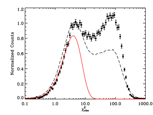
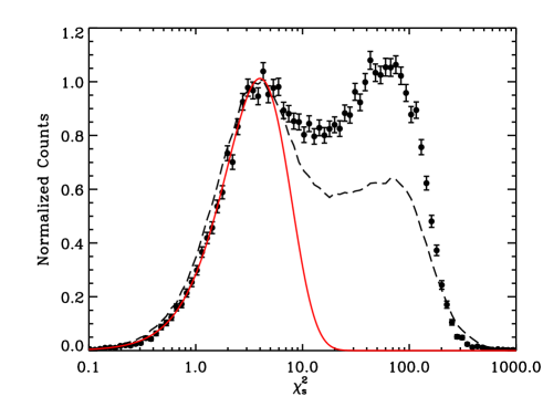
Figure 4: Left panel: Distribution of the goodness-of-fit statistic $\chi_{\mathrm{obs}}^{2}$ for all GAMA galaxies (points with error bars). $\chi_{\mathrm{obs}}^{2}$ is the goodness of fit of each galaxy’s photometry to the redMaPPer red-sequence template at the galaxy’s spectroscopic redshift. The GAMA data is normalized to unity at its left-peak value, estimated by fitting a cubic function to the data points around the peak. The dashed line is the corresponding distribution for all SDSS DR10 spectroscopic galaxies. Also shown for reference is a $\chi^{2}$ distribution with four degrees of freedom (red line), normalized so as to have the same integral as the GAMA data over the range $\chi_{\mathrm{obs}}^{2}\in[0,4]$. Right panel: As left panel, but using the rescaled $\chi^{2}$ values that correct for the effects of photometric noise bias.

If our covariance matrices were all exactly correct, the red wings of the SDSS and GAMA galaxies should fall directly on top of each other, and they would agree with the red curve. This is clearly not the case. As we show in Appendix A, our $\chi^{2}$ values suffer from photometric noise biases, and it is this bias which is responsible for the differences seen in the left panel of Figure 4.

In Appendix A we demonstrate the photometric noise bias in our $\chi^{2}$ values can be removed by rescaling our $\chi^{2}$ values via

$$\chi_{\mathrm{s}}^{2}=\exp(-s)\chi_{\mathrm{obs}}^{2}.$$ (18)

where $s$ accounts for the bias in our observed $\chi^{2}$. The bias $s$ is unique to each galaxy, and depends on each galaxy’s photometric errors. For details, see Appendix A.

The right panel in Figure 4 shows the distribution of the rescaled $\chi_{\mathrm{s}}^{2}$ values for SDSS and GAMA, as well as our reference $\chi^{2}$ distribution. As before, the $\chi^{2}$ distribution is normalized based on the integrated counts of the empirical distribution for $\chi^{2}\in[0,4]$. We see that the agreement between the various distributions has been dramatically improved. For the rest of this section, we rely exclusively on the rescaled $\chi_{\mathrm{s}}$ values for every galaxy whenever we refer to $\chi^{2}$. Nevertheless, we keep the subscript ‘s’ to make the rescaling explicit throughout.

The agreement between a $\chi^{2}$ distribution and the distribution of $\chi_{\mathrm{s}}^{2}$ values for spectroscopic galaxies seen in the right panel of Figure 4 enables us to define a probability $p_{\mathrm{red}}$ for any given galaxy to be a red galaxy. Specifically, let $\rho_{\mathrm{red}}$ and $\rho_{\mathrm{tot}}$ be the distribution of $\chi^{2}$ values for red galaxies and all galaxies respectively. The distribution $\rho_{\mathrm{red}}$ is defined to be a $\chi^{2}$ distribution with 4 degrees of freedom, but we demand that the integral of this distribution over the region $\chi^{2}\in[0,4]$ match the integral of the empirical distribution of $\chi_{\mathrm{s}}^{2}$ values over the same range. The probability that a galaxy of a given $\chi^{2}$ is a red galaxy is simply

$$p_{\mathrm{red}}=\frac{\rho_{\mathrm{red}}}{\rho_{\mathrm{tot}}}.$$ (19)

3.4 Environmental and Luminosity Dependences of the Red Fraction

The probability $p_{\mathrm{red}}$ depends of both environment and galaxy luminosity; after all, bright galaxies tend to be red, and cluster galaxies tend to be red. We investigate how the distribution of $\chi_{\mathrm{s}}^{2}$ values depends on both galaxy luminosity and environment by considering 4 different galaxy subsamples. The different samples are

• All GAMA galaxies with $z\in[0.1,0.3]$.

• All GAMA galaxies in $z\in[0.1,0.3]$ which are also spectroscopic cluster members ($2\sigma_{v}$ cut).

• All bright GAMA galaxies with $z\in[0.1,0.3]$.

• All dim GAMA galaxies with $z\in[0.1,0.3]$.

Note that we have restricted ourselves to GAMA spectroscopy (which has a magnitude-limited target selection) in order to avoid any biases due to color selection in SDSS targeting. To define bright and dim galaxies, we rank order the GAMA galaxies by $m-m_{*}(z)$, where $m_{*}(z)$ is the apparent luminosity of an $L_{*}$ galaxy utilized by the redMaPPer algorithm. The sample is then split into thirds, with the bright sample being the brightest third, and the dim sample being the dimmest third.

The left panel of Figure 5 shows the $\chi_{\mathrm{s}}^{2}$ distribution of each of our galaxy samples, as labelled. It is immediately apparent that irrespective of any selection effects, the red wing of the $\chi_{\mathrm{s}}^{2}$ distribution is well described by a $\chi^{2}$ distribution with 4 degrees of freedom. Additionally, there is an obvious luminosity and environmental dependence of the $\chi_{\mathrm{s}}^{2}$ distributions: dim galaxies have a much larger ratio of blue-to-red galaxies than bright galaxies, and cluster galaxies are very strongly preferentially red. Evidently, we must account for both the impact of environment and galaxy luminosity on the red fraction.

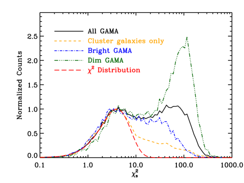
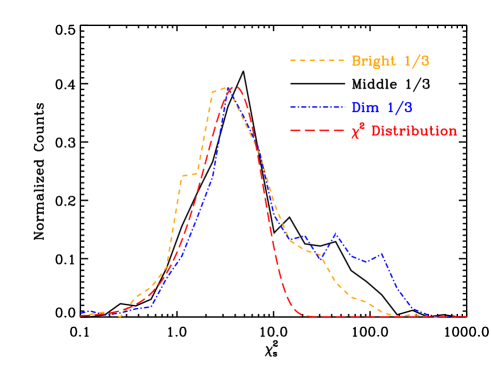
Figure 5: Left panel: Comparison of the $\chi_{\mathrm{s}}^{2}$ distribution of galaxies selected in a variety of ways, as labelled (see text for detailed descriptions). All distributions are normalized to unity at their left-most peak, and are well described by a $\chi^{2}$ distribution with 4 degrees of freedom (red dashed line). Right panel: Comparison of the $\chi_{\mathrm{s}}^{2}$ distribution of cluster galaxies for three different luminosity bins, as labelled. The red long-dash curve is a $\chi^{2}$ distribution with four degrees of freedom, normalized to have the same integral over the region $\chi^{2}\in[0,6]$ as the full data set. All empirical distributions are normalized to have the same integral over all space.

The right panel of Figure 5 shows the $\chi_{\mathrm{s}}^{2}$ distribution of cluster galaxies in three luminosity bins, each chosen to contain 1/3 of the available GAMA spectra. Due to the comparatively low number of spectra available for this analysis, we have decreased the redMaPPer richness threshold to $\lambda=10$ in order to make this plot. All histograms were normalized to an integral of unity, which makes evident the rather surprising result that the $\chi^{2}$ distribution of cluster galaxies is roughly luminosity independent.

In light of the above results, we combine all GAMA spectroscopic cluster galaxies into a single bin, and ignore any possible luminosity dependence of the $\chi^{2}$ distribution. We then fit the resulting distribution with a $\chi^{2}$ distribution with 4 degrees of freedom by demanding that the integral of the model agree with the data over the range $\chi^{2}\in[0,6]$, with $\chi^{2}\approx 6$ being roughly the largest $\chi^{2}$ value for which $p_{\mathrm{red}}=1$. This defines the distribution $\rho_{\mathrm{red}}$ which we use in equation 19 to estimate $p_{\mathrm{red}}$. Our resulting $p_{\mathrm{red}}(\chi_{\mathrm{s}}^{2})$ function is shown in Figure 6.

We fit the probability $p_{\mathrm{red}}(\chi_{\mathrm{s}})$ via

$$p_{\mathrm{red}}(\chi_{\mathrm{s}})=\frac{1}{2}\left[1-\mathrm{erf}\left(\frac{\ln(\chi_{\mathrm{s}}/\chi_{\mathrm{ref}})}{\sqrt{2}\sigma}\right)\right]$$ (20)

where $\chi_{\mathrm{ref}}$ and $\sigma$ are parameters to be fit for. We find

$$\ln\chi_{\mathrm{ref}} = 2.44\pm 0.08$$ (21)

$$\sigma = 0.28\pm 0.11$$ (22)

with the two parameters being nearly uncorrelated. Our best fit model for $p_{\mathrm{red}}(\chi_{\mathrm{s}})$ is also shown in Figure 6 as a solid black line. In all subsequent work, unless otherwise specified when we need to evaluate $p_{\mathrm{red}}(\chi_{\mathrm{s}})$, we will rely on our best fit model to do so. In particular, we use this best fit model to compute the red spectroscopic membership rates as per equation 5.

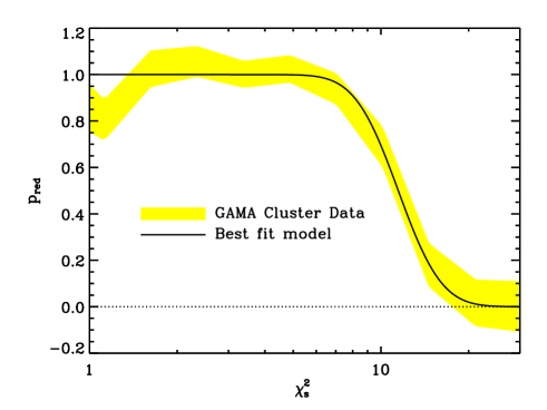
Figure 6: Probability $p_{\mathrm{red}}=\rho_{\mathrm{red}}/\rho_{\mathrm{tot}}$ (i.e. the red fraction) as a function of $\chi_{\mathrm{s}}^{2}$. The bands marks the empirical 68% confidence regions, while the black line shows our best fit model.

We note that the uncertainty associated with whether a galaxy is red or not implies a corresponding systematic uncertainty in the red spectroscopic membership rates. This uncertainty is easily dominated by the error in $\ln\chi_{\mathrm{ref}}$, which induces an error of $\pm 1.6\%$. When added in quadrature to our previous estimate of the systematic uncertainty, we arrive at a net systematic error of $2.1\%$ for our red spectroscopic membership rates.

4 The Spectroscopic Membership Test

4.1 Testing the redMaPPer Membership Probabilities

We compare the redMaPPer membership probabilities $p_{\mathrm{RM}}$ to the red spectroscopic membership rate as estimated via equation 5. Specifically, we collect redMaPPer cluster member galaxies into membership probability bins, and compute the mean membership probability of each bin. This mean probability is then compared to the measured spectroscopic membership rate.

The results of this comparison is shown in the left panel of Figure 8. The agreement between the photometric probabilities and the spectroscopic membership rates is reasonable, but there is an obvious bias: redMaPPer systematically overestimates the membership probabilities by $\approx 5\%$. As we now demonstrate, this bias is well understood and can be fully accounted for.

4.2 Understanding the Biases in the redMaPPer Probabilities

The bias in the redMaPPer probability estimates are a combination of three separate effects. Specifically,

1. Photometric noise bias in the redMaPPer $\chi^{2}$ values.

2. redMaPPer ignores correlated structure.

3. redMaPPer ignores blue cluster galaxies.

Consider first photometric noise biases in $\chi^{2}$. Our de-biased $\chi^{2}$ estimates are given by equation 42. Assuming these rescaled $\chi^{2}$ values are distributed via a $\chi^{2}$ distribution with four degrees of freedom, which we denote $\rho_{0}$, it follows that the distribution of the original $\chi^{2}$ values is

$$\rho=\exp(-s)\rho_{0}(\exp(-s)\chi_{\mathrm{obs}}^{2}).$$ (23)

The membership probability is therefore

$$p_{\mathrm{mem}} = \frac{\lambda\rho}{\lambda\rho+B}$$ (24)

$$= \frac{\lambda\rho_{0}(1+\epsilon_{\chi^{2}})}{(\lambda\rho_{0}+B)\left(1+(\lambda\rho_{0}\epsilon_{\chi^{2}})/(\lambda\rho_{0}+B)\right)}$$ (25)

$$= p_{\mathrm{RM}}\frac{1+\epsilon_{\chi^{2}}}{1+p_{\mathrm{RM}}\epsilon_{\chi^{2}}}$$ (26)

where $B$ is the background, $p_{\mathrm{RM}}$ is the original redMaPPer membership probability estimate, and

$$\epsilon_{\chi^{2}}=\frac{\rho(\chi_{\mathrm{obs}}^{2})}{\rho_{0}(\chi_{\mathrm{obs}}^{2})}-1.$$ (27)

Equation 26 allows us to correct the effects of photometric noise bias in $\chi^{2}$ on the redMaPPer probability $p_{\mathrm{RM}}$.

We can perform a similar calculation for the impact of correlated structure. Assuming that the correlated galaxy counts $N_{\mathrm{corr}}$ is a constant fraction $c$ of the cluster richness, we find

$$p_{\mathrm{mem}} = p_{\mathrm{RM}}\frac{1}{1+p_{\mathrm{RM}}c}$$ (28)

Finally, redMaPPer ignores the existence of blue galaxies. Consequently, the true probability that a galaxy is a red cluster member is not $p_{\mathrm{RM}}$, but rather $p_{\mathrm{mem}}$, where

$$p_{\mathrm{mem}} = \frac{N_{\mathrm{red}}}{N_{\mathrm{red}}+N_{\mathrm{blue}}+B}$$ (29)

$$= \frac{p_{\mathrm{RM}}}{1+p_{\mathrm{RM}}\epsilon_{\mathrm{blue}}}.$$ (30)

where

$$\epsilon_{\mathrm{blue}}=\frac{f_{\mathrm{blue}}(\chi^{2})}{1-f_{\mathrm{blue}}(\chi^{2})}$$ (31)

and $f_{\mathrm{blue}}(\chi^{2})=1-p_{\mathrm{red}}$ is the blue fraction as a function of $\chi^{2}$.

There is one additional effect that must be properly accounted for: as we vary the membership probability of galaxies, we must also vary the total cluster richness in concert, since the two are related by the constraint equation 1. A shift in cluster richness $\lambda=\lambda_{0}(1+\delta)$ will necessarily rescale all membership probabilities via

$$p_{\mathrm{mem}}=p_{\mathrm{RM}}\frac{1+\delta}{1+p_{\mathrm{RM}}\delta}$$ (32)

and vice versa. Given the probability rescaling detailed above, we re-estimate the cluster richness by summing up the new probabilities. This new richness estimate is used to compute the parameter $\delta$, which is then used to rescale the membership probabilities as per equation 32. The procedure is then iterated one more time. We find that additional iterations perturb our membership below the $0.5\%$ level, and are therefore negligible.

We note that while for pedagogical purposes we considered each perturbation in isolation, in practice we simultaneously consider the impact of all of the effects considered here. We find that the redMaPPer membership probabilities must be rescaled via

$$p_{\mathrm{mem}}=p_{\mathrm{RM}}\frac{1+\nu}{1+p_{\mathrm{RM}}(\mu+\nu+\mu\nu)}$$ (33)

where

$$\mu = \epsilon_{\mathrm{blue}}+c$$ (34)

$$\nu = \delta+\epsilon_{\chi^{2}}+\delta\epsilon_{\chi^{2}}.$$ (35)

4.3 Calibration of Projection Effects

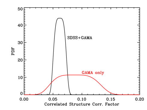
Figure 7: Posteriors on the mean fraction of red photometric cluster members selected by the redMaPPer algorithm that are not spectroscopic cluster members, but are instead contributed by correlated structures along the line of sight.

The parameter $c$ governing the impact of projection effects in redMaPPer clusters is unknown a priori. We utilize our spectroscopic membership test in order to calibrate the parameter $c$. Specifically, given a value of $c$, we can use equation 33 to rescale all of the membership probabilities for galaxies in the redMaPPer cluster member catalog, and compare these to the spectroscopic membership rates as per section 4.1. This allows us to compute a goodness-of-fit statistic $\chi_{\mathrm{test}}^{2}$, where we use the subscript “test” to distinguish this $\chi^{2}$ value from the other occurrences of $\chi^{2}$ in this manuscript. We have then

$$\chi_{\mathrm{test}}^{2}=\sum\frac{(f_{\mathrm{red}}^{(i)}-p_{\mathrm{mem}}^{(i)})^{2}}{\sigma_{i}^{2}}.$$ (36)

where the sum is over the membership probability bins. The error $\sigma_{i}$ is given by

$$\sigma_{i}=\frac{\sqrt{N_{\mathrm{specmems}}}}{N_{i}}$$ (37)

We adopte a likelihood $\mbox{$\cal{L}$}\propto\exp(-\chi_{\mathrm{test}}^{2})$, and grid in the parameter $c$ to measure the corresponding likelihood distribution, which we show in Figure 7. We fit for $c$ using both GAMA and SDSS+GAMA data sets, checking for consistency to guard ourselves against biases introduced by the impact of color selection in the SDSS spectroscopic targeting algorithm. We find consistent results between the two data sets. The 68% confidence interval for the SDSS+GAMA data set is $c=6.2\%\pm 0.8\%$ (see Figure 7). Finally, recall that the spectroscopic membership rates are themselves uncertain at the $\approx\pm 2.1\%$ level. Adding all of these quantities in quadrature we arrive at

$$c=6.2\%\pm 2.2\%.$$ (38)

This is an important observational constraint on any future model of projection effects. We again caution, however, that our spectroscopic membership rate is not equivalent to a halo membership rate, and in particular the relation between these two is necessarily dependent on the halo definition adopted, so the appropriate conversions must be undertaken when interpreting our results within the context of a halo model. The corresponding value for the parameter $\delta$ is $\delta=-0.094$. The dominant uncertainty in this analysis is the systematic error associated with our ability to determine whether a galaxy is red or not — i.e. the uncertainty in the probability $p_{\mathrm{red}}(\chi_{\mathrm{s}}^{2})$ — followed closely by the systematic error in the spectroscopic membership rate due to the non-Gaussian nature of the velocity distribution of galaxies in galaxy clusters.

4.4 Testing the Rescaled Membership Probabilities

Figure 8 compares the rescaled photometric membership probabilities $p_{\mathrm{mem}}$ to the red spectroscopic membership rates. We find the rescaled membership probabilities provide somewhat too good a fit to the spectroscopic data

$$\chi^{2}/dof=15.1/29.$$ (39)

The probability of finding a $\chi^{2}$ larger than observed is $\approx 98\%$ ($2.3\sigma$). It is likely that this low $\chi^{2}$ reflects a failure of our statistical modeling. For instance, at $p_{\mathrm{mem}}\approx 0.3$, there is a broad region where our rescaled probabilities appear to be biased somewhat low across many nominally independent points, suggesting that the points are not in fact statistically independent. Nevertheless, the agreement between the photometric and spectroscopic membership rates is remarkable.

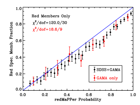
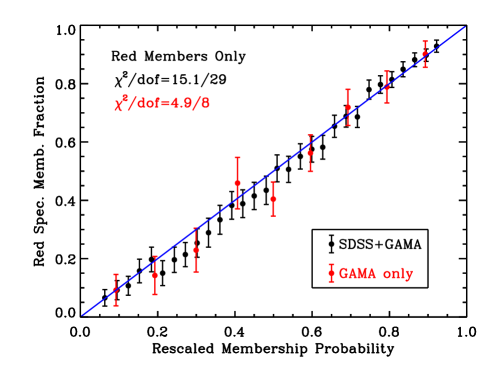
Figure 8: Left panel: Comparison of the redMaPPer membership probabilities to the red spectroscopic membership rate. The observed biases are due to the combination of three systematic effects: noise biases in the $\chi^{2}$ values used by redMaPPer, the fact that redMaPPer ignores the existence of both cluster galaxies and correlated structure. Right panel: As left panel, but after correcting for the three aforementioned systematic effects. The correction for projection effects introduces a free parameters that is being fit to the data, as reflected in the decrease in the degrees of freedom for the $\chi^{2}$ goodness-of-fit test.

5 Summary and Discussion

We have studied whether the photometrically estimated redMaPPer membership probabilities can be used to accurately determine whether any given galaxy is a red cluster member or not. The raw redMaPPer probabilities are biased relative to the observed spectroscopic membership rates, which is expected given that redMaPPer explicitly assumes that there are not blue galaxies in clusters, and that clusters have no correlated structure, both assumptions that are obviously incorrect a priori.

In addition, we have found that the redMaPPer $\chi^{2}$ values suffer from noise bias. This bias is typically $\approx 25\%$ for DR8 data, and could be thought of as a systematic bias in the estimate of the covariance matrix describing the red-sequence. Note that a $25\%$ bias in $\chi^{2}$ corresponds to a 12% bias in the red-sequence scatter, or $\approx 0.006$ mag. While it is not clear to us what the physical origin of this bias is, our work demonstrates that the noise bias can be empirically characterized and accounted for (see Appendix A).

Having identified the sources of bias in the membership probability estimates from redMaPPer, we corrected our probability estimates, including a fit for the amount of average contribution from correlated structure to the redMaPPer cluster richness. The corrected membership probabilities are observed to be in excellent agreement with the spectroscopic membership rate, with an overall systematic uncertainty of 2.4%. For reference, the systematic floor due to spectroscopic redshift failure rates is 0.9%. In other words, our calibration enables studies of the galaxy population of galaxy clusters from photometric data without incurring a significant degradation in the quality of the data relative to a fully spectroscopic data set.

Interestingly, as a byproduct of this analysis we were able to constrain the average contribution to a cluster’s richness due to projected structure in the low redshift Universe, finding that, on average, 6.2% of the richness of a galaxy cluster is due to non-cluster galaxies. This is an important observational constraint that can be used to better characterize the impact of projection effects on photometric cluster samples, for instance within the context of cluster cosmology in the DES or LSST. As noted in the text, we emphasize that interpreting our results within a halo model context requires calibration of how spectroscopic membership rates relate to halo membership, and that this relation clearly depends on the adopted halo definition.

Appendix A Photometric Noise Bias in $\chi^{2}$

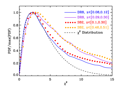
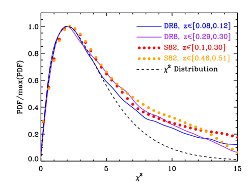
Figure 9: Left panel: Comparison of the $\chi^{2}$ distribution of all galaxies with a membership probability $p_{\mathrm{mem}}\geq 1\%$ for different data sets and different redshift bins, as labelled. S82 refers to redMaPPer clusters in stripe 82 data. Right panel: As left panel, but we have rescaled the $\chi^{2}$ values for the DR8 and S82 high redshift bins as per equation 18 by $s=0.25$.

It was mentioned in section 3.3 that we have discovered that the $\chi^{2}$ values obtained by redMaPPer suffer from photometric noise bias. The evidence for this bias is shown in Figure 9, where we show the $\chi^{2}$ distribution of all photometric galaxies with membership probability $p_{\mathrm{mem}}\geq 1\%$ in the vicinity of redMaPPer clusters (within a radius $R_{\lambda}$) for a variety of clusters in different redshift bins, as labelled. In the legend, DR8 refers to redMaPPer galaxy clusters in DR8, while S82 refers to redMaPPer galaxy clusters in Stripe 82.

It should be noted that the S82 redMaPPer catalog does not use $u$ band data, so the raw $\chi^{2}$ value from the S82 data is not directly comparable with that from DR8. We overplot the two by using density matching to relate the S82 $\chi^{2}$ values to the equivalent DR8 $\chi^{2}$ values. Given a galaxy with a $\chi^{2}$ value $\chi^{2}_{3}$ in stripe 82 (the subscript is the number of colors), the corresponding $\chi^{2}$ value in DR8 will be $\chi^{2}_{4}$, selected so as to match the cumulative distribution function of the respective $\chi^{2}$ distributions. That is, $\chi^{2}_{4}(\chi^{2}_{3})$ is defined via

$$\int_{0}^{\chi^{2}_{3}}dx\ \rho(x|3)=\int_{0}^{\chi^{2}_{4}}dx\ \rho(x|4).$$ (40)

This mapping allows us to rescale the $\chi^{2}$ value for every stripe 82 galaxy into its DR8 equivalent.

We see that the low z and high z DR8 clusters exhibit different $\chi^{2}$ distributions (blue line vs. purple line), which could in principle be due to galaxy/cluster evolution. We see, however, that the distribution of $\chi^{2}$ values for S82 clusters over the range $z\in[0.1,0.3]$ is identical to the z=0.1 DR8 distribution rather than the z=0.3 DR8 distribution. Evidently, the difference in the distribution of $\chi^{2}$ values between the low and high redshift DR8 samples is not intrinsic evolution, but rather increased photometric noise in the high redshift DR8 data. This is confirmed by selecting a stripe 82 redshift bin ($z\in[0.46,0.51]$) for which the median photometric noise of the cluster galaxies is equal to that of the $z=0.3$ DR8 galaxy sample. We see that these two distributions (orange points vs purple line) are identical.

We parameterize the noise bias in $\chi^{2}$ via a factor $s$ which rescales the observed $\chi^{2}$ to its correct value via equation 42. Evidently, the factor $s$ must be $s\approx 0$ for well measured galaxies, but $s>0$ for noisy galaxies. The question is: what does “noisy” mean? Since we are interested in red-sequence galaxies, the obvious answer is that the rescaling must become necessary when the observed width of the red-sequence becomes dominated by photometric errors rather than by its intrinsic width. Thus, if $\sigma_{\mathrm{obs}}$ is the photometric error in the galaxy color, and $\sigma_{\mathrm{int}}$ is the intrinsic width of the red-sequence in that galaxy color, we expect that the rescaling factor $s$ will take the form

$$s=s_{\mathrm{max}}\frac{\sigma_{\mathrm{obs}}^{2}}{\sigma_{\mathrm{obs}}^{2}+\sigma_{\mathrm{int}}^{2}}$$ (41)

where $s_{\mathrm{max}}$ is the maximum value of the rescaling parameter.

In practice, our photometric errors and red-sequence width are multi-dimensional, which requires a multi-dimensional generalization of equation 41. We make the ansatz

$$s=\frac{1}{4}s_{\mathrm{0}}\mathrm{Tr}\left(\mathbf{C}_{\mathrm{tot}}^{-1}\mathbf{C}_{\mathrm{obs}}\right)$$ (42)

where $\mathbf{C}_{\mathrm{tot}}$ is the total covariance matrix $\mathbf{C}_{\mathrm{tot}}=\mathbf{C}_{\mathrm{int}}+\mathbf{C}_{\mathrm{obs}}$, and $\mathbf{C}_{\mathrm{int}}$ is the covariance matrix describing the intrinsic scatter of the red-sequence. The $1/4$ prefactor accounts for the dimensionality of the covariance matrix. For diagonal matrices, we’d expect $s\leq s_{\mathrm{0}}$, with $s\rightarrow s_{\mathrm{0}}$ in the limit of very large photometric errors. In practice, we find that $s_{0}$ is roughly equal to the maximum value for $s$ observed in our galaxies, but it is not a strict upper bound. Note that since $\mathbf{C}_{\mathrm{int}}$ is a function of redshift, we expect $s_{\mathrm{0}}$ to have some mild redshift dependence.

To compute our best fit model for $s_{\mathrm{0}}$, we proceed as follows. First, we rescale our data as per equations 18 and 42. The cluster member galaxies are then binned to arrive at an empirical estimate of the rescaled $\chi^{2}$ distribution. This distribution is expected to match a $\chi^{2}$ distribution, so we construct a cost function $E(s_{\mathrm{0}})$ defined as the total square deviation between our empirical estimate and our model prediction (which is properly integrated over each $\chi^{2}$ bin). Our best fit model for $s_{\mathrm{0}}$ is that which minimizes our cost function. In order to ensure that the fit is done over a region that is well described by a $\chi^{2}$ distribution, we only fit the region $\chi^{2}_{s}\leq 4$. Further, we allow $s_{\mathrm{0}}$ to be redshift dependent, with $s_{\mathrm{0}}(z)$ being parameterized using spline interpolation. The model parameters are the values on the spline nodes, for which we set $z=0.08$, $z=0.28$, and $z=0.55$. We find that three nodes are sufficient to accurately model the full $z\in[0.08,0.55]$ redshift range.

The left panel in Figure 10 shows the distribution of rescaled $\chi^{2}$ values obtained using our best fit model for $s_{\mathrm{0}}(z)$. It is immediately apparent that our model does a good job of accounting for the bias introduced by photometric noise in our measurement. Importantly, the distribution of rescaled $\chi^{2}$ values is universal not only over the region $\chi^{2}\leq\chi^{2}_{\mathrm{cut}}$, but across the entire range of $\chi^{2}$ values that we probe.

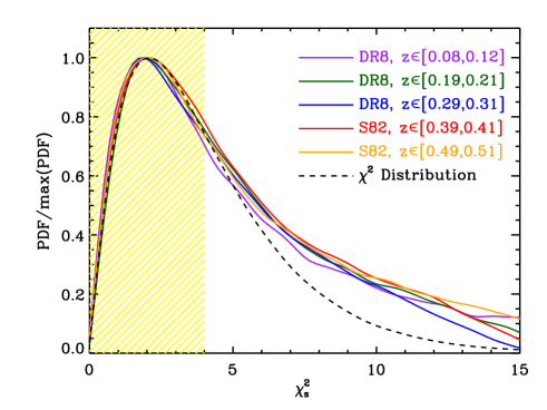
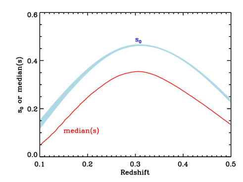
Figure 10: Left panel: Distribution of the rescaled $\chi^{2}$ values of cluster galaxies in DR8 as per equations 18 and 42 using our best fit model for $s_{\mathrm{0}}(z)$ for a variety of different redshifts, as labelled. The hatched yellow region denotes the range of $\chi^{2}$ values used in fitting for $s_{\mathrm{0}}$. Right panel: The 68% confidence band for $s_{\mathrm{0}}(z)$, as well as the median value of $s$ for all DR8 cluster galaxies as a function of redshift.

The right panel shows our best fit model for $s_{\mathrm{0}}(z)$, as well as the median shift $s(z)$ for cluster galaxies at redshift $z$. For $s_{\mathrm{0}}$, we show the 68% confidence band at each redshift, as determined by bootstrap resampling the cluster member galaxy catalog 100 times and then recomputing the best fit node values for each realization. In addition, we also show the median $s$ value of our cluster galaxies as a function of redshift.

Appendix B Updates to the redMaPPer Algorithm

The analysis in this paper relies on the redMaPPer catalog obtained using the redMaPPer code version 5.10, which includes a variety of updates and upgrades to version 5.2, used in Paper I. We summarize these changes here, and make the redMaPPer v5.10 catalog publicly available with this work.

In addition to fixing assorted minor bug fixes, the changes to the redMaPPer algorithm between v5.2 and v5.10 are:

1) Clusters are selected directly on the number of detected cluster galaxies. As with redMaPPer v5.2, our detection threshold is set to 20 detected cluster galaxies. In a region where no galaxies are masked (no star holes and where we are complete to the luminosity threshold), this is equivalent to a $\lambda>20$ threshold. However, if part of the cluster is masked, 20 galaxy detections must necessarily correspond to a richness threshold larger than 20. In redMaPPer v5.2, we set this threshold as a simple function of redshift, based on the average depth of the survey and ignoring the effects of star holes and boundaries. In v5.10, we directly set a threshold for each individual cluster to ensure 20 galaxies are detected. For fairly uniform surveys such as SDSS, this change has a very small impact on cluster selection. However, future surveys such as the Dark Energy Survey (DES) have much larger depth variations. In the interest of making our algorithm more generally applicable, we have applied this update when running on SDSS data as well.

2) All cuts used in defining richness are treated as smooth rather than sharp cuts. In redMaPPer v5.2, in the absence of masking the cluster richness was defined via

$$\lambda=\sum p_{i}$$ (43)

where $p_{i}$ is the membership probability of galaxy $i$. The sum was restricted to galaxies brighter than $0.2L_{*}$ and within a radial separation $R\leq R(\lambda)$, where $R(\lambda)$ is a richness-dependent aperture. Consequently, the above equation can be rewritten as

$$\lambda=\sum p_{i}\theta_{i}^{L}\theta_{i}^{R}$$ (44)

where the sum is now over all galaxies, and $\theta_{i}^{L}$ and $\theta_{i}^{R}$ are luminosity and radius dependent weights, which are top-hat functions for redMaPPer v5.2. It is clear from this that the richness definition is inherently unstable: there are always cases of galaxies that are just over or just under $0.2L_{*}$ in luminosity, and/or just inside or just outside the radius $R\leq R(\lambda)$. Therefore, small changes to either “edge” can result in macroscopic changes to the richness.

To overcome this difficulty, we now utilize soft cut-off weights. Specifically, we set

$$\theta_{i}^{L} = \frac{1}{2}\left[1+\mathrm{erf}\left(\frac{m_{\rm max}-m_{i}}{\sigma_{i}}\right)\right]$$ (45)

$$\theta_{i}^{R} = \frac{1}{2}\left[1+\mathrm{erf}\left(\frac{R(\lambda)-R}{\sigma_{R}}\right)\right],$$ (46)

where $m_{\rm max}$ is the magnitude corresponding to the $0.2L_{*}$ luminosity threshold or the survey limiting magnitude (whichever is brighter), $\sigma_{i}$ is the photometric error of galaxy $i$, and $\sigma_{R}=0.05\ h^{-1}\mbox{Mpc}$. This has a small impact on the richness of most galaxy clusters, while making the richness stable for those clusters with galaxies just inside or just outside our fiducial boundaries.

3) Cluster galaxy mask-fractions are now estimated taking into account the local survey depth. Galaxies are now selected based on the local depth of the SDSS imaging, which is estimated “on the fly” on a cluster by cluster basis. In Rykoff et al. (in prep), we describe a method for estimating the depth of a photometric survey based on the galaxy catalog. The idea is simple: given the effective sky noise, and assuming Poisson errors in the photon counts, one can derive a two-free parameter model that relates the magnitude of a source to its error. These two free parameters are the effective exposure time and the $10\sigma$ limiting magnitude of the image. We estimate the depth in each cluster field by selecting all galaxies within a $2.5\ h^{-1}\mbox{Mpc}$ aperture of the cluster center, and fitting our model to the resulting galaxy data. This information is utilized when computing mask-fraction corrections. Specifically, when computing mask fraction corrections, we generate Monte Carlo realizations of the cluster galaxies, and then perturb their magnitudes in accordance with the local depth to estimate the fraction of the cluster being masked.

4) Our propagation of the uncertainty introduced by masking into richness errors has been updated to make it significantly more stable. Specifically, in the presence of masking, the cluster richness is estimated via

$$\lambda(1-C)=\sum p_{i}$$ (47)

where $C$ is the fraction of the cluster being masked, which has an associated uncertainty $\sigma_{C}$. For details, see Paper I. We convert the uncertainty in $C$ into a richness error estimate via

$$\sigma_{\lambda}=\left|\frac{d\lambda}{dC}\right|\sigma_{C}.$$ (48)

In redMaPPer v5.2, the factor $d\lambda/dC$ was estimated numerically using a finite difference method. However, we found this procedure to be numerically noisy. Here, we rely on an alternative method for computing $d\lambda/dC$. Specifically, using the fact that the membership probability of a galaxy is $p=\lambda u/(\lambda u+b)$, and taking the differential of equation 47, we arrive at

$$dC=\sum\left(\frac{u}{\lambda u+b}\right)^{2}ud\lambda,$$ (49)

or simply

$$\frac{d\ln\lambda}{dC}=\frac{1}{\lambda}\frac{1}{\sum p^{2}}$$ (50)

where the sum is over the detected galaxies, and is evaluated using a fixed metric aperture. We plug this into equation 48 to get the error in the cluster richness given the fixed metric aperture. Note, however, that the aperture used for richness estimation itself depends on richness. Therefore, an increased richness leads to a larger aperture, which in turn leads to an even larger richness estimate. An increase in richness $d\ln\lambda_{0}$ at fixed aperture will increase the corresponding aperture via,

$$d\ln R_{1}=\beta d\ln\lambda_{0},$$ (51)

with the factor of $\beta$ coming from the relation between cluster richness and the cluster aperture, ($R(\lambda)\propto\lambda^{\beta}$, see Paper I). If the cluster richness profile is such that $\lambda(R)\propto R^{\gamma}$, then the above aperture change will further increase the richness by

$$d\ln\lambda_{1}=\gamma d\ln R_{1}=\beta\gamma d\ln\lambda_{0}.$$ (52)

The net richness change is then:

$$d\ln\lambda = \sum_{i}d\ln\lambda_{i}$$ (53)

$$= d\ln\lambda_{0}\sum_{i=0}^{\infty}(\beta\gamma)^{i}$$ (54)

$$= \frac{d\ln\lambda_{0}}{1-\beta\gamma}.$$ (55)

Consequently, our final estimate for the richness error due to masking is given by

$$\sigma_{\lambda}=\frac{1}{1-\beta\gamma}\frac{1}{\sum p^{2}}\sigma_{C}.$$ (56)

Now $\sigma_{C}$ is estimated precisely as in Paper I; the only difference between our current v5.10 analysis and that described in Paper I is the prefactor in front of $C$ in the equation above. We note that the value $\beta=0.2$ is set by the radius–richness relation in Paper I, while the factor $\gamma$ is the local slope of the richness profile of galaxy clusters. We measure this by cluster stacking, finding $\gamma=0.6$, which we adopt as our fiducial value.

We have explicitly verified that our new estimates for the richness error estimates are, by and large, in agreement with those in Paper I, except the new estimates are significantly more accurate because of reduced numerical noise relative to the finite difference method employed in Paper I.

Appendix C Description of Columns in the DR8 Cluster Catalog

The full redMaPPer DR8 cluster and member catalogs are available at http://risa.stanford.edu/redmapper/ in FITS format, and from the online journal in machine-readable formats. A summary of the cluster catalog information is given in Table 1. A summary of the member information is given in Table 2.

Table 1: redMaPPer DR8 Cluster Catalog Format

Column	Name	Format	Description
1	ID	I7	redMaPPer Cluster Identification Number
2	NAME	A20	redMaPPer Cluster Name
3	RA	F12.7	Right ascension in decimal degrees (J2000)
4	DEC	F12.7	Declination in decimal degrees (J2000)
5	Z_LAMBDA	F6.4	Cluster photo$z$$z_{\lambda}$
6	Z_LAMBDA_ERR	F6.4	Gaussian error estimate for $z_{\lambda}$
7	LAMBDA	F6.2	Richness estimate $\lambda$
8	LAMBDA_ERR	F6.2	Gaussian error estimate for $\lambda$
9	S	F6.3	Richness scale factor (see Eqn. LABEL:eqn:sz)
10	Z_SPEC	F8.5	SDSS spectroscopic redshift for most likely center (-1.0 if not available)
11	OBJID	I20	SDSS DR8 CAS object identifier
12	IMAG	F6.3	$i$-band cmodel magnitude for most likely central galaxy (dereddened)
13	IMAG_ERR	F6.3	error on $i$-band cmodel magnitude
14	MODEL_MAG_U	F6.3	$u$ model magnitude for most likely central galaxy (dereddened)
15	MODEL_MAGERR_U	F6.3	error on $u$ model magnitude
16	MODEL_MAG_G	F6.3	$g$ model magnitude for most likely central galaxy (dereddened)
17	MODEL_MAGERR_G	F6.3	error on $g$ model magnitude
18	MODEL_MAG_R	F6.3	$r$ model magnitude for most likely central galaxy (dereddened)
19	MODEL_MAGERR_R	F6.3	error on $r$ model magnitude
20	MODEL_MAG_I	F6.3	$i$ model magnitude for most likely central galaxy (dereddened)
21	MODEL_MAGERR_I	F6.3	error on $i$ model magnitude
22	MODEL_MAG_Z	F6.3	$z$ model magnitude for most likely central galaxy (dereddened)
23	MODEL_MAGERR_Z	F6.3	error on $z$ model magnitude
24	ILUM	F7.3	Total membership-weighted $i$-band luminosity (units of $L_{*}$)
25	P_CEN[0]	E9.3	Centering probability $P_{\mathrm{c}en}$ for most likely central
26	RA_CEN[0]	F12.7	R.A. for most likely central
27	DEC_CEN[0]	F12.7	Decl. for most likely central
28	ID_CEN[0]	I20	DR8 CAS object identifier for most likely central
29-32	_CEN[1]		$P_{\mathrm{c}en}$, R.A., Decl., and ID for second most likely central
33-36	_CEN[2]		$P_{\mathrm{c}en}$, R.A., Decl., and ID for third most likely central
37-40	_CEN[3]		$P_{\mathrm{c}en}$, R.A., Decl., and ID for fourth most likely central
41-44	_CEN[4]		$P_{\mathrm{c}en}$, R.A., Decl., and ID for fifth most likely central
45-65	PZBINS	F7.4	Redshift points at which $P(z)$ is evaluated
66-86	PZ	E10.3	$P(z)$ evaluated at redshift points given by PZBINS

Table 2: redMaPPer DR8 Member Catalog Format

Column	Name	Format	Description
1	ID	I7	redMaPPer Cluster Identification Number
2	RA	F12.7	Right ascension in decimal degrees (J2000)
3	DEC	F12.7	Declination in decimal degrees (J2000)
4	R	F5.3	Distance from cluster center ($h^{-1}\,\mathrm{Mpc}$)
5	P	F5.3	Membership probability
6	P_SPEC	F5.3	Spectroscopic calibrated membership probability
7	P_FREE	F5.3	Probability that member is not a member of a higher-ranked cluster
8	THETA_I	F5.3	Luminosity ($i$-band) weight
9	THETA_R	F5.3	Radial weight
10	IMAG	F6.3	$i$-band cmodel magnitude (dereddened)
11	IMAG_ERR	F6.3	error on $i$-band cmodel magnitude
12	MODEL_MAG_U	F6.3	$u$ model magnitude (dereddened)
13	MODEL_MAGERR_U	F6.3	error on $u$ model magnitude
14	MODEL_MAG_G	F6.3	$g$ model magnitude (dereddened)
15	MODEL_MAGERR_G	F6.3	error on $g$ model magnitude
16	MODEL_MAG_R	F6.3	$r$ model magnitude (dereddened)
17	MODEL_MAGERR_R	F6.3	error on $r$ model magnitude
18	MODEL_MAG_I	F6.3	$i$ model magnitude (dereddened)
19	MODEL_MAGERR_I	F6.3	error on $i$ model magnitude
20	MODEL_MAG_Z	F6.3	$z$ model magnitude (dereddened)
21	MODEL_MAGERR_Z	F6.3	error on $z$ model magnitude
22	Z_SPEC	F8.5	SDSS spectroscopic redshift (-1.0 if not available)
23	OBJID	I20	SDSS DR8 CAS object identifier

References

- Ahn et al. (2013) Ahn C. P., et al., 2013, ArXiv: 1307.7735.
- Aihara et al. (2011) Aihara H., et al., 2011, ApJ Supplement, 193, 29
- Andreon (2010) Andreon S., 2010, MNRAS, 407, 263
- Annis et al. (2011) Annis J., et al., 2011, ArXiv: 1111.6619
- Behroozi et al. (2010) Behroozi P. S., Conroy C., Wechsler R. H., 2010, ApJ, 717, 379
- Benson et al. (2013) Benson B. A., et al., 2013, ApJ, 763, 147
- Biviano et al. (2006) Biviano A., et al., 2006, A & A, 456, 23
- Budzynski et al. (2012) Budzynski J. M., et al., 2012, MNRAS, 423, 104
- Budzynski et al. (2014) Budzynski J. M., et al., 2014, MNRAS, 437, 1362
- Clerc et al. (2012) Clerc N., et al., 2012, MNRAS, 423, 3561
- Cohn et al. (2007) Cohn J. D., et al., 2007, MNRAS, 382, 1738
- Conroy et al. (2006) Conroy C., Wechsler R. H., Kravtsov A. V., 2006, ApJ, 647, 201
- Dawson et al. (2013) Dawson K. S., et al., 2013, AJ, 145, 10
- Driver et al. (2009) Driver S. P., et al., 2009, Astronomy and Geophysics, 50, 050000
- Edwards & Patton (2012) Edwards L. O. V., Patton D. R., 2012, MNRAS, 425, 287
- Eisenstein et al. (2001) Eisenstein D. J., et al., 2001, AJ, 122, 2267
- Feldmann et al. (2010) Feldmann R., et al., 2010, ApJ, 709, 218
- Giodini et al. (2009) Giodini S., et al., 2009, ApJ, 703, 982
- Gonzalez et al. (2013) Gonzalez A. H., et al., 2013, ApJ, 778, 14
- Gonzalez et al. (2007) Gonzalez A. H., Zaritsky D., Zabludoff A. I., 2007, ApJ, 666, 147
- Guo et al. (2010) Guo Q., White S., Li C., Boylan-Kolchin M., 2010, MNRAS, 404, 1111
- Hansen et al. (2009) Hansen S. M., et al., 2009, ApJ, 699, 1333
- Hasselfield et al. (2013) Hasselfield M., et al., 2013, JCAP, 7, 8
- Hearin et al. (2013) Hearin A. P., Zentner A. R., Newman J. A., Berlind A. A., 2013, MNRAS, 430, 1238
- Henry et al. (2009) Henry J. P., et al., 2009, ApJ, 691, 1307
- Kravtsov et al. (2014) Kravtsov A., Vikhlinin A., Meshscheryakov A., 2014, ArXiv: 1401.7329
- Kravtsov (2013) Kravtsov A. V., 2013, ApJ Letters, 764, L31
- Kravtsov et al. (2005) Kravtsov A. V., Nagai D., Vikhlinin A. A., 2005, ApJ, 625, 588
- Laganá et al. (2011) Laganá T. F., et al., 2011, ApJ, 743, 13
- Le Brun et al. (2013) Le Brun A. M. C., et al., 2013, ArXiv: 1312.5462
- Leauthaud et al. (2012) Leauthaud A., et al., 2012, ApJ, 746, 95
- Lin et al. (2012) Lin Y.-T., et al., 2012, ApJ Letters, 745, L3
- Lin & Mohr (2004) Lin Y.-T., Mohr J. J., 2004, ApJ, 617, 879
- Lin et al. (2004) Lin Y.-T., Mohr J. J., Stanford S. A., 2004, ApJ, 610, 745
- Liu et al. (2010) Liu L., et al., 2010, ApJ, 712, 734
- Mandelbaum et al. (2006) Mandelbaum R., et al., 2006, MNRAS, 368, 715
- Mantz et al. (2010) Mantz A., et al., 2010, MNRAS, 406, 1759
- Martizzi et al. (2012) Martizzi D., Teyssier R., Moore B., 2012, MNRAS, 420, 2859
- McCarthy et al. (2010) McCarthy I. G., et al., 2010, MNRAS, 406, 822
- McCarthy et al. (2011) McCarthy I. G., et al., 2011, MNRAS, 412, 1965
- More et al. (2009) More S., et al., 2009, MNRAS, 392, 801
- More et al. (2011) More S., et al., 2011, MNRAS, 410, 210
- Neistein et al. (2011) Neistein E., et al., 2011, MNRAS, 416, 1486
- Nierenberg et al. (2012) Nierenberg A. M., et al., 2012, ApJ, 752, 99
- Pipino et al. (2011) Pipino A., et al., 2011, MNRAS, 417, 2817
- Planck Collaboration XX (2013) Planck Collaboration XX 2013, ArXiv:1303.5080
- Planelles et al. (2013) Planelles S., et al., 2013, MNRAS, 431, 1487
- Quilis & Trujillo (2012) Quilis V., Trujillo I., 2012, ApJ Letters, 752, L19
- Ragone-Figueroa et al. (2013) Ragone-Figueroa C., et al., 2013, MNRAS, 436, 1750
- Reddick et al. (2013) Reddick R. M., et al., 2013, ApJ, 771, 30
- Rozo et al. (2010) Rozo E., et al., 2010, ApJ, 708, 645
- Ruiz et al. (2013) Ruiz P., Trujillo I., Mármol-Queraltó E., 2013, ArXiv e-prints
- Rykoff et al. (2014) Rykoff E. S., et al., 2014, ApJ, 785, 104
- Serra & Diaferio (2013) Serra A. L., Diaferio A., 2013, ApJ, 768, 116
- Sheldon et al. (2004) Sheldon E. S., et al., 2004, AJ, 127, 2544
- Skibba et al. (2011) Skibba R. A., et al., 2011, MNRAS, 410, 417
- Skibba et al. (2007) Skibba R. A., Sheth R. K., Martino M. C., 2007, MNRAS, 382, 1940
- Strauss et al. (2002) Strauss M. A., et al., 2002, AJ, 124, 1810
- Vikhlinin et al. (2009) Vikhlinin A., et al., 2009, ApJ, 692, 1033
- Watson & Conroy (2013) Watson D. F., Conroy C., 2013, ApJ, 772, 139
- Weinberg et al. (2008) Weinberg D. H., et al., 2008, ApJ, 678, 6
- Wetzel & White (2010) Wetzel A. R., White M., 2010, MNRAS, 403, 1072
- Whiley et al. (2008) Whiley I. M., et al., 2008, MNRAS, 387, 1253
- Yang et al. (2009a) Yang X., Mo H. J., van den Bosch F. C., 2009a, ApJ, 695, 900
- Yang et al. (2009b) Yang X., Mo H. J., van den Bosch F. C., 2009b, ApJ, 693, 830