Scalable and efficient algorithms for the propagation of uncertainty
from data through inference to prediction for large-scale problems,
with application to flow of the Antarctic ice sheet

Abstract

The majority of research on efficient and scalable algorithms in computational science and engineering has focused on the forward problem: given parameter inputs, solve the governing equations to determine output quantities of interest. In contrast, here we consider the broader question: given a (large-scale) model containing uncertain parameters, (possibly) noisy observational data, and a prediction quantity of interest, how do we construct efficient and scalable algorithms to (1) infer the model parameters from the data (the deterministic inverse problem), (2) quantify the uncertainty in the inferred parameters (the Bayesian inference problem), and (3) propagate the resulting uncertain parameters through the model to issue predictions with quantified uncertainties (the forward uncertainty propagation problem)?

We present efficient and scalable algorithms for this end-to-end, data-to-prediction process under the Gaussian approximation and in the context of modeling the flow of the Antarctic ice sheet and its effect on loss of grounded ice to the ocean. The ice is modeled as a viscous, incompressible, creeping, shear-thinning fluid. The observational data come from satellite measurements of surface ice flow velocity, and the uncertain parameter field to be inferred is the basal sliding parameter, represented by a heterogeneous coefficient in a Robin boundary condition at the base of the ice sheet. The prediction quantity of interest is the present-day ice mass flux from the Antarctic continent to the ocean.

We show that the work required for executing this data-to-prediction process—measured in number of forward (and adjoint) ice sheet model solves—is independent of the state dimension, parameter dimension, data dimension, and the number of processor cores. The key to achieving this dimension independence is to exploit the fact that, despite their large size, the observational data typically provide only sparse information on model parameters. This property can be exploited to construct a low rank approximation of the linearized parameter-to-observable map via randomized SVD methods and adjoint-based actions of Hessians of the data misfit functional.

1 Introduction

The future mass balance of the polar ice sheets will be critical to climate in the coming century, yet there is much uncertainty surrounding even their current mass balance. The current rate of ice sheet mass loss was recently estimated at roughly 200 billion metric tons per year in [1] using data from various sources, including radar and laser altimetry, gravimetric observations, and surface mass balance calculations of regional climate models. Moreover, this mass loss has been observed to be accelerating [2]. Driven by increased warming, collapse of even a small portion of one of these ice sheets has the potential to greatly accelerate this figure. Indeed, recent evidence suggests that sea level rose abruptly at the end of the last interglacial period (118,000 years ago) by 5–6 m; the likely cause is catastrophic collapse of an ice sheet driven by warming oceans [3]. Based on a conservative estimate of a half meter of sea level rise, the Organization for Economic Cooperation and Development estimates that the 136 largest port cities, with 150 million inhabitants and $35 trillion worth of assets, will be at risk from coastal flooding by 2070 [4].

Clearly, model-based projections of the evolution of the polar ice sheets will play a central role in anticipating future sea level rise. However, current ice sheet models are subject to considerable uncertainties. Indeed, ice sheet models were left out of the Intergovernmental Panel on Climate Change’s 4th Assessment Report, which stated that “the uncertainty in the projections of the land ice contributions [to sea level rise] is dominated by the various uncertainties in the land ice models themselves…rather than in the temperature projections” [5].

Ice is modeled as a creeping, viscous, incompressible, shear-thinning fluid with strain-rate- and temperature-dependent viscosity. Severe mathematical and computational challenges place significant barriers on improving predictability of ice sheet flow models. These include complex and very high-aspect ratio (thin) geometry, highly nonlinear and anisotropic rheology, extremely ill-conditioned linear and nonlinear algebraic systems that arise upon discretization as a result of heterogeneous, widely-varying viscosity and basal sliding parameters, a broad range of relevant length scales (tens of meters to thousands of kilometers), localization phenomena including fracture, and complex sub-basal hydrological processes.

However, the greatest mathematical and computational challenges lie in quantifying the uncertainties in the predictions of the ice sheet models. These models are characterized by unknown or poorly constrained fields describing the basal sliding parameter (resistance to sliding at the base of the ice sheet), basal topography, geothermal heat flux, and rheology. While many of these parameter fields cannot be directly observed, they can be inferred from satellite observations, such as those of ice surface velocities or ice thickness, which leads to a severely ill-posed inverse problem whose solution is extremely challenging. Quantifying the uncertainties that result from inference of these ice sheet parameter fields from noisy data can be accomplished via the framework of Bayesian inference. Upon discretization of the unknown infinite dimensional parameter field, the solution of the Bayesian inference problem takes the form of a very high-dimensional posterior probability density function (pdf) that assigns to any candidate set of parameter fields our belief (expressed as a probability) that a member of this candidate set is the “true” parameter field that gave rise to the observed data. Sampling this posterior pdf to compute, for example, the mean and covariance of the parameters presents tremendous challenges, since not only is it high-dimensional, but evaluating the pdf at any point in parameter space requires a forward ice sheet flow simulation—and millions of such evaluations may be required to obtain statistics of interest using state-of-the-art Markov chain Monte Carlo methods. Finally, the ice sheet model parameters and their associated uncertainties can be propagated through the ice sheet flow model to yield predictions of not only the mass flux of ice into the ocean, but also the confidence we have in those predictions. This amounts to solving a system of stochastic PDEs, which again is intractable when the PDEs are complex and highly nonlinear and the parameters are high-dimensional due to discretization of an infinite-dimensional field.

In summary, while one can formulate a data-to-prediction framework to quantify uncertainties from data to inferred model parameters to predictions with an underlying model of non-Newtonian ice sheet flow, attempting to execute this framework for the Antarctic ice sheet (or other large-scale complex models) is intractable for high-dimensional parameter fields using current algorithms. Yet, quantifying the uncertainties in predictions of ice sheet models is essential if these models are to play a significant role in projections of future sea level. The purpose of this paper is to present an integrated framework and efficient, scalable algorithms for carrying out this data-to-prediction process. By scalable, we mean that the cost—measured in number of (linearized) forward (and adjoint) solves—is independent of not only the number of processor cores, but importantly the state variable dimension, the parameter dimension, and the data dimension.

Two key ideas are needed to produce such scalable algorithms. First, we use Gaussian approximations of both the posterior pdf that results from Bayesian solution of the inverse problem of inferring ice sheet parameter fields from satellite observations of surface velocity, as well as the pdf resulting from propagating the uncertain parameter fields through the forward ice sheet model to yield predictions of present-day mass flux into the ocean. This is accomplished by linearizing the parameter-to-observable map as well as the parameter-to-prediction map around the maximum a posterior point. We have found that for ice sheet flow problems with the basal sliding parameter as the field of interest, such linearizations are satisfactory approximations for what would otherwise be an intractable problem [6].

However, even with these linearizations, computing the covariance of each of the resulting pdf’s is prohibitive due to the need to solve the forward ice sheet model a number of times equal to the parameter dimension (or data dimension). We overcome this difficulty by recognizing that these maps are inherently low-dimensional, since the data inform a limited number of directions in parameter space, and the predictions are influenced by a limited number of directions in parameter space. Thus, with the right algorithm, the work—as measured by ice sheet Stokes solves—should scale only with the “information dimension.” The key idea to achieve this is to construct a low rank approximation of the parameter-to-observable map via a matrix-free randomized SVD method.

The result is a data-to-prediction framework whose computational cost is overwhelmingly dominated by ice sheet model solves, both forward and adjoint (and to a lesser extent elliptic solves representing the action of parameter prior covariances). Scalability of the entire data-to-prediction framework then follows when we show that (1) the number of forward (and adjoint) ice sheet solves needed for the data-to-prediction process is independent of the state dimension, the parameter dimension, and the data dimension; and (2) the forward (and adjoint) ice sheet solver demonstrates strong and weak scalability with increasing number of processor cores. We will show that our data-to-prediction framework—despite being adamantly “intrusive” to ensure algorithmic scalability of the inversion, uncertainty quantification, and prediction operations—can be expressed in terms of a fixed and dimension-independent number of forward-like ice sheet model solves, and thus exploits the same algorithms, solver, and parallel implementation needed for the forward problem. Thus, if a forward solver with both algorithmic and parallel scalability can be designed—as will be shown in Section 2—scalability of the entire data-to-prediction process ensues.

We demonstrate this scalability of the data-to-prediction framework on the problem of predicting the present-day ice mass flux from Antarctica, starting from Interferometric Synthetic Aperture Radar (InSAR) satellite observations of the surface ice flow velocities, inferring the basal sliding parameter field from this data via a 3D nonlinear Stokes ice flow model on the present-day ice sheet geometry (Section 3), quantifying the uncertainty in the parameter inference using the Bayesian framework (Section 4), and propagating the uncertain basal sliding parameters through the forward ice sheet flow model to yield predictions of ice mass flux with quantified uncertainties (Section 5).

2 Forward problem: Modeling ice sheet flow

The forward nonlinear Stokes ice sheet flow solver is the fundamental kernel of our data-to-prediction framework and is invoked repeatedly throughout. It is crucial that this forward solver scales algorithmically and in parallel. In this section we give a brief summary of the design of our forward ice sheet flow solver and provide performance results. For more details see [7].

The flow of ice is commonly modeled as a viscous, shear-thinning, incompressible fluid [8, 9]. The balance of mass and linear momentum state that

$$-\boldsymbol{\nabla}\cdot[\eta(\boldsymbol{u})(\boldsymbol{\nabla u}+\boldsymbol{\nabla u}^{T})-\boldsymbol{I}p] =\rho\boldsymbol{g},$$ (1a)

$$\boldsymbol{\nabla}\cdot\boldsymbol{u} =0,$$ (1b)

where $$\boldsymbol{u} p \rho \boldsymbol{g} \boldsymbol{\sigma} \dot{\boldsymbol{\varepsilon}}=\frac{1}{2}(\boldsymbol{\nabla u}+\boldsymbol{\nabla u}^{T})$$ denotes the ice flow velocity, the pressure, the mass density of the ice, and the acceleration of gravity. We employ a constitutive law for ice that relates the stress tensor and the strain rate tensor by Glen’s flow law [10],

$$\boldsymbol{\sigma}=2\eta(\boldsymbol{u})\dot{\boldsymbol{\varepsilon}}-\boldsymbol{I}p,\;\text{with }\eta(\boldsymbol{u})=\frac{1}{2}A^{-\frac{1}{n}}\;\dot{\boldsymbol{\varepsilon}}_{\mathrm{II}}^{\frac{1-n}{2n}},$$ (1c)

where $$\eta \boldsymbol{I} \dot{\boldsymbol{\varepsilon}}_{\mathrm{II}}=\frac{1}{2}\mathrm{tr}(\dot{\boldsymbol{\varepsilon}}_{\boldsymbol{u}}^{2}) n\geq 1 A T$$ is the effective viscosity, is the second order unit tensor, is the second invariant of the strain rate tensor, is Glen’s flow law exponent, and is a flow rate factor that is a function of the temperature , parameterized by the Paterson-Budd relation [11]. To construct a temperature field for our simulations, we approximately solve steady-state, one-dimensional advection-diffusion equations in the vertical direction at every horizontal grid point. The advection velocity for this problem is only vertical, to spatially decouple the columns. The advection velocity for these equations interpolates between the accumulation rate at the upper surface and zero at the base; we use the surface temperature as the upper boundary condition and either the geothermal heat flux or the temperature pressure melting point as the lower boundary condition where appropriate. We note that whether the resulting basal temperature is below the pressure melting point does not affect our choice of boundary conditions for the velocity described below; incorporating a regime change between frozen and sliding basal conditions into our inversion framework is the subject of future work. The surface temperature, accumulation rate, and geothermal heat flux data come from the ALBMAP dataset [12].

The top boundary of the Antarctic ice sheet $\Gamma_{\!\mbox{\scriptsize t}}$ is traction-free, and on its bottom boundary $\Gamma_{\!\mbox{\scriptsize b}}$, we impose no-normal flow and a Robin-type condition in the tangential direction:

$$\boldsymbol{\sigma}\boldsymbol{n} =\boldsymbol{0}\quad\text{ on }\Gamma_{\!\mbox{\scriptsize t}},$$ (1d)

$$\boldsymbol{u}\cdot\boldsymbol{n}=0,\,\,\,\,\boldsymbol{T}\boldsymbol{\sigma}_{\!\boldsymbol{u}}\boldsymbol{n}+\exp(\beta)\boldsymbol{T}\boldsymbol{u} =\boldsymbol{0}\quad\text{ on }\Gamma_{\!\mbox{\scriptsize b}}.$$ (1e)

Here, the coefficient $\exp(\beta)$ in the Robin boundary condition in (1e) describes the resistance to basal sliding. In the following, we refer to $\beta=\beta(\boldsymbol{x})$ as the basal sliding parameter field. Moreover, $\boldsymbol{T}:=\boldsymbol{I}-\boldsymbol{n}\otimes\boldsymbol{n}$ is a projection operator onto the tangential plane, where “$\otimes$” denotes the outer product. Note that $\exp(\beta)$, which relates tangential velocity to tangential traction, subsumes several complex physical phenomena and thus does not itself represent a physical parameter. It depends on a combination of the frictional behavior of the ice sheet, the roughness of the bedrock, the thickness of a plastically deforming layer of till, and the amount and pressure of water present between the ice sheet and the bedrock, all of which are presently poorly understood and constrained sub-grid scale processes. As such, the basal sliding parameter field $\beta$ is subject to great uncertainty; subsequent sections will discuss the inverse problem of estimating it from observational data. We note that in our model, the temperature does not directly affect the boundary condition: a Robin condition is assumed even when the temperature is below the pressure melting point. On lateral ice-ocean boundaries, we use traction-free boundary conditions above sea level. Below sea-level, the normal component of the traction is set to the hydrostatic pressure of sea water and the tangential components of the traction is zero. We impose no-slip boundary conditions at lateral boundaries, where the ice sheet terminates on land. The lateral boundaries involve neither the observations nor the uncertain basal parameters, and thus in the interests of conciseness, we omit them from the discussion of the deterministic and statistical inverse problems in Sections 3 and 4.

The geometric description of the Antarctic ice sheet is constructed from the ALBMAP dataset [12]. In our simulations, we restrict ourselves to the grounded portion of the ice sheet, i.e., we neglect ice shelves, the extension of the sheet onto the surface of the ocean: we therefore apply lateral boundary conditions at grounding lines as discussed above. A locally refined mesh of hexahedral elements is used to discretize the ice sheet domain. We construct a coarse quadrilateral mesh that describes the lateral geometry of the ice sheet and use this mesh as the basis for forest-of-quadtree mesh refinement using the p4est library [13]. Each quadrant in the refined mesh is then used as the footprint of a column of hexahedra. We do not constrain the columns to have the same vertical resolution, but allow each hexahedron to be independently refined in the vertical direction. This hybrid mesh refinement strategy gives us flexibility to control the quality of the elements in our computational mesh. In particular, we can control the aspect ratio of the elements using local refinement, which is not possible when isotropic refinement is used, such as octree-based refinement. Note that as the mesh is refined, we also refine the geometry description of the Antarctic ice sheet.

For accuracy and efficiency, we use a high-order accurate and locally volume-conserving discretization that is provably stable for our locally and nonconformingly/refined hexahedral meshes. To be precise, we use the velocity/pressure finite element pair $\mathcal{Q}_{k}\times\mathcal{Q}^{\mbox{\scriptsize disc}}_{k-2}$ for polynomial velocity order $k\geq 2$, i.e., with continuous tensor-product polynomials of order $k$ for each velocity component, and discontinuous tensor-product polynomials of order $k-2$ for the pressure [14, 15].

An inexact Newton-Krylov method is used to solve the nonlinear systems arising upon discretization of (1), i.e., each Newton linearization is solved inexactly using an iterative Krylov subspace method. If the inexactness is properly controlled, the number of overall Krylov iterations—and thus the overall work—is minimized [7]. Given a velocity/pressure iterate $(\boldsymbol{u}^{j},p^{j})$ at the $j$th Newton step, the new iterate is computed as $(\boldsymbol{u}^{j+1},p^{j+1})=(\boldsymbol{u}^{j},p^{j})+\alpha(\boldsymbol{\delta}_{\boldsymbol{u}},\boldsymbol{\delta}_{p})$ with an appropriate step length $\alpha>0$. The update $(\boldsymbol{\delta}_{\boldsymbol{u}},\boldsymbol{\delta}_{p})^{T}$ is the solution of the linear system

$$\begin{pmatrix}\boldsymbol{A}(\boldsymbol{u}^{j})&\boldsymbol{B}^{T}\\ \boldsymbol{B}&\boldsymbol{0}\end{pmatrix}\begin{pmatrix}\boldsymbol{\delta}_{\boldsymbol{u}}\\ \boldsymbol{\delta}_{p}\end{pmatrix}=-\begin{pmatrix}\boldsymbol{r}_{1}^{j}\\ \boldsymbol{r}_{2}^{j}\end{pmatrix},$$ (2)

where $\boldsymbol{A}(\cdot)$ corresponds to the linearization of the nonlinear viscous block in (1a) about $\boldsymbol{u}^{j}$, $\boldsymbol{B}$ is the discretized divergence operator and $\boldsymbol{r}_{1}^{j}$ and $\boldsymbol{r}_{2}^{j}$ are the nonlinear residuals corresponding to (1a) and (1b), respectively, evaluated at $(\boldsymbol{u}^{j},p^{j})$. We use matrix-free matrix-vector applications to compute linear and nonlinear residuals, which is particularly efficient for high-order discretizations as it allows one to exploit the tensor product structure of the finite element basis [16, 17, 18, 7].

Note that due to the form of the nonlinear rheology (1c), the linearization of the nonlinear viscous block in (1a) results in a anisotropic tensor effective viscosity in the operator $\boldsymbol{A}(\cdot)$. Due to self-adjointness, this operator is identical to the viscous block operator of the adjoint Stokes equations. The adjoint equations will be presented in the next section; the expression for the anisotropic tensor effective viscosity is given in (9).

To solve (2) with an iterative Krylov method (GMRES or FGMRES), efficient preconditioning is critical for scalability. We use a block right preconditioner given by

$$\begin{pmatrix}\boldsymbol{A}(\boldsymbol{u}^{j})&\boldsymbol{B}^{T}\\ \boldsymbol{0}&\tilde{\boldsymbol{S}}\end{pmatrix}^{-1},$$

where the inverse of the (1,1)-block $\boldsymbol{A}(\boldsymbol{u}^{j})$ is approximated by an algebraic multigrid V-cycle (in particular, GAMG from PETSc [19]), and $\tilde{\boldsymbol{S}}$ denotes a Schur complement approximation given by the inverse viscosity-weighted lumped mass matrix [20]. Algebraic multigrid for the (1,1)-block requires an assembled fine grid operator, but the matrix $\boldsymbol{A}(\boldsymbol{u}^{j})$ is expensive to construct for high-order discretizations: for our elements, the assembly time of $\boldsymbol{A}(\boldsymbol{u}^{j})$ scales as $k^{7}$. The increasing density of $\boldsymbol{A}(\boldsymbol{u}^{j})$ with $k$ also adds to the setup cost of the AMG hierarchy, which is the bottleneck for parallel scalability. We therefore construct an approximation $\tilde{\boldsymbol{A}}(\boldsymbol{u}^{j})$ for preconditioning based on low order finite elements [18]; in the presence of nonconforming element faces, this can be challenging [7]. The assembly time for $\tilde{\boldsymbol{A}}(\boldsymbol{u}^{j})$ depends only on the total problem size, not on the order $k$, and the sparsity is the same as for a low order discretization.

Figure 1 defines the Antarctic ice sheet problem we use to study scalability of our nonlinear Stokes solver, described above. The basal sliding parameter field was computed from relating the driving stress due to gravity to the observed surface velocities; this synthetic $\beta$ field is intended to be representative of the “true” $\beta$ field (one computed via inversion). The base coarse mesh is shown, from which a sequence of successively finer meshes is constructed. The figure also displays the synthetic basal sliding parameter field $\beta$ used for the scaling study.

Table 1 presents algorithmic and (strong) parallel scaling studies on the sequence of successively refined Antarctic ice flow problems defined in Figure 1. The results demonstrate excellent algorithmic scalability, despite the severe computational challenges of the problem (nonlinearity, indefiniteness, high-order discretization, strongly-varying coefficients, anisotropy, high aspect ratio mesh and geometry, locally-refined/nonconforming mesh, multigrid for a vector system). Both the number of Newton iterations and the average number of Krylov iterations per Newton iteration are only mildly sensitive to problem size (over a range from 38M to 2.1B unknowns) and number of cores (from 128 to 131,072 cores). At larger core counts, the setup phase of algebraic multigrid remains the bottleneck in parallel scalability. Geometric multigrid for problems on forest-of-octree meshes has proven efficient and scalable [21], and can eliminate most of the setup time, but must be adapted to the hybrid refinement scheme discussed above. This is a focus of our ongoing work.

Now that we have at our disposal a scalable forward nonlinear Stokes solver, we proceed to the inverse problem and its associated uncertainty, both of which require thousands of forward Stokes solves, as will be seen in the next two sections.

Figure 1: Left: the coarse quadrilateral mesh from which the 3D meshes used in problems P1, P2, and P3 are extruded and refined. P1 is a discretization of the ice sheet with a maximum element width-to-height aspect ratio of 10:1; P2 and P3 are created by successive bisection in each direction. Each problem uses $\mathcal{Q}_{3}\times\mathcal{Q}^{\mbox{\tiny disc}}_{1}$ finite elements, with 330K, 2.6M, and 21M elements, respectively. This amounts to 38M, 270M, and 2.1B unknowns. Right: the exponential of the synthetic basal sliding field $\beta$ used in the Robin-type basal boundary condition for problems P1, P2, and P3. The pre-exponential $A^{-1/n}$ in (1c) is computed from the Paterson-Budd relation [11], with the temperature varying between $-50^{\circ}\mathrm{C}$ and $-10^{\circ}\mathrm{C}$. For Glen’s exponent, we use $n=3$, and we take $\rho=910kg/m^{3}$ and $g=9.81m/s^{2}$.

	#dof	#cores	#Newton	#Krylov	solve time (s) / eff (%)	setup time (s) / eff (%)	#Krylov (Poisson)
P1	38M	128	8	149	504.8 / 100	493.5 / 100	12
		256	8	153	259.6 / 97	260.4 / 95	12
		512	8	157	134.3 / 94	156.0 / 80	12
		1024	8	147	70.1 / 90	97.2 / 63	12
P2	270M	1024	9	240	796.6 / 100	735.0 / 100	12
		2048	9	245	414.3 / 96	424.6 / 87	12
		8192	9	243	130.7 / 76	229.0 / 40	13
P3	2.1B	16,384	13	314	771.5 / 100	1424.5 / $\star$	15
		65,536	13	367	504.2 / 38	1697.1 / $\star$	15
		131,072	11	340	232.9 / 42	2033.1 / $\star$	16

Table 1: Strong scaling results for our nonlinear Stokes solver for the Antarctic ice sheet problem on ORNL’s Titan supercomputer. The table assesses algorithmic and parallel scalability for three problems (P1, P2, and P3) posed on successively finer meshes, each solved to a tolerance of $10^{-12}$. A description of the problem setup is given in Figure 1. For each run, we report the number of degrees of freedom (#dof), the CPU cores used (#cores), the number of Newton iterations (#Newton), the number of overall preconditioned Krylov iterations (#Krylov), and timings and parallel efficiencies for the matrix-vector multiplications and the multigrid V-cycles (solve time/eff) and for the matrix assembly and the AMG setup (setup time/eff). A block-Jacobi/SOR smoother is used on each level of the V-cycle: incomplete factorization smoothers can be more effective for similar problems [22, 7], but it can be challenging to achieve robustness for the (1,1)-block for problems with high element aspect ratio, and strong variations in viscosity and bedrock topography. For comparison, we show the number of Krylov iterations (#Krylov (Poisson)) necessary to solve a scalar, constant coefficient, linear Poisson problem posed on the same meshes using $\mathcal{Q}_{3}$ finite elements and a V-cycle smoothed by damped block-Jacobi/IC(0), which yields close-to-optimal algorithmic scalability. The solution of this highly nonlinear, indefinite, highly heterogeneous, anisotropic, vector-valued ice flow problem requires just $\sim 2\times$ more Krylov iterations per Newton step than is needed for the (linear, positive definite, homogeneous, isotropic, scalar-valued) Poisson problem, indicating just how efficient our algorithms are. The remaining bottleneck for scalability to very large core counts is the setup phase of the algebraic multigrid preconditioner. The “$\star$” symbol in the table indicates that the AMG setup times increased with strong scaling, and thus parallel efficiencies are not reported.

3 Inverse problem: Inferring the basal sliding parameter from observed ice surface velocity

In this section, we describe the solution of the inverse problem of inferring the two-dimensional basal sliding parameter field $\beta$ in (1e) from satellite-derived surface velocity observations with the ice sheet flow model described in the previous section. Several recent studies have focused on inversion for the basal boundary conditions in ice sheet models. Contributions that use adjoint-based gradient information to solve the deterministic inverse problem include [23, 24, 25, 26, 27, 28, 29, 30]. In [31] the authors use InSAR surface velocity measurements, as employed in this section, and invert for the basal sliding parameter field for the Antarctic ice sheet. However, unlike the present work, the authors use the first-order accurate Stokes approximation [32, 33]. This model is derived from the full Stokes equations by making the assumptions that horizontal gradients of vertical velocities are negligible compared to vertical gradients of horizontal velocities, that horizontal gradients of vertical shear stresses are small compared to $\rho g$, and that the pressure in vertical direction is hydrostatic. The work presented here represents the first continental scale ice sheet inversion using the full Stokes ice flow equations, which is considered the highest fidelity ice flow model available. Moreover, this work is the first to quantify uncertainty in the solution of the Antarctic ice sheet inverse problem using any flow model (Section 4), as well as propagate that uncertainty to a prediction quantity of interest (Section 5).

In the remainder of this section, we present the inverse problem formulation, give a brief overview of the solution method, provide expressions for the gradient based on adjoint ice flow equations, and present results for the deterministic inverse problem.

3.1 The regularized inverse problem

The inverse problem is formulated as follows: given (possibly noisy) observational data $\boldsymbol{u}_{\rm{obs}}$ of the ice surface velocity field, we wish to infer the basal sliding parameter field $\beta(\boldsymbol{x})$ (defined as a coefficient in a Robin boundary condition at the base of the ice sheet; see (1e)) that produces a surface velocity field that best fits the observed velocity. This can be formulated as the variational nonlinear least squares optimization problem

$$\min_{\beta}\mathcal{J}(\beta):=\;\frac{1}{2}\int_{\Gamma_{\!\mbox{\scriptsize t}}}\frac{|\mathcal{B}\boldsymbol{u}(\beta)-\boldsymbol{u}_{\rm{obs}}|^{2}}{|\boldsymbol{u}_{\rm{obs}}|^{2}+\varepsilon}\;d\boldsymbol{s}+\mathcal{R}(\beta),$$ (3)

where the forward velocity $\boldsymbol{u}$ is the solution of the forward nonlinear Stokes problem (1a)–(1e) for a given basal sliding parameter field $\beta$, and $\mathcal{B}$ is an observation operator that restricts the model ice velocity field to the top surface. Since the observed surface flow velocities $\boldsymbol{u}_{\rm{obs}}$ can vary over three or more orders of magnitude, we normalize the data misfit term by $|\boldsymbol{u}_{\rm{obs}}|^{2}+\varepsilon$, where $\varepsilon$ is a small constant to prevent division by zero.

The regularization term

$$\mathcal{R}(\beta):=\frac{1}{2}\|\mathcal{A}^{\kappa}(\beta-\beta_{0})\|_{L^{2}(\Omega)}^{2}$$ (4)

penalizes oscillatory components of the basal sliding parameter field on the basal surface of the ice, thus restricting the solution to smoothly varying fields. Here $\beta_{0}$ is a reference basal sliding parameter, the differential operator $\mathcal{A}$ is defined as

$$\mathcal{A}(\beta):=\left\{\begin{array}[]{rrl}-\gamma\boldsymbol{\Delta}_{\Gamma}\beta+\delta\beta&&\text{in }\Gamma_{\!\mbox{\scriptsize b}},\\ (\gamma\boldsymbol{\nabla}_{\Gamma}\beta)\cdot\boldsymbol{\nu}&&\text{on }\partial\Gamma_{\!\mbox{\scriptsize b}},\end{array}\right.$$ (5)

where $\gamma>0$ is the regularization parameter that controls the strength of the imposed smoothness relative to the data misfit, $\delta>0$, typically small compared to $\gamma$, is added to make the regularization operator invertible, $\boldsymbol{\nabla}_{\Gamma}$ is the tangential gradient, $\boldsymbol{\Delta}_{\Gamma}$ is the Laplace-Beltrami operator, and $\boldsymbol{\nu}$ denotes the outward unit normal on $\partial\Gamma_{\!b}$. The regularization operator is thus a positive definite elliptic operator of order $4\kappa$. The need for such a regularization stems from the fact that small wavelength components of the basal sliding parameter field cannot be inferred from surface velocity observations due to the smoothing nature of the map from $\beta$ to $\mathcal{B}\boldsymbol{u}(\beta)$ [34]. In the absence of such a term, the inverse problem is ill-posed, that is, its solution is not unique and is highly sensitive to errors in the observations (for general references on regularization in inverse problems, see e.g., [35, 36]).

When solving the deterministic inverse problem, a value of $\kappa=\frac{1}{2}$ within the regularization operator (4) (which corresponds to classical $H^{1}$-type Tikhonov regularization) suffices for well-posedness. On the other hand, in the Bayesian inference framework (discussed in Section 4), in which the regularization term (4) reflects prior knowledge on the basal sliding parameter field, higher orders of the elliptic regularization operator are required for well-posedness, depending on the spatial dimension of the domain $\Omega$ [37]. For example, sufficient values are $\kappa=\frac{1}{2}$ in one dimension and $\kappa=1$ in two and three dimensions. In this setting, $\mathcal{A}^{-\kappa}$ is the covariance operator of the prior distribution. The Green’s function of $\mathcal{A}^{\kappa}$ at a point $x$ describes the correlation between the parameter value at $x$ and values elsewhere. Our choice of differential operator makes this correlation decay smoothly with increasing distance. In practice, this allows us to apply a dense spatial correlation operator by inverting $\mathcal{A}^{\kappa}$ without storing a dense matrix.

3.2 Inverse problem solver: Inexact Newton-CG

We solve the optimization problem (3) with an inexact matrix-free Newton–CG method. This amounts to (approximately) solving the linear system that arises at each Newton iteration,

$$\mathcal{H}(\beta^{k})\,\Delta\beta=-\mathcal{G}(\beta^{k}),$$ (6)

by the conjugate gradient method, and then updating $\beta$ by

$$\beta^{k+1}:=\Delta\beta+\alpha^{k}\beta^{k}.$$

Here, $\mathcal{G}(\beta)$ and $\mathcal{H}(\beta)$ are the gradient and Hessian, respectively, of $\mathcal{J}(\beta)$, both with respect to $\beta$, and $\alpha^{k}$ is a step length chosen by a suitable line search method. The next section presents an efficient method for computation of the gradient via a variational adjoint method; in particular, the gradient is given by expression (7), which depends on solutions of forward and adjoint Stokes problems. Hessian computations are made tractable by recalling that the CG solver does not require the Hessian operator by itself; it requires only the action of the Hessian in a given direction. Operator-free (i.e., matrix-free after discretization) computation of this Hessian action (i.e., Hessian-vector product) is presented in Section 4.3, in particular in the expression (21); it involves second order adjoints but has a structure similar to the gradient computation.

Details of the inexact Newton-CG method are provided in [34] and references therein. A summary of the components of the method is as follows:

• The Newton system is solved inexactly by early termination of CG iterations via Eisenstat–Walker (to prevent oversolving) and Steihaug (to avoid negative curvature) criteria.

• Preconditioning is effected by the inverse of the (elliptic) regularization operator, which is carried out by multigrid V-cycles.

• Globalization is by an Armijo backtracking line search.

• Continuation on the regularization is carried out to warm-start the Newton iterations, i.e., we initially use a large value of $\gamma$ in (5) and decrease $\gamma$ during the iteration to the desired value.

• As elaborated in Sections 3.3 and 4.3, gradients and Hessian actions at each CG iteration are expressed in terms of solutions of forward and adjoint PDEs, and their linearizations.

• Parallel implementation of all components, whose cost is dominated by solution of forward and adjoint PDEs and evaluation of inner product-like quantities to construct gradient and Hessian action quantities [38].

Parallel and algorithmic scalability follow as a result of the following properties. Because the dominant components of the method can be expressed as solutions or evaluations of Stokes-like systems and inner products, parallel scalability—that is, maintaining high parallel efficiency as the number of cores increases—is assured whenever a scalable solver for the underlying PDEs is available (as demonstrated in Section 2). The remaining ingredient needed to obtain overall scalability is that the method exhibit algorithmic scalability—that is, the number of iterations does not increase with increasing problem size. This is indeed the case: for a wide class of nonlinear inverse problems, the number of outer Newton iterations and of inner CG iterations is independent of the mesh size and hence parameter dimension, as will be demonstrated in Section 3.4. This is a consequence of the use of a Newton solver, of the compactness of the Hessian of the data misfit term in (3), and the preconditioning by the inverse of the regularization operator so that the resulting preconditioned Hessian is a compact perturbation of the identity, for which Krylov subspace methods exhibit mesh-independent iterations [39].

3.3 Gradient computation via a variational adjoint method

The Newton-CG method described in the previous section requires computation of the (infinite dimensional) gradient $\mathcal{G}(\beta)$, which is the Fréchet derivative of $\mathcal{J}(\beta)$ with respect to $\beta$. Using the Lagrangian formulation and variational calculus, we can derive an expression for $\mathcal{G}(\beta)$ at an arbitrary point $\beta$ in parameter space [34]; its strong form is given by

$$\mathcal{G}(\beta):=\exp(\beta)\;\boldsymbol{T}\boldsymbol{u}\cdot\boldsymbol{T}\boldsymbol{v}+\mathcal{A}^{2\kappa}(\beta-\beta_{0})\quad\text{ on }\Gamma_{\!\mbox{\scriptsize b}},$$ (7)

where the forward velocity/pressure pair ($\boldsymbol{u}$, $p$) satisfies the forward Stokes problem (1), and the adjoint velocity/pressure pair ($\boldsymbol{v}$, $q$) satisfies the adjoint Stokes problem,

$$\boldsymbol{\nabla}\cdot\boldsymbol{v} =0 \quad\text{ in }\Omega,$$ (8a)

$$-\boldsymbol{\nabla}\cdot\boldsymbol{\sigma}_{\!\boldsymbol{v}} =\boldsymbol{0} \quad\text{ in }\Omega,$$ (8b)

$$\boldsymbol{\sigma}_{\!\boldsymbol{v}}\boldsymbol{n} =-\mathcal{B}^{*}\boldsymbol{\Gamma}(\mathcal{B}\boldsymbol{u}-\boldsymbol{u}_{\rm{obs}} )\; \quad\text{ on }\Gamma_{\!\mbox{\tiny}t},$$ (8c)

$$T\boldsymbol{\sigma}_{\!\boldsymbol{v}}\boldsymbol{n}+\exp(\beta)\boldsymbol{T}\boldsymbol{v} =\boldsymbol{0},\;\;\boldsymbol{v}\cdot\boldsymbol{n}=0 \quad\text{ on }\Gamma_{\!\mbox{\tiny}b}.$$ (8d)

Here, $\boldsymbol{\Gamma}$ accounts for the pointwise scaling by $(|\boldsymbol{u}_{\rm{obs}}|^{2}+\varepsilon)^{-1}$ in (3), and the adjoint stress $\boldsymbol{\sigma}_{\!\boldsymbol{v}}$ is given in terms of the adjoint strain rate $\dot{\boldsymbol{\varepsilon}}_{\boldsymbol{v}}$ by

$$\boldsymbol{\sigma}_{\!\boldsymbol{v}}:=2\eta(\boldsymbol{u})\,\bigl{(}\mathsf{I}+\frac{1-{n}}{{n}}\frac{\dot{\boldsymbol{\varepsilon}}_{\boldsymbol{u}}\otimes\dot{\boldsymbol{\varepsilon}}_{\boldsymbol{u}}}{\dot{\boldsymbol{\varepsilon}}_{\boldsymbol{u}}\cdot\,\dot{\boldsymbol{\varepsilon}}_{\boldsymbol{u}}}\bigr{)}\dot{\boldsymbol{\varepsilon}}_{\boldsymbol{v}}-\boldsymbol{I}q,$$ (9)

where $\mathsf{I}$ is the fourth order identity tensor. The adjoint Stokes problem has several notable properties: (1) its only source term is the misfit between observed and predicted surface velocity on the top boundary; (2) while the forward problem is a nonlinear Stokes problem, the adjoint Stokes problem is linear in the adjoint velocity and pressure, and is characterized by a linearized Stokes operator with a 4th-order tensor anisotropic effective viscosity with anisotropic component that acts in the direction of the forward strain rate $\dot{\boldsymbol{\varepsilon}}_{\boldsymbol{u}}$; and (3) the adjoint Stokes operator is the same operator as the Jacobian that arises in Newton’s method for solving the forward (nonlinear) Stokes problem (as a consequence of its self-adjointness). Because of this equivalence, we use the same discretization method and mesh, linear solver, and preconditioner for the adjoint problem as was presented for (a Newton step of) the forward problem in Section 2. Use of the same discretization guarantees so-called gradient consistency [34].

In summary, to compute the gradient (7) for a given $\beta$ field, we first solve the forward nonlinear Stokes problem (1) for the forward velocity/pressure pair ($\boldsymbol{u}$, $p$), and then using this forward pair, we solve the adjoint problem (8) for the adjoint velocity/pressure pair ($\boldsymbol{v}$, $q$). Finally, both pairs of fields are used to evaluate the gradient expression (7) at any point on the basal surface $\Gamma_{\!\mbox{\scriptsize b}}$ or its boundary $\partial\Gamma_{\!\mbox{\scriptsize b}}$. The action of the Hessian in a given direction could be computed by directional differences of gradients, using the method just described to compute the gradient (necessitating a nonlinear forward Stokes solve for each gradient evaluation). However, it is more efficient to derive expressions for the Hessian action in infinite-dimensional form and compute with them since only a linearized forward solve is required for each Hessian action; presentation of these expressions will be deferred to Section 4.3, where the Hessian plays an important role in characterizing the uncertainty in the solution of the inverse problem.

3.4 Inversion results

Here we assess the performance of the inversion algorithm of the previous section, and present continental-scale inversion results for Antarctica. The observational data are the Antarctic ice sheet surface ice velocities obtained using satellite synthetic aperture radar interferometry (InSAR) [40]. We initialize the Newton iteration with a constant basal sliding parameter field, whose value is such that the ice is strongly connected to the bedrock and thus little sliding occurs. The iteration is terminated as soon as the norm of the gradient of $\mathcal{J}$ is decreased by a factor of $10^{5}$.

First we study the performance of the inexact Newton-CG method described in the previous section as the parameter and data dimensions that characterize the inverse problem grow. Both of these dimensions are tied to the mesh size, since both the basal sliding parameter and observational surface velocity are treated as continuous fields. To make this study tractable, the inversion domain is limited to the Pine Island Glacier region. Performance is characterized in terms of the number of linear or linearized Stokes systems that must be solved, since these are the core kernels underlying objective function, gradient, and Hessian-vector product computations, and thus overwhelmingly dominate the run time (the cost of the remaining linear algebra associated with the Newton-CG optimization method is negligible relative to that of the Stokes solves).

Table 2 presents algorithmic performance for a sequence of increasingly finer meshes, and hence increasing state, parameter, and data dimensions. The regularization operator for these cases is the Laplacian, i.e., in the operator $\mathcal{A}$ defined by (5), we take $k=\frac{1}{2}$, with $\delta=0$. We also set the value of the reference basal sliding parameter field $\beta_{0}$ in (4) to 0. An L-curve criterion is employed to determine an optimal value of the regularization parameter. The L-curve criterion requires solution of several inverse problems with different values of $\gamma$. Figure 2 depicts the L-curve for the inverse problem defined by the first row of Table 2. Based on this criterion, the regularization parameter for all tests is taken to be $10^{-1}$. As can be seen in Table 2, the number of Newton and CG iterations required by the inexact Newton-CG inverse solver is insensitive to the parameter and data dimensions, when scaling from 10K to 1.5M inversion parameters (and 96K to 23M states). Thus, the number of Stokes solves does not increase with increasing inverse problem size, leading to a perfectly scalable inverse solver.

#sdof	#pdof	#N	#CG	avgCG	#Stokes
95,796	10,371	42	2718	65	7031
233,834	25,295	39	2342	60	6440
848,850	91,787	39	2577	66	6856
3,372,707	364,649	39	2211	57	6193
22,570,303	1,456,225	40	1923	48	5376

Table 2: Algorithmic scalability of inverse solver for the ice sheet inverse problem posed on the Pine Island Glacier region of Antarctica. Number of Newton and CG iterations and number of linearized Stokes solves for a sequence of increasingly finer meshes (and hence inversion parameters) for the inexact Newton-CG method. The first column (#sdof) shows the number of degrees of freedom for the state variables; the second column (#pdof) shows the number of degrees of freedom for the inversion parameter field; the third column (#N) reports the number of Newton iterations; columns four (#CG) and five (avgCG) report the total and the average (per Newton iteration) number of CG iterations; and the last column (#Stokes) reports the total number of linear(ized) Stokes solves (from forward, adjoint, and incremental forward and adjoint problems). The Newton iterations are terminated when the norm of the gradient is decreased by a factor of $10^{5}$ . The CG iterations are terminated when the norm of the residual of the Newton system drops below a tolerance that is proportional to the norm of the gradient, per the Eisenstat–Walker criterion corresponding to “Choice 2” in [41, Section 2] (with safeguards as described in Section 2.1 of the same). These results illustrate that the cost of solving the inverse problem by the inexact Newton-CG method, measured by the number of Stokes solves, is independent of the parameter dimension. The cost is also independent of the data dimension, since the surface observational velocity field is refined with decreasing mesh size, just as the basal sliding parameter field is refined.

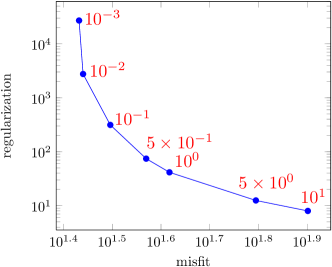
Figure 2: L-curve-based regularization parameter selection. Each point (in blue) on the curve represents the solution of an inverse problem for a different choice of the value of the regularization parameter $\gamma$ (shown in red). For each value of $\gamma$, the vertical axis plots the magnitude of the regularization term $\mathcal{R}(\beta)$ evaluated at the optimum value of $\beta$; the horizontal axis plots the value of the data misfit term i.e., the first term in $\mathcal{J}(\beta)$ defined by (3), also evaluated at the optimum value of $\beta$. The L-curve criterion takes as the “optimum” regularization parameter the value at the point of maximum curvature, in this case $\gamma\approx 0.1$. The criterion posits this value of $\gamma$ as the best tradeoff between minimizing the data misfit and controlling small-scale variations due to data noise in the resulting $\beta$ field.

Figure 3 depicts the solution of the ice sheet inverse problem, i.e., the reconstruction of the Antarctic basal sliding parameter field $\beta$ from InSAR observations of surface ice flow velocity and the nonlinear Stokes ice flow model. Note that the basal sliding parameter field varies over nine orders of magnitude. Low (red) and high (blue) values of $\beta$ represent low and high resistance to basal sliding and correlate with fast and slow ice flow, respectively. As can be seen, weak resistance to basal sliding extends deep into the interior of the continent.

Figure 4 addresses the question of how successful the inversion is in creating a model that explains the data. The top image portrays the observed surface velocity field over the continent, which varies widely from a few meters per year in the interior of the continent (in dark blue), to several kilometers per year in the fast flowing ice streams and outlet glaciers (in bright red). The bottom image shows the surface velocity field that has been reconstructed from solution of the nonlinear Stokes ice flow model using the inferred basal sliding parameter field. By visual inspection, we can see that the two surface velocity fields agree well, particularly in fast flow regions. The difference between the two images reflects the ill-posed nature of the inverse problem, for which data noise and model inadequacy can amplify errors in poorly-inferred features of the inversion parameter field. Nevertheless, the inversion is successful in inferring a basal sliding parameter field and resulting ice sheet model that is able to fit the data well, particularly in the critical regions of the ice sheet that impact sea level (i.e., the fast flowing ice streams of marine ice sheets that deliver the bulk of the mass flux to the ocean, and are most sensitive to forcing changes at ice-ocean interfaces [42]).

Figure 3: Solution of inverse problem of inferring the Antarctic basal sliding parameter field from InSAR surface velocity observations. For visualization purposes, the cube root of the exponential of the basal sliding coefficient is plotted; the actual Robin coefficient $\exp(\beta)$ of the basal sliding boundary condition varies over nine orders of magnitude. Low (red) and high (blue) values for the basal sliding parameter represent low and high resistance to sliding, and correlate with fast and slow ice flow regions, respectively.

Figure 4: Observed (top) and reconstructed via solution of the inverse problem (bottom) surface velocity fields. In the top image, we also highlight the names and locations of the largest ice shelves, the extensions of the ice sheet onto the ocean. Most of the mass from the fast flowing ice streams contributes to ice shelves, and this mass is, over time, released to the ocean due to melting and iceberg calving.

Despite this success in fitting the data, ultimately we are still dealing with an ill-posed inverse problem in which the “true solution” cannot be found exactly. The question we must address is: what confidence do we have in the inverse solution we have obtained? The deterministic inverse problem described in this section is not equipped to answer this question. Instead, we turn to the framework of Bayesian inference, which provides a systematic means of quantifying uncertainty in the solution of the inverse problem. In the next section we present algorithms for making the Bayesian framework tractable for large-scale ice sheet inverse problems.

4 Bayesian quantification of parameter uncertainty: estimating the posterior pdf of the basal sliding parameter field

In this section we tackle the problem of quantifying the uncertainty in the solution of the ice sheet inverse problem discussed in the previous section. We adopt the framework of Bayesian inference [43, 44], and in particular its extension to infinite-dimensional inverse problems [37]. To keep our discussion compact, we begin by presenting finite-dimensional expressions (i.e., after discretization of the parameter space) for the Bayesian formulation of the inverse problem; we refer the reader to [6] for elaboration of the infinite-dimensional framework and associated discretization issues for the ice sheet inverse problem. Next we discuss a low-rank-based approximation of the posterior covariance (built on a low-rank approximation of the Hessian of the data misfit) that permits very large parameter dimensions. We then present expressions that show how the low-rank approximation of this Hessian can be computed for the ice sheet inverse problem, and discuss properties of the Hessian that, in combination with the proposed algorithm, permit computation of the uncertainty in the inverse solution in a fixed number of forward/adjoint solves, independent of the parameter dimension. Finally, the methodology is applied to the large-scale Antarctic ice sheet inverse problem.

4.1 Bayesian solution of the inverse problem

In the Bayesian formulation, we state the inverse problem as a problem of statistical inference over the space of uncertain parameters, which are to be inferred from data and a physical model. The resulting solution to the statistical inverse problem is a posterior distribution that assigns to any candidate set of parameter fields our belief (expressed as a probability) that a member of this candidate set is the “true” parameter field that gave rise to the observed data. When discretized, this infinite-dimensional inverse problem leads to a large-scale problem of inference over the discrete parameters $\boldsymbol{\beta}\in\mathbb R^{n}$, corresponding to degrees of freedom in the parameter field mesh.

The posterior probability distribution combines the prior pdf $\pi_{\text{prior}}(\boldsymbol{\beta})$ over the parameter space, which encodes any knowledge or assumptions about the parameter space that we may wish to impose before the data are considered, with a likelihood pdf $\pi_{\text{like}}(\boldsymbol{d}_{\text{obs}}|\boldsymbol{\beta})$, which explicitly represents the probability that a given set of parameters $\boldsymbol{\beta}$ might give rise to the observed data $\boldsymbol{d}_{\text{obs}}\in\mathbb{R}^{m}$. Bayes’ Theorem then states the posterior pdf explicitly as

$$\pi_{\text{post}}(\boldsymbol{\beta}|\boldsymbol{d}_{\rm{obs}})\propto\pi_{\text{prior}}(\boldsymbol{\beta})\pi_{\text{like}}(\boldsymbol{d}_{\rm{obs}}|\boldsymbol{\beta}).$$ (10)

Note that the infinite-dimensional analog of (10) cannot be stated using pdfs but requires Radon-Nikodym derivatives [37].

For many problems, it is reasonable to choose the prior distribution to be Gaussian. If the parameters represent a spatial discretization of a field, the prior covariance operator usually imposes smoothness on the parameters. This is because rough components of the parameter field are typically not observable from the data and must be determined by the prior to result in a well-posed Bayesian inverse problem. Here, we use elliptic PDE operators to construct the prior covariance, which allows us to build on fast, optimal complexity solvers. More precisely, the prior covariance operator is the inverse of the square of the Laplacian-like operator (5), namely $\mathcal{C}_{\text{\tiny{prior}}}:=\mathcal{A}^{-2}=(-\gamma\boldsymbol{\Delta}_{\Gamma}+\delta I)^{-2}$, where $\gamma$, $\delta>0$ control the correlation length and the variance of the prior operator. This choice of prior ensures that $\mathcal{C}_{\text{\tiny{prior}}}$ is a trace-class operator, guaranteeing bounded pointwise variance and a well-posed infinite-dimensional Bayesian inverse problem [37, 45].

The difference between the observables predicted by the model and the actual observations $\boldsymbol{d}_{\rm{obs}}$ (velocity observations on the ice sheet’s surface) is due to both measurement and model errors, and is represented by the independent and identically distributed Gaussian random variable “noise” vector $\boldsymbol{e}=\boldsymbol{f}(\boldsymbol{\beta})-\boldsymbol{d}_{\text{obs}}\in\mathbb{R}^{m},$ where $\boldsymbol{f}(\cdot)$ is the (generally nonlinear) operator mapping model parameters to output observables. Evaluation of the parameter-to-observable map $\boldsymbol{f}(\boldsymbol{\beta})$ requires solution of the nonlinear Stokes ice flow equations (1) followed by extraction of the surface ice flow velocity field, i.e., it is a discretization of $\mathcal{B}\boldsymbol{u}(\beta)$ in (3). Restating Bayes’ theorem with Gaussian noise and prior, we obtain the statistical solution of the inverse problem, $\pi_{\text{post}}(\boldsymbol{\beta})$, as

$$\pi_{\text{post}}(\boldsymbol{\beta})\propto\exp\Big{(}-\frac{1}{2}\|\boldsymbol{f}(\boldsymbol{\beta})-\boldsymbol{d}_{\text{obs}}\|^{2}_{\boldsymbol{\Gamma}_{\text{noise}}^{-1}}-\frac{1}{2}\|\boldsymbol{\beta}-{\boldsymbol{\beta}}_{\mbox{\tiny prior}}\|^{2}_{\boldsymbol{\Gamma}_{\text{prior}}^{-1}}\Big{)},$$ (11)

where ${\boldsymbol{\beta}}_{\mbox{\tiny prior}}$ is the mean of the prior distribution, $\boldsymbol{\Gamma}_{\text{prior}}\in\mathbb{R}^{n\times n}$ is the covariance matrix for the prior that arises upon discretization of $\mathcal{C}_{\text{\tiny{prior}}}$, and $\boldsymbol{\Gamma}_{\text{noise}}\in\mathbb{R}^{m\times m}$ is the covariance matrix for the noise, which takes over the role of the scaling matrix $\boldsymbol{\Gamma}$ from the deterministic formulation presented in section 3.2.

As is clear from the expression (11), despite the choice of Gaussian prior and noise probability distributions, the posterior probability distribution need not be Gaussian, due to the nonlinearity of $\boldsymbol{f}(\boldsymbol{\beta})$. The non-Gaussianity of the posterior poses challenges for computing statistics of interest for typical large-scale inverse problems, since $\pi_{\text{post}}$ is often a surface in high dimensions, and evaluating each point on this surface requires the solution of the forward model. Numerical quadrature to compute the mean and covariance matrix, for example, is completely out of the question. The method of choice is Markov chain Monte Carlo (MCMC), which judiciously samples the posterior so that sample statistics can be computed. But the use of MCMC for large-scale inverse problems is still prohibitive for expensive forward problems (such as those governed by the nonlinear PDEs of ice sheet flow) and high dimensional parameter spaces (such as the $O(10^{5}-10^{6})$ parameters characterizing the basal sliding parameter field), since even for modest numbers of parameters, the number of samples required can be in the millions (see for example the discussion in [6, 46]). The need to execute millions of forward ice sheet model simulations is simply not feasible, even with today’s multi-petaflops systems.

We are thus led to make a quadratic approximation of the negative log of the posterior (11), which results in a Gaussian approximation of the posterior $\mathcal{N}(\boldsymbol{{\beta}_{\mbox{\tiny MAP}}},\boldsymbol{\Gamma}_{\!\mbox{\tiny post}})$. The mean of this posterior distribution, $\boldsymbol{{\beta}_{\mbox{\tiny MAP}}}$, is the parameter vector maximizing the posterior (11), and is known as the maximum a posteriori (MAP) point. It can be found by minimizing the negative log of (11), which amounts to solving the optimization problem (3) (i.e., the deterministic inverse problem) with appropriately weighted norms, i.e.,

$$\boldsymbol{{\beta}_{\mbox{\tiny MAP}}}:=\underset{\boldsymbol{\beta}}{\arg\min}\Big{(}-\frac{1}{2}\|\boldsymbol{f}(\boldsymbol{\beta})-\boldsymbol{d}_{\text{obs}}\|^{2}_{\boldsymbol{\Gamma}_{\text{noise}}^{-1}}-\frac{1}{2}\|\boldsymbol{\beta}-{\boldsymbol{\beta}}_{\mbox{\tiny prior}}\|^{2}_{\boldsymbol{\Gamma}_{\text{prior}}^{-1}}\Big{)}.$$ (12)

The posterior covariance matrix $\boldsymbol{\Gamma}_{\!\mbox{\tiny post}}$ is then given by the inverse of the Hessian matrix of $\mathcal{J}$ at $\boldsymbol{{\beta}_{\mbox{\tiny MAP}}}$, namely

$$\boldsymbol{\Gamma}_{\!\mbox{\tiny post}}=\left(\boldsymbol{H}_{\mbox{\tiny misfit}}(\boldsymbol{{\beta}_{\mbox{\tiny MAP}}})+\boldsymbol{\Gamma}_{\!\mbox{\tiny prior}}^{-1}\right)^{-1},$$ (13)

where the Hessian of the misfit is given by

$$\boldsymbol{H}_{\mbox{\tiny misfit}}:={\boldsymbol{F}}^{*}\boldsymbol{\Gamma}_{\!\mbox{\tiny noise}}^{-1}{\boldsymbol{F}}-{\boldsymbol{F}}^{*}{\boldsymbol{W}}_{\!u\beta}-{\boldsymbol{W}}_{\!\beta u}{\boldsymbol{F}}+{\boldsymbol{W}}_{\!\beta\beta}.$$ (14)

Here ${\boldsymbol{F}}$ is the Jacobian matrix of the parameter-to-observable map evaluated at ${\boldsymbol{\beta}}_{\mbox{\tiny MAP}}$, ${\boldsymbol{F}}^{*}$ is its adjoint, and ${\boldsymbol{W}}_{\!u\beta}$, ${\boldsymbol{W}}_{\!\beta u}$, and ${\boldsymbol{W}}_{\!\beta\beta}$ involve second derivatives of the negative log posterior with respect to the parameters and the states (explicit expressions for the ice sheet inverse problem will be given below). The Gaussian approximation will be accurate when the parameter-to-observable map $\boldsymbol{f}(\boldsymbol{\beta})$ behaves nearly linearly over the support of the posterior. This will be the case not only when $\boldsymbol{f}(\boldsymbol{\beta})$ is weakly nonlinear, but also for directions in parameter space that are poorly informed by the data (in which case $\boldsymbol{f}(\boldsymbol{\beta})$ is approximately constant and thus the prior dominates), as well as directions in parameter space that are strongly informed by the data (in which case the posterior variance is small and thus the linearization of $\boldsymbol{f}(\boldsymbol{\beta})$ is accurate over the support of the posterior). For the present work, in which we tackle a massive scale Bayesian inverse problem ($\sim 10^{6}$ parameters) governed by large-scale ice sheet flow in Antarctica, all known MCMC methods will be prohibitive, so we cannot compare our Hessian-at-the-MAP-based Gaussian approximation with full sampling of the posterior. However, in [6], we compare this Gaussian approximation with several variants of MCMC sampling of the posterior for a model 2D ice flow problem with a moderate number of parameters ($\sim$100), and conclude that the Hessian-based Gaussian approximation can be appropriate, both as a proposal for MCMC, as well as a stand-alone approximation of the posterior.

4.2 Low-rank based posterior covariance approximation

As stated above, the Gaussian approximation of the posterior (11), with covariance matrix $\boldsymbol{\Gamma}_{\!\mbox{\tiny post}}$ (13) that involves the Hessian of the data misfit evaluated at the MAP point (14), is still intractable. The primary difficulty is that the large parameter dimension $n$ prevents any representation of the posterior covariance $\boldsymbol{\Gamma}_{\!\mbox{\tiny post}}$ as a dense operator. In particular, the Jacobian of the parameter-to-observable map, ${\boldsymbol{F}}$, is formally a dense matrix, and requires $n$ forward PDE solves to construct explicitly. This is intractable when $n$ is large and the forward PDEs are expensive, as in our case of Antarctic ice sheet flow. However, a key feature of the operator ${\boldsymbol{F}}$ is that its action on a (parameter field-like) vector can be formed by solving a (linearized) forward PDE problem; similarly, the action of its adjoint ${\boldsymbol{F}}^{*}$ on a (observation-like) vector can be formed by solving a (linearized) adjoint PDE. Moreover, for many ill-posed inverse problems, the Hessian matrix of the data misfit term in (3), given by (14), is a discretization of a compact operator, i.e., its eigenvalues collapse to zero. This can be understood intuitively, since only the modes of the parameter field that strongly influence the ice velocity are present in the dominant spectrum of (14). In many ill-posed inverse problems, numerous modes of the parameter field (for example, highly oscillatory ones) will have negligible effect on the observables. The range space thus is effectively finite-dimensional even before discretization (and therefore independent of any mesh), and the eigenvalues decay, often rapidly, to zero. Figure 5 illustrates the rapid spectral decay of the data misfit Hessian stemming from our Antarctic ice sheet inverse problem, demonstrating that only about 5,000 (out of 1,190,403) modes of the basal sliding parameter field can be inferred from the data (on the fine mesh). Next we exploit this low-rank structure and the ability to form matrix-free Hessian actions to construct scalable algorithms to approximate the posterior covariance operator.

Rearranging the expression for $\boldsymbol{\Gamma}_{\!\mbox{\tiny post}}$ in (13) to factor out $\boldsymbol{\Gamma}_{\!\mbox{\tiny prior}}$ gives

$$\boldsymbol{\Gamma}_{\!\mbox{\tiny post}}=\left(\boldsymbol{\Gamma}_{\!\mbox{\tiny prior}}\boldsymbol{H}_{\mbox{\tiny misfit}}+\boldsymbol{I}\right)^{-1}\boldsymbol{\Gamma}_{\!\mbox{\tiny prior}}.$$ (15)

This factorization exposes the prior-preconditioned Hessian of the data misfit,

$$\boldsymbol{\tilde{H}}_{\mbox{\tiny misfit}}:=\boldsymbol{\Gamma}_{\!\mbox{\tiny prior}}\boldsymbol{H}_{\mbox{\tiny misfit}}.$$ (16)

Note that $\boldsymbol{\tilde{H}}_{\mbox{\tiny misfit}}$ is symmetric with respect to the inverse prior-weighted inner product. If a square root of $\boldsymbol{\Gamma}_{\!\mbox{\tiny prior}}$ is available, one can alternatively use a symmetric preconditioning of the data misfit Hessian by the prior covariance operator [47, 45]. This results in a prior-preconditioned data misfit Hessian that is symmetric with respect to the Euclidean inner product.

To construct a low-rank approximation of $\boldsymbol{\tilde{H}}_{\mbox{\tiny misfit}}$, we consider the generalized eigenvalue problem

$$\boldsymbol{H}_{\mbox{\tiny misfit}}\boldsymbol{W}=\boldsymbol{\Gamma}_{\!\mbox{\tiny prior}}^{-1}\boldsymbol{W}\boldsymbol{\Lambda},$$ (17)

where $\boldsymbol{\Lambda}=\operatorname{diag}(\lambda_{i})\in\mathbb{R}^{n\times n}$ contains the generalized eigenvalues and the columns of $\boldsymbol{W}\in\mathbb R^{n\times n}$ the generalized eigenvectors. Because $\boldsymbol{\Gamma}_{\!\mbox{\tiny prior}}$ is symmetric positive definite and $\boldsymbol{H}_{\mbox{\tiny misfit}}$ is symmetric positive semi-definite, $\boldsymbol{\Lambda}$ is non-negative and $\boldsymbol{W}$ is orthogonal with respect to $\boldsymbol{\Gamma}_{\!\mbox{\tiny prior}}^{-1}$, so we can scale $\boldsymbol{W}$ so that $\boldsymbol{W}^{T}\boldsymbol{\Gamma}_{\!\mbox{\tiny prior}}^{-1}\boldsymbol{W}=\boldsymbol{I}$. Defining $\boldsymbol{V}:=\boldsymbol{\Gamma}_{\!\mbox{\tiny prior}}^{-1}\boldsymbol{W}$, we can rearrange (17) to get

$$\boldsymbol{\Gamma}_{\!\mbox{\tiny prior}}\boldsymbol{H}_{\mbox{\tiny misfit}}=\boldsymbol{W}\boldsymbol{\Lambda}\boldsymbol{V}^{T}.$$ (18)

When the generalized eigenvalues $\{\lambda_{i}\}$ decay rapidly, we can extract a low-rank approximation of $\boldsymbol{\tilde{H}}_{\mbox{\tiny misfit}}$ by retaining only the $r$ largest eigenvalues and corresponding eigenvectors,

$$\boldsymbol{\tilde{H}}_{\mbox{\tiny misfit}}\approx\boldsymbol{W}_{r}\boldsymbol{\Lambda}_{r}\boldsymbol{V}_{r}^{T}.$$ (19)

Here, $\boldsymbol{W}_{r}\in\mathbb{R}^{n\times r}$ contains only the $r$ eigenvectors of $\boldsymbol{\tilde{H}}_{\mbox{\tiny misfit}}$ that correspond to the $r$ largest eigenvalues, which are assembled into the diagonal matrix $\boldsymbol{\Lambda}_{r}=\operatorname{diag}(\lambda_{i})\in\mathbb{R}^{r\times r}$, and $\boldsymbol{V}_{r}=\boldsymbol{\Gamma}_{\!\mbox{\tiny prior}}^{-1}\boldsymbol{W}_{r}$.

Here, we use randomized SVD algorithms [48, 49] to construct the approximate spectral decomposition. Their performance is comparable to Krylov methods such as Lanczos, which has been used for low-rank approximations of Hessians in very high dimensions in [47, 45, 50]. Both algorithms require only the action of the Hessian on vectors; we show how to do this for the ice sheet Hessian operator in Section 4.3. However, randomized methods have a significant edge over deterministic methods for large-scale problems, since the required Hessian matrix-vector products are independent of each other, providing asynchronicity and fault tolerance.

Once the low-rank approximation (19) has been constructed, we proceed to obtain the posterior covariance matrix. The Sherman-Morrison-Woodbury formula is employed to perform the inverse in (15),

$$\left(\boldsymbol{\tilde{H}}_{\mbox{\tiny misfit}}+\boldsymbol{I}\right)^{-1}=\boldsymbol{I}-\boldsymbol{W}_{r}\boldsymbol{D}_{r}\boldsymbol{V}_{r}^{T}+\mathcal{O}\left(\sum_{i=r+1}^{n}\frac{\lambda_{i}}{\lambda_{i}+1}\right),$$

where $\boldsymbol{D}_{r}:=\operatorname{diag}(\lambda_{i}/(\lambda_{i}+1))\in\mathbb{R}^{r\times r}$. The last term in this expression captures the error due to truncation in terms of the discarded eigenvalues; this provides a criterion for truncating the spectrum, namely that $r$ is chosen such that $\lambda_{r}$ is small relative to 1. With this low-rank approximation, the final expression for the approximate posterior covariance follows from (15),

$$\boldsymbol{\Gamma}_{\!\mbox{\tiny post}}\approx(\boldsymbol{I}-\boldsymbol{W}_{r}\boldsymbol{D}_{r}\boldsymbol{V}_{r}^{T})\boldsymbol{\Gamma}_{\!\mbox{\tiny prior}}=\boldsymbol{\Gamma}_{\!\mbox{\tiny prior}}-\boldsymbol{W}_{r}\boldsymbol{D}_{r}\boldsymbol{W}_{r}^{T}.$$ (20)

Note that (20) expresses the posterior uncertainty as the prior uncertainty less any information gained from the data, filtered through the prior (as a consequence of choosing the prior-preconditioned data misfit Hessian as the operator whose spectrum is truncated). The retained eigenvectors of the prior-preconditioned data misfit Hessian are those modes in parameter space that are simultaneously well-informed by the data and assigned high probability by the prior. Figure 6 displays several of these eigenvectors. The low rank update of the prior covariance in (20), which is based on the low rank approximation (19) of the prior-preconditioned Hessian of the data misfit, has recently been shown to be the optimal rank-$r$ update with respect to several important loss functions [51].

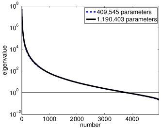
Figure 5: Log-linear plot of spectrum of prior-preconditioned data misfit Hessian for two successively finer parameter/state meshes of the inverse ice sheet problem (12). The curves lie on top of each other, indicating mesh independence of the spectrum. This implies that the dominant eigenvalues/eigenvector of the parameter field—and thus the information content of the data, filtered through the prior—are independent of the parameter dimension. Moreover, since the surface observations are refined with the state mesh, the invariance of the spectrum to mesh refinement also implies that the dominant eigenvalues are independent of the data dimension (once the information content of the data is resolved). The low rank approximation captures this dominant, data-informed portion of the spectrum. The eigenvalues are truncated at 0.2.

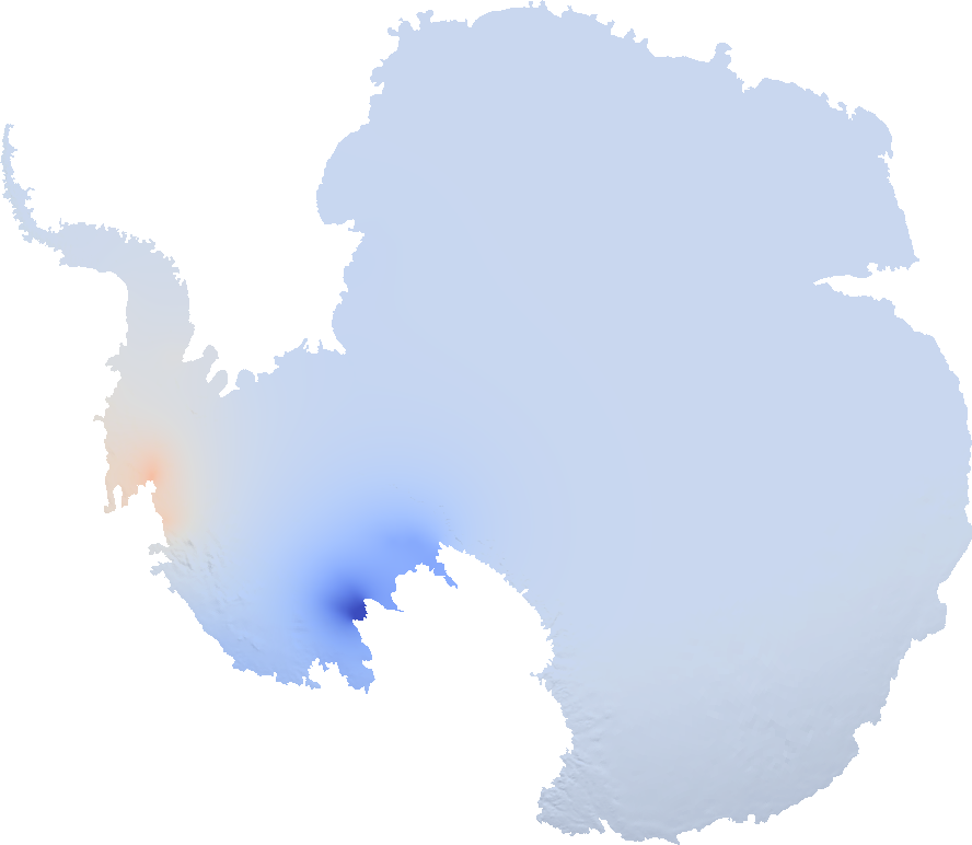
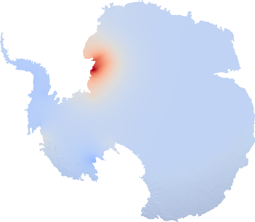
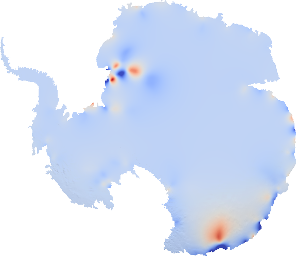
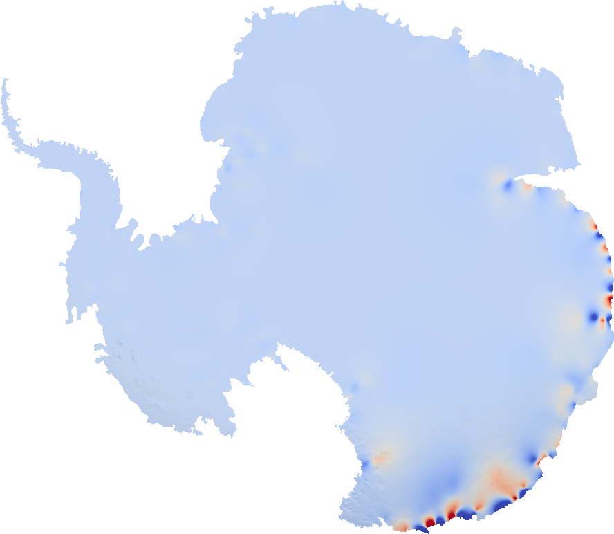
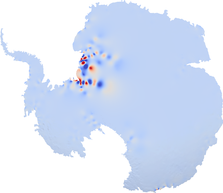
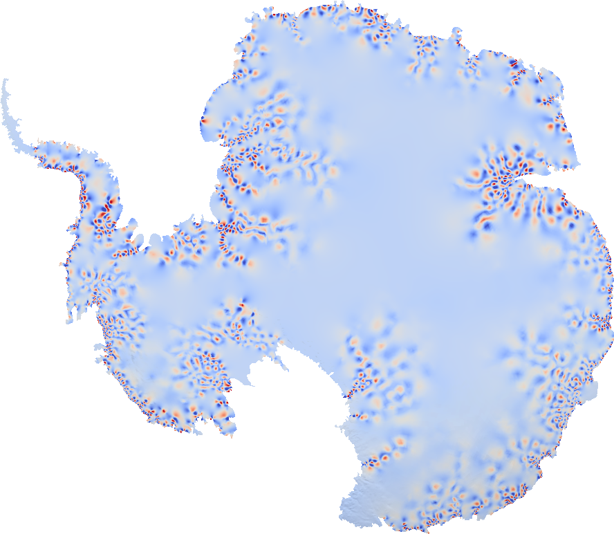
Figure 6: Eigenvectors of the prior-preconditioned data misfit Hessian corresponding (from left to right and top to bottom) to the 1st, 2nd, 100th, 200th, 500th, and 4000th eigenvalues. Note that different eigenvectors localize in different regions of Antarctica, and that eigenvectors corresponding to smaller eigenvalues are increasingly more oscillatory (and thus inform smaller length scales of the basal sliding parameter field) but are also increasingly less informed by the data.

4.3 The action of the Hessian operator

In this section we show that the Hessian-vector products needed in the randomized low-rank algorithms described above can be computed efficiently and matrix-free. The action of the Hessian operator evaluated at a basal sliding parameter field $\beta$ in a direction $\hat{\beta}$ is given by

$$\mathcal{H}(\beta)\hat{\beta} :=\exp(\beta)(\hat{\beta}\boldsymbol{T}\boldsymbol{u}\cdot\boldsymbol{T}\boldsymbol{v}+\boldsymbol{T}\hat{\boldsymbol{u}}\cdot\boldsymbol{T}\boldsymbol{v}+\boldsymbol{T}\boldsymbol{u}\cdot\boldsymbol{T}\hat{\boldsymbol{v}})+\mathcal{A}^{2\kappa}(\hat{\beta}),$$ (21)

where $(\hat{\boldsymbol{u}},\hat{p})$ satisfy a certain linearized forward Stokes equation, which we call the incremental forward Stokes equations

$$\boldsymbol{\nabla}\cdot\hat{\boldsymbol{u}} =\,0 \quad\text{ in }\Omega$$ (22a)

$$-\boldsymbol{\nabla}\cdot\boldsymbol{\sigma}_{\!\hat{\boldsymbol{u}}} =\boldsymbol{0} \quad\text{ in }\Omega$$ (22b)

$$\boldsymbol{\sigma}_{\!\hat{\boldsymbol{u}}}\boldsymbol{n} =\boldsymbol{0} \quad\text{ on }\Gamma_{\!\mbox{\tiny}t}$$ (22c)

$$\hat{\boldsymbol{u}}\cdot\boldsymbol{n} =0 \quad\text{ on }\Gamma_{\!\mbox{\tiny}b}$$ (22d)

$$\boldsymbol{T}\boldsymbol{\sigma}_{\!\hat{\boldsymbol{u}}}\boldsymbol{n}+\exp(\beta)\boldsymbol{T}\hat{\boldsymbol{u}} =-\hat{\beta}\exp(\beta)\boldsymbol{T}\boldsymbol{u} \quad\text{ on }\Gamma_{\!\mbox{\tiny}b},$$ (22e)

with the incremental forward stress

$$\boldsymbol{\sigma}_{\!\hat{\boldsymbol{u}}}:=2\eta(\boldsymbol{u})\,\bigl{(}\mathsf{I}+\frac{1-n}{n}\frac{\dot{\boldsymbol{\varepsilon}}_{\boldsymbol{u}}\otimes\dot{\boldsymbol{\varepsilon}}_{\boldsymbol{u}}}{\dot{\boldsymbol{\varepsilon}}_{\boldsymbol{u}}\cdot\,\dot{\boldsymbol{\varepsilon}}_{\boldsymbol{u}}}\bigr{)}\dot{\boldsymbol{\varepsilon}}_{\hat{\boldsymbol{u}}}-\boldsymbol{I}\hat{p},$$

and $(\hat{\boldsymbol{v}},\hat{q})$ satisfy a linearized version of the adjoint equation, the incremental adjoint Stokes equations

$$\boldsymbol{\nabla}\cdot\hat{\boldsymbol{v}} =\,0 \text{ in }\Omega$$ (23a)

$$-\boldsymbol{\nabla}\cdot\boldsymbol{\sigma}_{\!\hat{\boldsymbol{v}}} =-\boldsymbol{\nabla}\cdot\boldsymbol{\tau}_{\!\hat{\boldsymbol{u}}} \text{ in }\Omega$$ (23b)

$$\boldsymbol{\sigma}_{\!\hat{\boldsymbol{v}}}\boldsymbol{n} =-\mathcal{B}^{*}\boldsymbol{\Gamma}\mathcal{B}\hat{\boldsymbol{u}}-\boldsymbol{\tau}_{\!\hat{\boldsymbol{u}}}\boldsymbol{n} \text{ on }\Gamma_{\!\mbox{\tiny}t}$$ (23c)

$$\hat{\boldsymbol{v}}\cdot\boldsymbol{n} =0 \text{ on }\Gamma_{\!\mbox{\tiny}b}$$ (23d)

$$\boldsymbol{T}\boldsymbol{\sigma}_{\!\hat{\boldsymbol{v}}}\boldsymbol{n}+\exp(\beta)\boldsymbol{T}\hat{\boldsymbol{v}} =-\boldsymbol{T}\boldsymbol{\tau}_{\!\hat{\boldsymbol{u}}}\boldsymbol{n} \text{ on }\Gamma_{\!\mbox{\tiny}b},$$ (23e)

where the incremental adjoint stress $$\boldsymbol{\sigma}_{\!\hat{\boldsymbol{v}}}$$ is given by

$$\boldsymbol{\sigma}_{\!\hat{\boldsymbol{v}}}:=2\eta(\boldsymbol{u})\,\bigl{(}\mathsf{I}+\frac{1-n}{n}\frac{\dot{\boldsymbol{\varepsilon}}_{\boldsymbol{u}}\otimes\dot{\boldsymbol{\varepsilon}}_{\boldsymbol{u}}}{\dot{\boldsymbol{\varepsilon}}_{\boldsymbol{u}}\cdot\,\dot{\boldsymbol{\varepsilon}}_{\boldsymbol{u}}}\bigr{)}\dot{\boldsymbol{\varepsilon}}_{\hat{\boldsymbol{v}}}-\boldsymbol{I}\hat{q},$$

and $$\boldsymbol{\tau}_{\!\hat{\boldsymbol{u}}}=2\eta(\boldsymbol{u})\Psi\dot{\boldsymbol{\varepsilon}}_{\hat{\boldsymbol{u}}}$$, where

$$\Psi :=\frac{1-n}{n}\biggr{[}\frac{\dot{\boldsymbol{\varepsilon}}_{\boldsymbol{u}}\otimes\dot{\boldsymbol{\varepsilon}}_{\boldsymbol{v}}+\dot{\boldsymbol{\varepsilon}}_{\boldsymbol{v}}\otimes\dot{\boldsymbol{\varepsilon}}_{\boldsymbol{u}}}{\dot{\boldsymbol{\varepsilon}}_{\boldsymbol{u}}\cdot\,\dot{\boldsymbol{\varepsilon}}_{\boldsymbol{u}}}+\frac{\dot{\boldsymbol{\varepsilon}}_{\boldsymbol{u}}\cdot\,\dot{\boldsymbol{\varepsilon}}_{\boldsymbol{v}}}{\dot{\boldsymbol{\varepsilon}}_{\boldsymbol{u}}\cdot\,\dot{\boldsymbol{\varepsilon}}_{\boldsymbol{u}}}\biggl{(}\frac{1-3n}{n}\frac{\dot{\boldsymbol{\varepsilon}}_{\boldsymbol{u}}\otimes\dot{\boldsymbol{\varepsilon}}_{\boldsymbol{u}}}{\dot{\boldsymbol{\varepsilon}}_{\boldsymbol{u}}\cdot\,\dot{\boldsymbol{\varepsilon}}_{\boldsymbol{u}}}+\mathsf{I}\biggr{)}\biggr{]}.$$

We see that the incremental forward and incremental adjoint Stokes equations are linearized versions of their forward and adjoint counterparts, having the same (linearized) operator and differing only in the source terms. Thus, computation of Hessian actions on vectors amount to solution of a pair of forward/adjoint (linearized) Stokes equations, similar to the computation of the gradient. Since the gradient and Hessian action require just one and two linearized Stokes solves, respectively, they are significantly cheaper to evaluate than solving the (nonlinear) forward problem, which typically requires an order of magnitude more linearized Stokes solves.

4.4 Scalability of Bayesian solution of the inverse problem

We now discuss the overall scalability of our algorithms for Bayesian solution of the inverse problem. First, we characterize the scalability of construction of the low-rank-based approximate posterior covariance matrix in (20). As stated before, the parameter-to-observable map ${\boldsymbol{F}}$ cannot be constructed explicitly, since it requires $n$ linearized forward Stokes solves. However, as elaborated above, its action on a vector can be computed by a single linearized Stokes solve, regardless of the number of parameters $n$ and observations $m$. Similarly, the action of ${\boldsymbol{F}}^{*}$ on a vector can be computed via a linearized adjoint Stokes solve. Moreover, the prior is usually much cheaper to apply than a forward/adjoint solve (here, it is a scalar elliptic solve on the basal boundary). Therefore, the cost of applying $\boldsymbol{\tilde{H}}_{\mbox{\tiny misfit}}$ to a vector—and thus the per iteration cost of the randomized SVD algorithm—is dominated by a pair of linearized forward and adjoint Stokes solves.

The randomized SVD algorithm requires a number of matrix-vector products proportional to the effective rank $r$ of the matrix [49, 48]. Thus, the remaining component to establish scalability of the low-rank approximation of $\boldsymbol{\tilde{H}}_{\mbox{\tiny misfit}}$ is independence of $r$—and therefore the number of matrix-vector products, and hence Stokes solves—from the parameter dimension $n$. This is the case when $\boldsymbol{H}_{\text{misfit}}$ in (14) is a (discretization of a) compact operator, and when preconditioning by $\boldsymbol{\Gamma}_{\!\mbox{\tiny prior}}$ does not destroy the spectral decay. This situation is typical for many ill-posed inverse problems, in which the prior is either neutral or of smoothing type. Hence, a low-rank approximation of $\boldsymbol{\tilde{H}}_{\mbox{\tiny misfit}}$ can be made that does not scale with parameter or data dimension, instead depending only on the information content of the data, filtered through the prior. This is indeed the case for our ice sheet inverse problem, as demonstrated in Figure 5.

Once the $r$ eigenpairs defining the low rank approximation have been computed, estimates of uncertainty can be computed by interrogating $\boldsymbol{\Gamma}_{\!\mbox{\tiny post}}$ in (20) at a cost of just $r$ inner products (which are negligible) plus elliptic solves representing the action of the prior $\boldsymbol{\Gamma}_{\!\mbox{\tiny prior}}$ on a vector (here carried out with an algebraic multigrid solver and therefore algorithmically scalable). For example, samples can be drawn from the Gaussian defined with a covariance $\boldsymbol{\Gamma}_{\!\mbox{\tiny post}}$, a row/column of $\boldsymbol{\Gamma}_{\!\mbox{\tiny post}}$ can be computed, and the action of $\boldsymbol{\Gamma}_{\!\mbox{\tiny post}}$ in a given direction can be formed, all at cost that is $O(rn)$ in the number of inner products in addition to the $O(n)$ cost of the multigrid solve. Moreover, the posterior variance field, i.e., the diagonal of $\boldsymbol{\Gamma}_{\!\mbox{\tiny post}}$, can be found with $O(rn)$ linear algebra plus $O(r)$ multigrid solves.

4.5 Samples from the prior and Gassianized posterior

In this section we provide some results that illustrate the quantification of uncertainty in the solution of the Antarctic ice sheet inverse problem. The number of degrees of freedom was 3,785,889 for each of the discretized state-like variables (state, adjoint, incremental state, and incremental adjoint velocities and pressures) and 409,545 for the uncertain basal sliding parameter field. The problem was solved on 1024 processor cores. We used the Laplacian prior operator with $\kappa=1$, $\gamma=10$, and $\delta=10^{-5}$, and took a zero mean of the basal sliding parameter field, i.e., $\beta_{0}=0$. To characterize the noise, we used a diagonal noise covariance matrix $\boldsymbol{\Gamma}_{\!\mbox{\tiny noise}}$ with entries $\sigma^{i}_{\text{noise}}=0.1(\|\boldsymbol{d}_{\rm{obs}}^{i}\|^{2}+\varepsilon)^{1/2}$ for $i=1,...,m$, with $\varepsilon=10^{-9}$. That is, $\sigma^{i}_{\text{noise}}$ is (at least) 10% of the velocity magnitude at the $i$th observational data point.

To compute the MAP point via solution of the optimization problem (12), 213 (outer) Newton iterations were necessary to decrease the nonlinear residual by a factor of $10^{3}$. In each of these outer Newton iterations, the nonlinear forward Stokes problem has to be solved, for which we use an (inner) Newton method. These inner Newton solves are terminated after the residual is decreased by a factor of $10^{8}$, which takes an average of 5 Newton iterations, each requiring a linearized Stokes solve. In addition to the nonlinear Stokes solve, each (outer) Newton iteration requires computation of the gradient, which costs one linearized Stokes solve, and inexact solution of the (outer) Newton system (6) using CG, which requires a number of Hessian-vector products. The average number of CG iterations per (outer) Newton step was 239. Each Hessian-vector product requires a pair of linearized Stokes solves, one incremental forward and one incremental adjoint. The tolerance for these incremental Stokes solves was set to $10^{-6}$. Altogether, finding the MAP point required a total of 107,578 linear(ized) Stokes solves.

We approximated the covariance matrix at the MAP point via a low-rank representation employing 5,000 products of the Hessian matrix with random vectors; hence, the cost of this approximation is 10,000 incremental forward/adjoint (linearized) Stokes solves. Thus, the cost (measured in Stokes solves) of quantifying the uncertainty in the MAP solution is about an order of magnitude less than that of finding the MAP point.

Figure 7: The posterior mean. Low (red) and high (blue) values for the basal sliding parameter correlate with fast and slow ice flow regions, respectively.

Figure 7 depicts the MAP point, and Figure 8 shows the prior and posterior pointwise standard deviations. One observes that the uncertainty is vastly reduced everywhere in the domain, and that the reduction is greatest along the fast ice flow regions.

Figure 8: This figure shows the standard deviations of the pointwise marginals of the prior distribution (left) and of (the Gaussian approximation of) the posterior distribution (right).

In Figure 9 we show samples (of the basal sliding parameter field) from the prior (top row) and from the Gaussian approximation of the posterior (bottom row) pdf. The difference between the two sets of samples reflects the information gained from the data in solving the inverse problem. The differences in the basal sliding parameter field across the posterior samples demonstrate that in the fast ice flow regions there is small variability, while in the center and in West Antarctica, we observe larger variability in the inferred parameters, reflecting uncertainty due to insensitivity of surface velocities to the basal sliding in slow velocity and small velocity gradient regions.

This uncertainty in the inference of the basal sliding parameter field, however, is merely an intermediate quantity. What is of ultimate interest is predictions of output quantities of interest, with associated uncertainties, using the ice sheet model with inferred parameters and their associated uncertainties, which have been computed using the methods of this section. This is the subject of the next section.

Figure 9: Samples from the prior (top row) and Gaussian approximation of the posterior (bottom row) distributions for the basal sliding parameter field. The difference between the prior and posterior samples reflects the information gained from the observational data. The large scale features of the posterior samples consistently resemble the posterior mean shown in Figure 7. Note the small variability in the fast ice flow regions, while central and West Antarctica exhibit large variability in the inferred basal sliding parameter field.

5 Prediction with quantified uncertainty: forward propagation of basal sliding parameter uncertainty to mass flux prediction

Once the inverse problem to infer the unknown basal sliding parameter field from observed surface velocities has been solved, and the uncertainty in this inference quantified through a Gaussian approximation of the posterior (made tractable by a low-rank representation of the prior-preconditioned data misfit Hessian), we are ready to propagate the uncertain basal sliding parameter field through the ice flow model to yield a prediction of our quantity of interest with associated uncertainty. Ultimately our interest is in predicting the ice mass flux to the ocean several decades in the future, under various climate change scenarios. However, this requires a model of the ice sheet as an evolving body, more mechanistic basal boundary conditions, and coupling to atmosphere and ocean models. In the present work, we have instead chosen to illustrate our data-to-prediction framework with a simpler quantity of interest $Q$ given by the ice mass flux to the ocean using the steady state ice sheet model employed in the previous sections. Below, we describe scalable algorithms for this final step of our data-to-prediction framework.

Formally, this amounts to solving a system of stochastic PDEs given by the nonlinear Stokes forward model with the uncertain basal sliding parameter described by a Gaussian random field. While the low rank approximation of Section 4.2 has resulted in significant dimensionality reduction (from $O(10^{6})$ to $O(10^{3})$, as seen in Figure 5), the effective dimension, $\sim$4000, is still large in absolute terms. Given that this many modes in parameter space are required to quantify the uncertainty in the basal sliding coefficient parameters, and given the expense of solving the large-scale highly-nonlinear forward ice sheet flow problem, the use of Monte Carlo sampling methods would be prohibitive, since millions of forward solves would likely be required to characterize the statistics of the prediction quantity. Similarly, for the problem we target, the use of polynomial chaos methods would be prohibitive due to the curse of dimensionality that afflicts such methods.

Instead, consistent with our Gaussian approximation of the Bayesian solution of the inverse problem, and our desire to scale to very large parameter dimensions, here we linearize the parameter-to-prediction map at the MAP point, resulting in a Gaussian approximation of the prediction pdf, $\mathcal{N}(Q_{\text{\tiny MAP}},\Gamma_{\!\text{prediction}})$. The mean of this prediction pdf, $Q_{\text{\tiny MAP}}$, is computed by solving the forward ice sheet flow model (1) using ${\beta}_{\mbox{\tiny MAP}}$ as the basal sliding parameter, i.e., the MAP point solution of the inverse problem. The covariance operator, $\Gamma_{\!\text{prediction}}$, is found by propagating the covariance of the model parameters (which is given by the inverse of the Hessian evaluated at ${\beta}_{\mbox{\tiny MAP}}$, i.e., $\mathcal{H}^{-1}({\beta}_{\mbox{\tiny MAP}})$), through the linearized parameter-to-prediction map, i.e., by

$$\Gamma_{\!\text{prediction}}:=\mathcal{F}({\beta}_{\mbox{\tiny MAP}})\,\mathcal{H}^{-1}({\beta}_{\mbox{\tiny MAP}})\,\mathcal{F}^{*}({\beta}_{\mbox{\tiny MAP}}),$$ (24)

where $\mathcal{F}({\beta}_{\mbox{\tiny MAP}})$ is the Jacobian of the parameter-to-prediction map, evaluated at the MAP point ${\beta}_{\mbox{\tiny MAP}}$, and the Hessian at the MAP, $\mathcal{H}({\beta}_{\mbox{\tiny MAP}})$, is defined by its action in a direction by (21), which involves solution of the incremental forward (22) and incremental adjoint (23) Stokes problems.

One of the key ideas to enabling scalability of the prediction-under-uncertainty problem is that the Jacobian of the parameter-to-prediction map $\mathcal{F}({\beta}_{\mbox{\tiny MAP}})$ can be determined for each prediction quantity $Q$ by computing the gradient of $Q$ with respect to the parameter field $\beta$. In our case, we are interested in using the steady state ice flow model to predict the net ice mass flux into the ice shelves, and eventually into the ocean,

$$Q(\beta):=\int_{\Gamma_{o}}\!\!\rho\boldsymbol{u}(\beta)\cdot\boldsymbol{n}\,ds,$$ (25)

where $\Gamma_{o}$ is an outflow boundary of interest. The gradient of $Q$ with respect to $\beta$ evaluated at ${\beta}_{\mbox{\tiny MAP}}$ can then be found as follows. First, solve the forward problem (1) with basal sliding parameter field given by ${\beta}_{\mbox{\tiny MAP}}$. Then, solve an adjoint problem defined for the quantity $Q$, i.e.,

$$\boldsymbol{\nabla}\cdot\boldsymbol{v} =0 \quad\text{ in }\Omega$$ (26a)

$$-\boldsymbol{\nabla}\cdot\boldsymbol{\sigma}_{\!\boldsymbol{v}} =\boldsymbol{0} \quad\text{ in }\Omega$$ (26b)

$$\boldsymbol{\sigma}_{\!\boldsymbol{v}}\boldsymbol{n} =0 \quad\text{ on }\Gamma_{\!\mbox{\tiny}t}$$ (26c)

$$\boldsymbol{\sigma}_{\!\boldsymbol{v}}\boldsymbol{n} =-\rho\boldsymbol{n} \quad\text{ on }\Gamma_{\!\mbox{\tiny}o}$$ (26d)

$$T\boldsymbol{\sigma}_{\!\boldsymbol{v}}\boldsymbol{n}+\exp({\beta}_{\mbox{\tiny MAP}})\boldsymbol{T}\boldsymbol{v} =\boldsymbol{0},\;\;\boldsymbol{v}\cdot\boldsymbol{n}=0 \quad\text{ on }\Gamma_{\!\mbox{\tiny}b}$$ (26e)

where the adjoint stress is given by (9). Since we are using the same ice flow model for the prediction problem that was used to infer $\beta$, the adjoint problem (26) for $Q$ resembles the adjoint problem for the regularized data misfit functional $\mathcal{J}$ in (3), but with a different source term given by the variation of $Q$ with respect to the state variables $(\boldsymbol{u},p)$. This means that the adjoint Stokes solver can be reused for this purpose (which in turn is the same as the linearized forward Stokes solver). Once the forward velocity $\boldsymbol{u}$ and adjoint velocity $\boldsymbol{v}$ are found, $\mathcal{F}({\beta}_{\mbox{\tiny MAP}})$, which is the gradient of $Q$ at ${\beta}_{\mbox{\tiny MAP}}$, can be found from the gradient expression (7) without the regularization term, i.e., from

$$\mathcal{F}({\beta}_{\mbox{\tiny MAP}}):=\exp({\beta}_{\mbox{\tiny MAP}})\;\boldsymbol{T}\boldsymbol{u}\cdot\boldsymbol{T}\boldsymbol{v}\quad\text{ on }\Gamma_{\!\mbox{\scriptsize b}}.$$ (27)

Note that if a different flow model is used for the prediction phase (such as one governing a dynamically evolving ice sheet), then a new adjoint equation and gradient expression will have to be derived for that model for the prediction step.

Now that $\mathcal{F}({\beta}_{\mbox{\tiny MAP}})$ has been found, the next step is to form $\mathcal{H}^{-1}({\beta}_{\mbox{\tiny MAP}})\mathcal{F}^{*}({\beta}_{\mbox{\tiny MAP}})$, which could be found by solving a linear system using the preconditioned CG method described in Section 3.2. This would require a number of forward/adjoint incremental Stokes solves equal to the number of CG iterations. Instead, since $\mathcal{H}^{-1}({\beta}_{\mbox{\tiny MAP}})$ is available in the compact form given by (20) (based on the low-rank approximation of the prior-preconditioned Hessian of the data misfit), the product $\mathcal{H}^{-1}({\beta}_{\mbox{\tiny MAP}})\mathcal{F}^{*}({\beta}_{\mbox{\tiny MAP}})$ can be formed without having to solve incremental Stokes equations, at the cost of just linear algebra (vector scalings, additions and inner products). The final step of the inner product of $\mathcal{F}({\beta}_{\mbox{\tiny MAP}})$ with $\mathcal{H}^{-1}({\beta}_{\mbox{\tiny MAP}})\mathcal{F}^{*}({\beta}_{\mbox{\tiny MAP}})$ is straightforward. The result is the covariance of the ice mass flux $Q$, given uncertainties in the satellite observations of surface velocity, uncertainties in the basal sliding parameter field as inferred from the satellite data, and the ice sheet flow model and corresponding prediction quantity $Q$. <ltx:note>For a single $Q$</ltx:note>, the prediction density $\mathcal{N}(Q_{\text{\tiny MAP}},\Gamma_{\!\text{prediction}})$ is univariate. The cost to obtain this pdf, once the low rank-based inverse Hessian (20) has been computed in the Bayesian inference phase, is just a forward solve followed by an (as always, linear) adjoint solve, i.e., at little cost beyond the forward solve.

Figure 10 provides results of uncertainty propagation from parameters to predictions following the framework outlined above. Recent work on “inference for prediction” has shown that, for linear inverse problems and linear parameter-to-prediction maps, there is a unique direction in parameter space that influences the prediction quantity of interest [52]. Finding this direction involves identifying parameter modes that are both informed by the observational data and also required for estimating the quantity of interest. We adopt the inference-for-prediction (IFP) algorithm presented more generally for multiple quantities of interest in [52]. Denoting the Hessian square root by $\mathcal{G}:=\mathcal{H}^{-1/2}({\beta}_{\mbox{\tiny MAP}})$ and using the linearized parameter-to-prediction map $\mathcal{F}({\beta}_{\mbox{\tiny MAP}})$, we compute the eigendecomposition $\boldsymbol{\Psi}{\Sigma}^{2}\boldsymbol{\Psi}^{*}$ of ${\mathcal{G}}^{*}{\mathcal{F}^{*}({\beta}_{\mbox{\tiny MAP}})}\mathcal{F}({\beta}_{\mbox{\tiny MAP}})\mathcal{G}$. Since this operator has rank 1, the eigenvector $\boldsymbol{\Psi}$ corresponding to the only nonzero eigenvalue is given by ${\mathcal{G}}^{*}{\mathcal{F}^{*}({\beta}_{\mbox{\tiny MAP}})}$, and the corresponding eigenvalue is ${\Sigma}^{2}=\|{\mathcal{G}}^{*}{\mathcal{F}^{*}({\beta}_{\mbox{\tiny MAP}})}\|^{2}$. Following [52], the influential direction for prediction (based on linearizations of the parameter-to-observable map and the parameter-to-prediction map) is given by

$$\mathcal{W}=\mathcal{G}\boldsymbol{\Psi}{\Sigma}^{-1/2}.$$

Using the explicit form of $\boldsymbol{\Psi}$, the influential direction for prediction in the IFP algorithm thus simplifies to $\mathcal{W}=\mathcal{G}{\mathcal{G}}^{*}{\mathcal{F}^{*}({\beta}_{\mbox{\tiny MAP}})}{\Sigma}^{-1/2}={\Sigma}^{-1/2}\mathcal{H}({\beta}_{\mbox{\tiny MAP}})^{-1}\mathcal{F}^{*}({\beta}_{\mbox{\tiny MAP}})$. This direction, or “mode” of the parameter field, is depicted in the bottom row of Figure 10 for ice mass fluxes over three different portions of the outflow boundary (all of Antarctica, just East Antarctica, and just the Totten Glacier). The mean and standard deviation of the prediction probability distribution for the three ice mass fluxes are: 1170.83 $\pm$ 1080.09, 359.60 $\pm$ 1.02, and 71.24 $\pm$ 0.30 Gt/a, respectively. We also computed standard deviations with the prior covariance and, as expected, found larger values, namely 1327.22, 525.24, and 179.73 Gt/a for all of Antarctica, East Antarctica and the Totten Glacier, respectively. The top row of Figure 10 portrays the gradient of $Q$ with respect to $\beta$, computed using (27) for each case; these plots show the regions in parameter space to which $Q$ is most sensitive. Note the differences with the bottom row, which captures not only sensitivity of the prediction quantity to $\beta$ (i.e., the gradient $\mathcal{F}$), but also uncertainty in the $\beta$ field (i.e., $\mathcal{H}^{-1}$). The most uncertain regions are not necessarily the most sensitive, and vice versa. Since, as implied by Figure 9, central and West Antarctica exhibit the largest uncertainties, we expect these regions to play an important role in the parameter modes shown in the bottom row of Figure 10, especially where the sensitivity with respect to the basal sliding parameter is not dominant, e.g., in the bottom left figure. On the other hand, in the center and right figures in the bottom row, focusing on East Antarctica, where the posterior samples suggest lower uncertainties, the modes show mixed uncertainty and sensitivity influence.

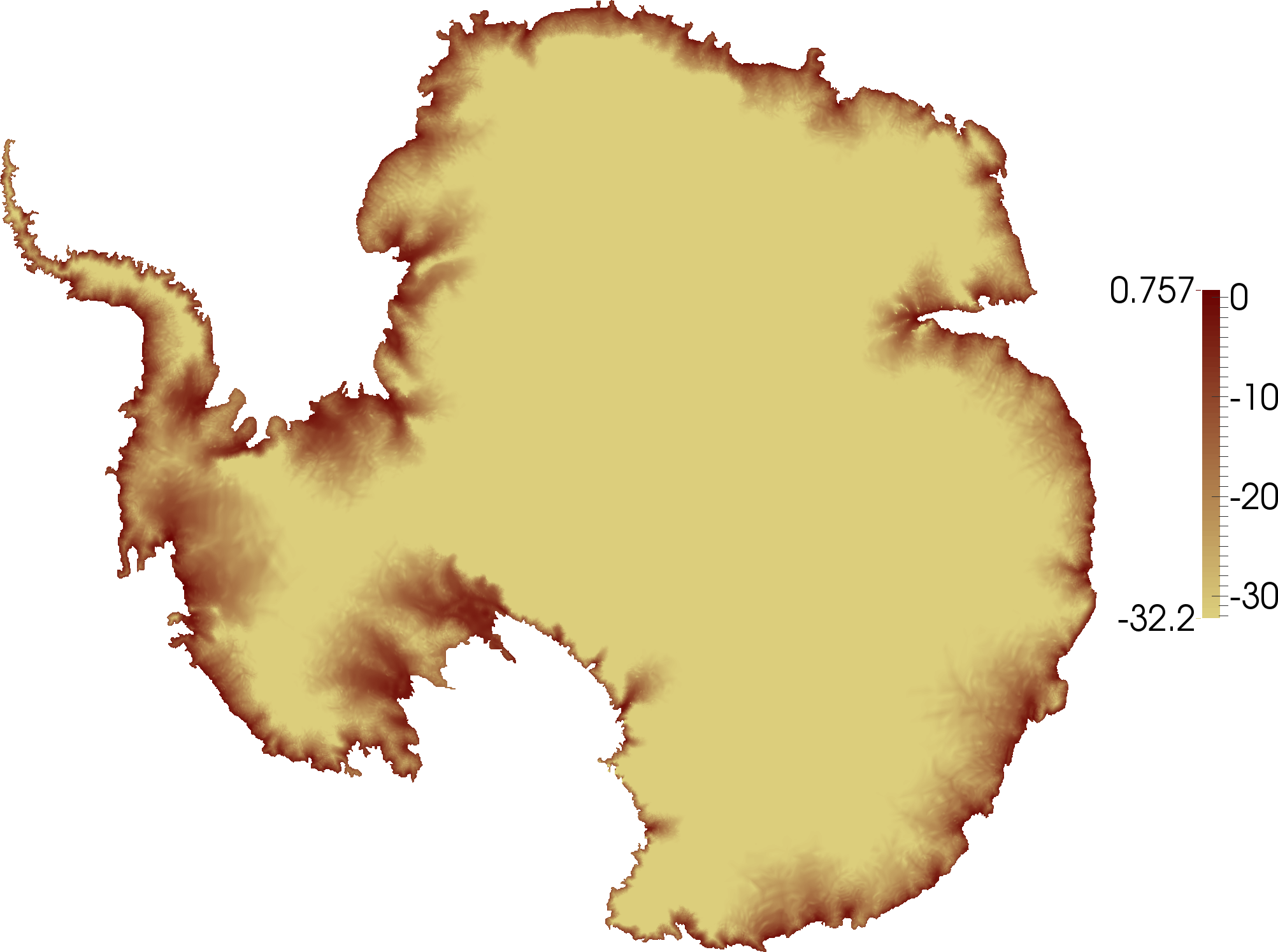
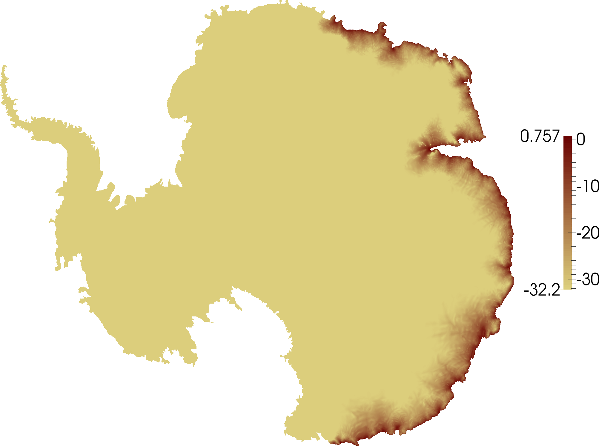
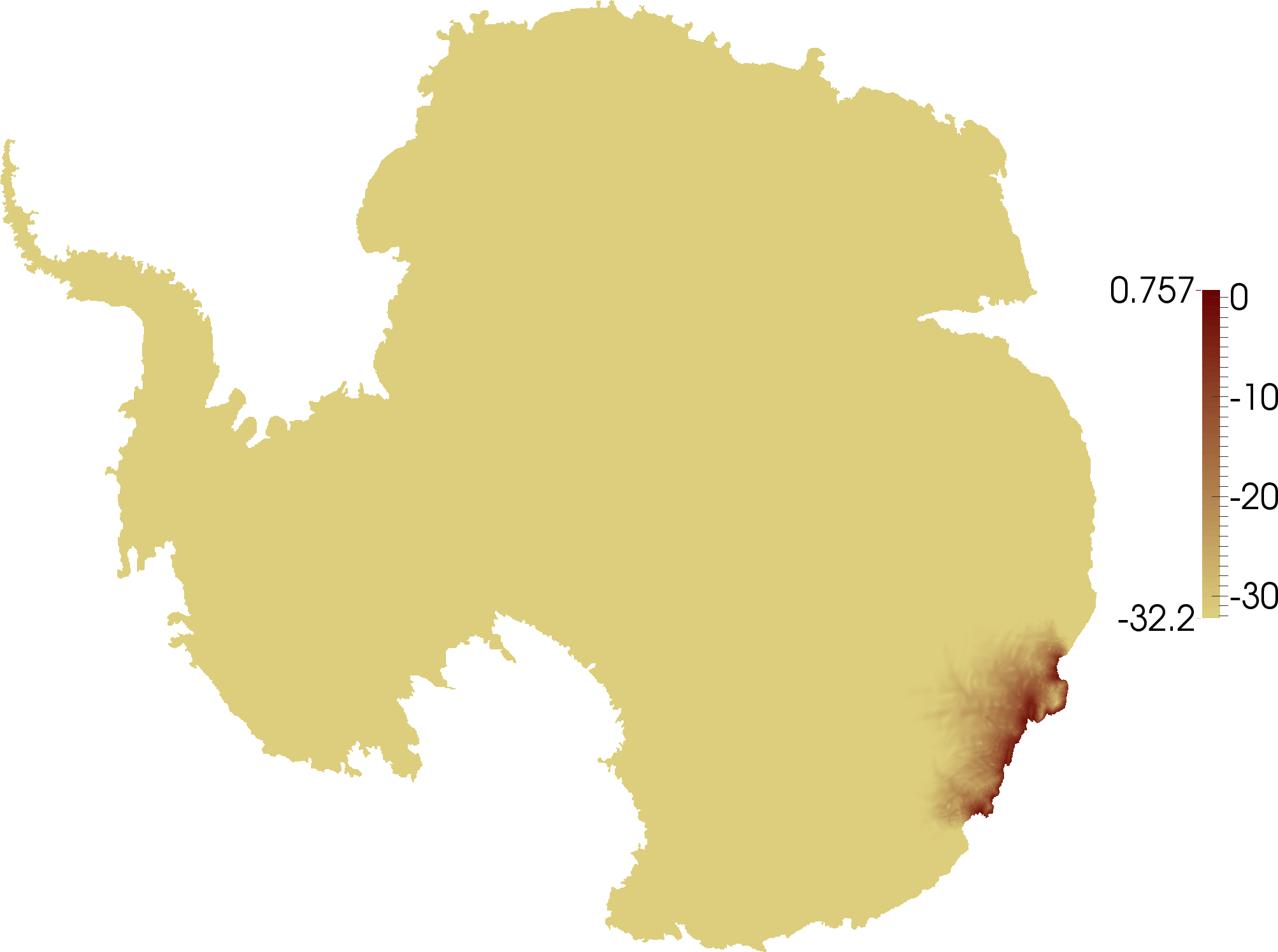
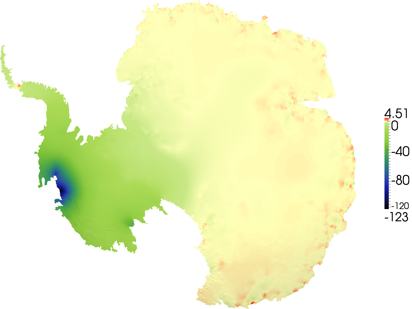
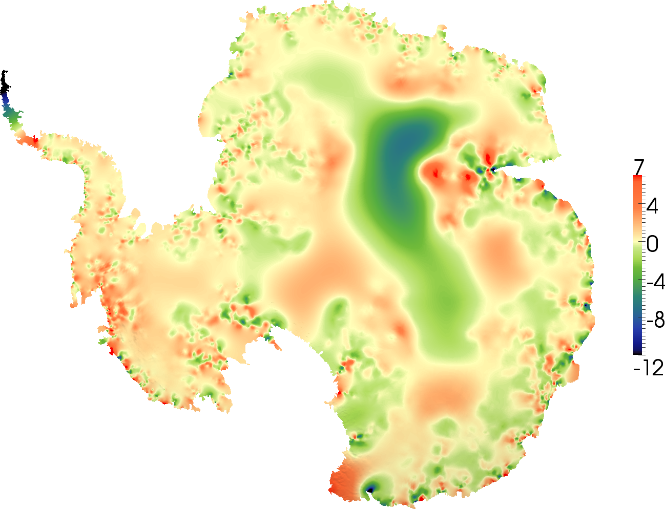
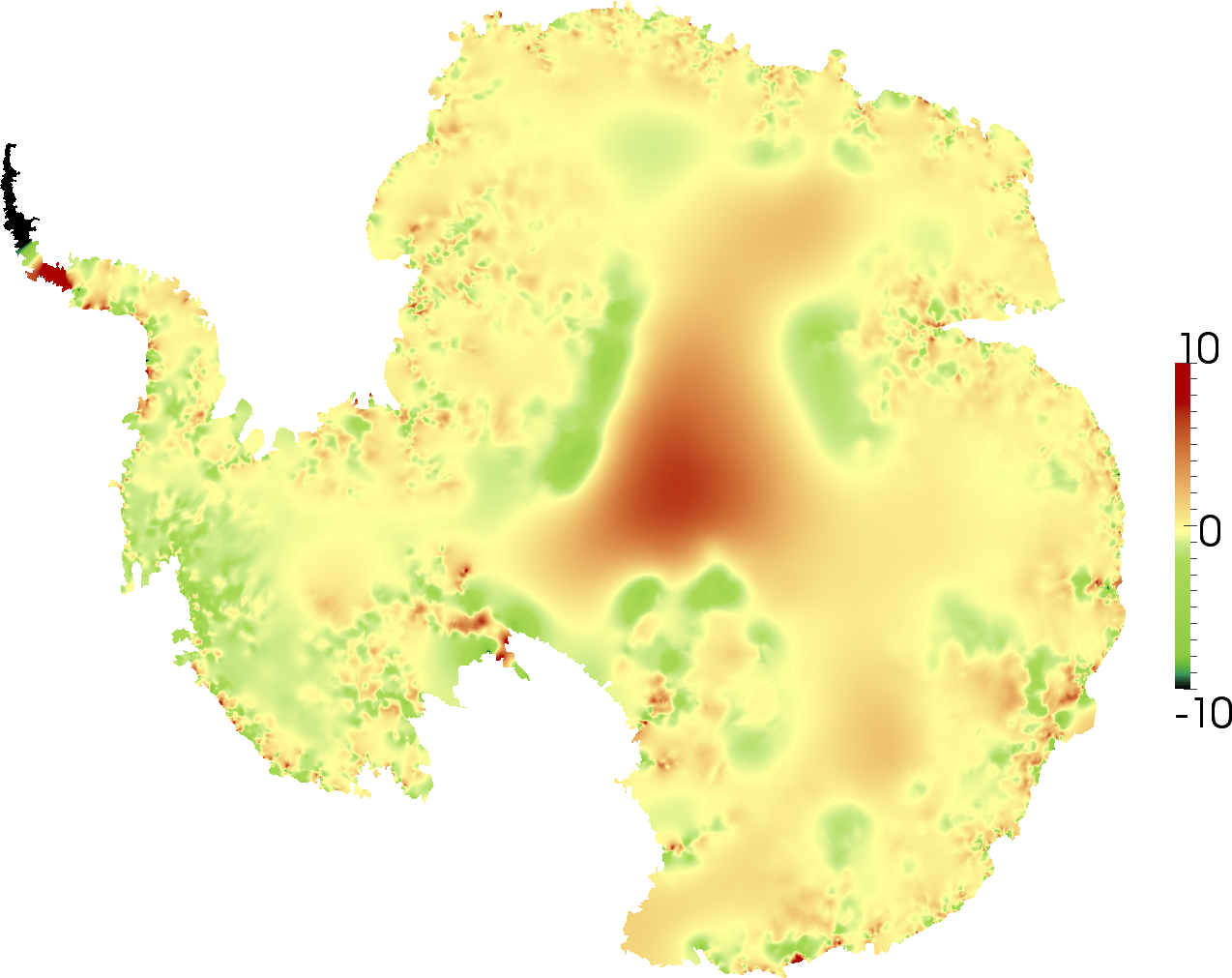
Figure 10: The (logarithm of the) gradient of the prediction quantity $Q$ with respect to the uncertain basal sliding parameter $\beta$ (top row) and the directions that jointly maximize uncertainty and sensitivity for the prediction (bottom row) following [52]. For visualization purposes, in the top row we plot $\ln(|\mathcal{F}({\beta}_{\mbox{\tiny MAP}})|+10^{-10})$. The quantities of interest are the mass flux of ice into the ocean for the entire boundary (left column), for all of East Antarctica (center column), and for the Totten Glacier region (right column). The mean and standard deviation of the prediction probability distribution for the three ice mass fluxes are: 1170.83 $\pm$ 1080.09, 359.60 $\pm$ 1.02, and 71.24 $\pm$ 0.30 Gt/a, respectively.

6 Conclusions

We have presented a scalable framework for solving end-to-end, data-to-prediction problems, presented in the context of the flow of the Antarctic ice sheet, and motivated by prediction of its contribution to sea level. We begin with observational data and associated uncertainty, then infer model parameters from the data (Section 3), quantify uncertainties in the inference of the parameters (Section 4), and finally propagate those uncertain model parameters to yield a prediction quantity of interest with quantified uncertainties (Section 5). We show that the cost of the entire data-to-prediction framework, when measured in forward or adjoint Stokes solves, is a constant independent of the parameter or data dimension. When combined with a scalable forward solver such as that presented in Section 2, this results in a data-to-prediction framework that is independent of the state dimension and number of processor cores as well.

This scalability is a consequence of three properties of the data-to-prediction process and their exploitation by our algorithms: (1) when inferring the parameter field, the data are informative about only a low-dimensional subspace within the high-dimensional parameter space, and thus a Newton-CG optimization method, preconditioned by the regularization operator, converges in a number of Newton and CG iterations that is independent of the parameter and data dimensions, depending only on the information content of the data; (2) when estimating the uncertainty in the inverse solution, the same property dictates that the Hessian of the data misfit admits a low rank representation, and this can be extracted via randomized SVD in a number of matrix-free Hessian-vector products (each of which requires a pair of incremental forward/adjoint Stokes solves) that is also independent of the data and parameter dimensions, and again depends only on the information contained within the data; and (3) when propagating the inferred parameter uncertainties forward through the ice flow model to yield predictions with quantified uncertainties, the prediction pdf can be formed through the action of the inverse Hessian on the gradient of the prediction quantity with respect to the uncertain parameters, which in turn is found through an additional adjoint Stokes solve. Thus, the entire data-to-prediction process is sensitive only to the true information contained within the data, as opposed to the ostensible data or parameter dimensions.

The uncertainty analysis presented here relies on linearizations of the parameter-to-observable and parameter-to-prediction maps, leading to Gaussian approximations of the parameter posterior pdf and prediction quantity of interest pdf. Ultimately one would like to relax these approximations and fully explore the resulting non-Gaussian pdfs; how to do this while retaining scalability for such large-scale complex problems remains an open question, and is a subject of ongoing work.

References

References

- [1] A. Shepherd, E. R. Ivins, A. Geruo, V. R. Barletta, M. J. Bentley, S. Bettadpur, K. H. Brigg, D. H. Bromwich, R. Forsberg, N. Galin, et al., A reconciled estimate of ice-sheet mass balance, Science 338 (6111) (2012) 1183–1189.
- [2] E. Hanna, F. J. Navarro, F. Pattyn, C. M. Domingues, X. Fettweis, E. R. Ivins, R. J. Nicho lls, C. Ritz, B. Smith, S. Tulaczyk, et al., Ice-sheet mass balance and climate change, Nature 498 (7452) (2013) 51–59.
- [3] M. J. O’Leary, P. J. Hearty, W. G. Thompson, M. E. Raymo, J. X. Mitrovica, J. M. Webster, Ice sheet collapse following a prolonged period of stable sea level during the last interglacial, Nature Geoscience 6 (2013) 796–800.
- [4] R. J. Nicholls, S. Hanson, C. Herweijer, N. Patmore, S. Hallegatte, J. Corfee-Morlot, J. Château, R. Muir-Wood, Ranking port cities with high exposure and vulnerability to climate extremes: Exposure estimates, OECD Environment Working Papers, No. 1, OECD Publishing (2008). doi:10.1787/011766488208.
- [5] Climate change 2007: Impacts, adaptation, and vulnerability. Contribution of working group II to the fourth assessment report of the intergovernmental panel on climate change, Cambridge University Press, Cambridge, United Kingdom (2007).
- [6] N. Petra, J. Martin, G. Stadler, O. Ghattas, A computational framework for infinite-dimensional Bayesian inverse problems: Part II. Stochastic Newton MCMC with application to ice sheet inverse problems, SIAM Journal on Scientific Computing 36 (4) (2014) A1525–A1555.
- [7] T. Isaac, G. Stadler, O. Ghattas, Solution of nonlinear Stokes equations discretized by high-order finite elements on nonconforming and anisotropic meshes, with application to ice sheet dynamics, SIAM Journal on Scientific Computing (revised in Feb. 2015)http://arxiv.org/abs/1406.6573.
- [8] K. Hutter, Theoretical Glaciology, Mathematical Approaches to Geophysics, D. Reidel Publishing Company, 1983.
- [9] W. S. B. Paterson, The Physics of Glaciers, 3rd Edition, Butterworth Heinemann, 1994.
- [10] J. W. Glen, The creep of polycrystalline ice, Proceedings of the Royal Society of London, Series A, Mathematical and Physical Sciences 228 (1175) (1955) 519–538.
-
[11]
W. Paterson, W. Budd,
Flow
parameters for ice sheet modeling, Cold Regions Science and Technology 6 (2)
(1982) 175 – 177.
doi:http://dx.doi.org/10.1016/0165-232X(82)90010-6.
URL http://www.sciencedirect.com/science/article/pii/0165232X82900106 -
[12]
A. M. Le Brocq, A. J. Payne, A. Vieli,
An improved Antarctic
dataset for high resolution numerical ice sheet models (ALBMAP v1), Earth
System Science Data 2 (2) (2010) 247–260.
doi:10.5194/essd-2-247-2010.
URL http://www.earth-syst-sci-data.net/2/247/2010/ - [13] C. Burstedde, L. C. Wilcox, O. Ghattas, p4est: Scalable algorithms for parallel adaptive mesh refinement on forests of octrees, SIAM Journal on Scientific Computing 33 (3) (2011) 1103–1133. doi:10.1137/100791634.
- [14] V. Heuveline, F. Schieweck, On the inf-sup condition for higher order mixed fem on meshes with hanging nodes, ESAIM: Mathematical Modelling and Numerical Analysis 41 (01) (2007) 1–20.
- [15] A. Toselli, C. Schwab, Mixed hp-finite element approximations on geometric edge and boundary layer meshes in three dimensions, Numerische Mathematik 94 (4) (2003) 771–801.
- [16] M. O. Deville, P. F. Fischer, E. H. Mund, High-Order Methods for Incompressible Fluid Flow, Vol. 9 of Cambridge Monographs on Applied and Computational Mathematics, Cambridge University Press, Cambridge, UK, 2002.
- [17] C. Burstedde, O. Ghattas, M. Gurnis, E. Tan, T. Tu, G. Stadler, L. C. Wilcox, S. Zhong, Scalable adaptive mantle convection simulation on petascale supercomputers, in: SC08: Proceedings of the International Conference for High Performance Computing, Networking, Storage and Analysis, ACM/IEEE, 2008.
- [18] J. Brown, Efficient nonlinear solvers for nodal high-order finite elements in 3D, Journal of Scientific Computing 45 (1-3) (2010) 48–63. doi:10.1007/s10915-010-9396-8.
- [19] S. Balay, J. Brown, K. Buschelman, V. Eijkhout, W. D. Gropp, D. Kaushik, M. G. Knepley, L. C. McInnes, B. F. Smith, H. Zhang, PETSc users manual, Tech. Rep. ANL-95/11 - Revision 3.3, Argonne National Laboratory (2012).
- [20] H. C. Elman, D. J. Silvester, A. J. Wathen, Finite Elements and Fast Iterative Solvers with applications in incompressible fluid dynamics, Oxford University Press, Oxford, 2005.
- [21] H. Sundar, G. Biros, C. Burstedde, J. Rudi, O. Ghattas, G. Stadler, Parallel geometric-algebraic multigrid on unstructured forests of octrees, in: SC12: Proceedings of the International Conference for High Performance Computing, Networking, Storage and Analysis, ACM/IEEE, Salt Lake City, UT, 2012.
- [22] J. Brown, B. Smith, A. Ahmadia, Achieving textbook multigrid efficiency for hydrostatic ice sheet flow, SIAM Journal on Scientific Computing 35 (2) (2013) B359–B375.
- [23] A. Vieli, A. J. Payne, Application of control methods for modelling the flow of Pine Island Glacier, West Antarctica, Annals of Glaciology 36 (1) (2003) 197–204. doi:10.3189/172756403781816338.
- [24] I. Joughin, D. R. MacAyeal, S. Tulaczyk, Basal shear stress of the Ross ice streams from control method inversions, Journal of Geophysical Research-Solid Earth 109 (B9) (2004) B09405. doi:10.1029/2003JB002960.
- [25] E. Larour, E. Rignot, I. Joughin, D. Aubry, Rheology of the Ronne Ice Shelf, Antarctica, inferred from satellite radar interferometry data using an inverse control method, Geophysical Research Letters 32 (2005) L05503. doi:10.1029/2004GL021693.
- [26] M. Morlighem, E. Rignot, H. Seroussi, E. Larour, H. Ben Dhia, D. Aubry, Spatial patterns of basal drag inferred using control methods from a full-Stokes and simpler models for Pine Island Glacier, West Antarctica, Geophysical Research Letters 37 (14) (2010) L14502.
- [27] D. N. Goldberg, O. V. Sergienko, Data assimilation using a hybrid ice flow model, The Cryosphere 5 (2011) 315–327.
- [28] E. Larour, H. Seroussi, M. Morlighem, E. Rignot, Continental scale, high order, high spatial resolution, ice sheet modeling using the Ice Sheet System Model (ISSM), J. Geophys. Res. 117.
-
[29]
M. Perego, S. Price, G. Stadler,
Optimal initial conditions for
coupling ice sheet models to earth system models, Journal of Geophysical
Research: Earth Surface 119 (9) (2014) 1894–1917.
doi:10.1002/2014JF003181.
URL http://dx.doi.org/10.1002/2014JF003181 - [30] D. Goldberg, P. Heimbach, Parameter and state estimation with a time-dependent adjoint marine ice sheet model, The Cryosphere 7 (6) (2013) 1659–1678.
-
[31]
M. Morlighem, H. Seroussi, E. Larour, E. Rignot,
Inversion of basal friction in
antarctica using exact and incomplete adjoints of a higher-order model,
Journal of Geophysical Research: Earth Surface 118 (3) (2013) 1746–1753.
doi:10.1002/jgrf.20125.
URL http://dx.doi.org/10.1002/jgrf.20125 - [32] H. Blatter, Velocity and stress fields in grounded glaciers: a simple algorithm for including deviatoric stress gradients, Journal of Glaciology 41 (138) (1995) 333–344.
- [33] F. Pattyn, A new three-dimensional higher-order thermomechanical ice sheet model: Basic sensitivity, ice stream development, and ice flow across subglacial lakes, Journal of Geophysical Research 108 (B8) (2003) 2382. doi:10.1029/2002JB002329.
- [34] N. Petra, H. Zhu, G. Stadler, T. J. R. Hughes, O. Ghattas, An inexact Gauss-Newton method for inversion of basal sliding and rheology parameters in a nonlinear Stokes ice sheet model, Journal of Glaciology 58 (211) (2012) 889–903. doi:10.3189/2012JoG11J182.
- [35] H. W. Engl, M. Hanke, A. Neubauer, Regularization of Inverse Problems, Springer Netherlands, 1996.
- [36] C. R. Vogel, Computational Methods for Inverse Problems, Frontiers in Applied Mathematics, Society for Industrial and Applied Mathematics (SIAM), Philadelphia, PA, 2002.
- [37] A. M. Stuart, Inverse problems: A Bayesian perspective, Acta Numerica 19 (2010) 451–559. doi:doi:10.1017/S0962492910000061.
- [38] V. Akçelik, G. Biros, O. Ghattas, J. Hill, D. Keyes, B. van Bloeman Waanders, Parallel PDE-constrained optimization, in: M. Heroux, P. Raghaven, H. Simon (Eds.), Parallel Processing for Scientific Computing, SIAM, 2006.
- [39] S. L. Campbell, I. C. F. Ipsen, C. T. Kelley, C. D. Meyer, Z. Q. Xue, Convergence estimates for solution of integral equations with GMRES, J. Integral Eqs. and Applications 8 (1996) 19–34.
- [40] E. Rignot, J. Mouginot, B. Scheuchl, Ice flow of the Antarctic ice sheet, Science 333 (6048) (2011) 1427–1430.
- [41] S. C. Eisenstat, H. F. Walker, Choosing the forcing terms in an inexact Newton method, SIAM Journal on Scientific Computing 17 (1996) 16–32.
- [42] I. Joughin, R. B. Alley, D. M. Holland, Ice-sheet response to oceanic forcing, Science 338 (6111) (2012) 1172–1176.
- [43] A. Tarantola, Inverse Problem Theory and Methods for Model Parameter Estimation, SIAM, Philadelphia, PA, 2005.
- [44] J. Kaipio, E. Somersalo, Statistical and Computational Inverse Problems, Vol. 160 of Applied Mathematical Sciences, Springer-Verlag, New York, 2005.
- [45] T. Bui-Thanh, O. Ghattas, J. Martin, G. Stadler, A computational framework for infinite-dimensional Bayesian inverse problems Part I: The linearized case, with application to global seismic inversion, SIAM Journal on Scientific Computing 35 (6) (2013) A2494–A2523. doi:10.1137/12089586X.
- [46] C. Fox, H. Haario, J. A. Christen, Inverse problems, in: Bayesian Volume in Honour of Sir Adrian F.M. Smith, Clarendon Press, 2012.
- [47] H. P. Flath, L. C. Wilcox, V. Akçelik, J. Hill, B. van Bloemen Waanders, O. Ghattas, Fast algorithms for Bayesian uncertainty quantification in large-scale linear inverse problems based on low-rank partial Hessian approximations, SIAM Journal on Scientific Computing 33 (1) (2011) 407–432. doi:10.1137/090780717.
- [48] N. Halko, P. G. Martinsson, J. A. Tropp, Finding structure with randomness: Probabilistic algorithms for constructing approximate matrix decompositions, SIAM Review 53 (2) (2011) 217–288.
- [49] E. Liberty, F. Woolfe, P. Martinsson, V. Rokhlin, M. Tygert, Randomized algorithms for the low-rank approximation of matrices, Proceedings of the National Academy of Sciences 104 (51) (2007) 20167.
- [50] A. G. Kalmikov, P. Heimbach, A Hessian-based method for uncertainty quantification in global ocean state estimation, SIAM Journal on Scientific Computing 36 (5) (2014) S267–S295.
- [51] A. Spantini, A. Solonen, T. Cui, J. Martin, L. Tenorio, Y. Marzouk, Optimal low-rank approximations of Bayesian linear inverse problems, SubmittedArXiv preprint arXiv:1407.3463. arXiv:1407.3463.
- [52] C. Lieberman, K. Willcox, Goal-oriented inference: Approach, linear theory, and application to advection diffusion, SIAM Journal on Scientific Computing 34 (4) (2012) A1880–A1904.