The Diffusion Approximation vs. the Telegraph Equation for Modeling Solar Energetic Particle Transport with Adiabatic Focusing. I. Isotropic Pitch-angle Scattering

Abstract

The diffusion approximation to the Fokker-Planck equation is commonly used to model the transport of solar energetic particles in interplanetary space. In this study, we present exact analytical predictions of a higher order telegraph approximation for particle transport and compare them with the corresponding predictions of the diffusion approximation and numerical solutions of the full Fokker-Planck equation. We specifically investigate the role of the adiabatic focusing effect of a spatially varying magnetic field on an evolving particle distribution. Comparison of the analytical and numerical results shows that the telegraph approximation reproduces the particle intensity profiles much more accurately than does the diffusion approximation, especially when the focusing is strong. However, the telegraph approximation appears to offer no significant advantage over the diffusion approximation for calculating the particle anisotropy. The telegraph approximation can be a useful tool for describing both diffusive and wavelike aspects of the cosmic-ray transport.

1. Introduction

Cosmic-ray transport remains a subject of intense research activity. Space weather forecasting relies heavily on models for the solar energetic particle (SEP) transport in interplanetary space and the resulting intensities at Earth (e.g. Shea & Smart, 2012, and references therein). Analysis of the measured SEP profiles can also yield information on the properties of the medium through which the particles travel.

The Fokker-Planck equation is typically used in the description of the evolution of the particle distribution function (see, e.g. Schlickeiser, 2011, for a recent derivation). The Fokker-Planck description of the SEP transport incorporates various important effects, such as turbulent pitch-angle scattering and adiabatic focusing due to large-scale gradients in a background magnetic field, for instance in the Parker spiral field.

To solve the Fokker-Planck equation, analytical approximations or numerical methods are usually required. In particular, the diffusion approximation leads to an advection-diffusion equation for the isotropic part of the distribution. The equation is known to approximate the Fokker-Planck equation when the pitch-angle scattering is strong enough to ensure that the scale of density variation is much greater than the particle mean free path (Jokipii, 1966; Earl, 1974, 1981; Beeck & Wibberenz, 1986; Schlickeiser & Shalchi, 2008).

A shortcoming of the diffusion approximation is an infinite signal propagation speed that leads to causality violation. An improved description of the SEP transport is provided by the telegraph equation that is consistent with causality. Fisk & Axford (1969) derived the telegraph equation and analyzed SEP anisotropies in a bi-directional scattering model. Later a modified telegraph equation has been derived from the Fokker-Planck equation by perturbation methods (Earl, 1976; Gombosi et al., 1993; Schwadron & Gombosi, 1994; Pauls & Burger, 1994).

Earl (1976) presented a modified telegraph equation for the focused particle transport in a spatially varying magnetic field. The equation, however, described the coefficient of an eigenfunction expansion rather than the particle density that is the physical quantity of interest. Recently, Litvinenko & Noble (2013) applied a new technique to derive the telegraph equation for the particle density in a spatially varying magnetic field of an arbitrary constant focusing strength. The technique could be used only for the isotropic pitch-angle scattering, but Litvinenko & Schlickeiser (2013) gave a complementary derivation for an arbitrary scattering rate in a weak focusing limit.

Analytical solutions of the diffusion approximation are employed in the analysis of spacecraft data (Artmann et al., 2011). The telegraph equation is also amenable to analytical treatment, so it is natural to ask whether the telegraph equation furnishes a more accurate description of the SEP transport than the diffusion approximation. To address this question, in this paper we follow Litvinenko & Noble (2013) and consider a simple but still physically sensible model of isotropic pitch-angle scattering and adiabatic focusing with a constant focusing length of a guiding magnetic field. This enables us to assess the accuracy of the telegraph approximation using an analytical solution to the modified telegraph equation.

Our goal is to compare analytical solutions to the diffusion and telegraph equations and numerical solutions to the full Fokker-Planck equation, obtained by means of stochastic simulations. We extend the analytical results in Litvinenko & Schlickeiser (2013) by calculating the solution of an initial value problem of SEP transport, and we extend the numerical results of Litvinenko & Noble (2013) by computing both space- and time-profiles of particle intensities for different parameters, as well as the anisotropy of the particle distribution.

In the remainder of the paper, we first summarize the results of the diffusion approximation and the corresponding expressions for the telegraph approximation. Subsequently, we briefly describe the numerical scheme, which is similar to the one described in Litvinenko & Noble (2013). Finally, we present and discuss our results.

2. Analytical considerations

2.1. Basic equations

The Fokker-Planck equation (which is also often referred to as focused transport equation) for the distribution function $f_{0}=f_{0}(z,\mu,t)$ of energetic particles is given by (e.g. Roelof, 1969; Earl, 1981)

$$\frac{\partial f_{0}}{\partial t}+\mu v\frac{\partial f_{0}}{\partial z}+\frac{v}{2L}(1-\mu^{2})\frac{\partial f_{0}}{\partial\mu}=\frac{\partial}{\partial\mu}\left(D_{\mu\mu}\frac{\partial f_{0}}{\partial\mu}\right).$$ (1)

Here $f_{0}$ is the distribution function of energetic particles (gyrotropic phase-space density), $t$ is time, $\mu$ is the cosine of the particle pitch angle, $v$ is the (constant) particle speed, $z$ is the distance along the mean magnetic field $B$, $L=-B/(\partial B/\partial z)$ is the adiabatic focusing length, and $D_{\mu\mu}$ is the Fokker-Planck coefficient for pitch-angle scattering. We consider isotropic pitch-angle scattering:

$$D_{\mu\mu}=D_{0}(1-\mu^{2}),$$ (2)

where $D_{0}=$ const. Shalchi et al. (2009) analyzed the physical regimes that lead to isotropic pitch-angle scattering. We also assume a constant focusing length $L$ (see, however, the discussion in the Appendix), and we neglect momentum diffusion, advection with the solar wind, and particle drift effects.

A mathematically equivalent description can be given in terms of the linear density $f(z,\mu,t)$ (Earl, 1981), defined by

$$f=\exp(z/L)f_{0}.$$ (3)

The resulting implicit form of the Fokker-Planck equation is used below to obtain a stochastic numerical solution. To simplify the comparison of the analytical and numerical results, in what follows we express the analytical solutions of the diffusion and telegraph equations in terms of an isotropic linear density as well.

2.2. The diffusion approximation

We begin by summarizing some results for the diffusion approximation. In this approximation, the equation for the isotropic particle density

$$F_{0}(z,t)=\frac{1}{2}\int_{-1}^{1}f_{0}d\mu$$ (4)

reduces to an advection-diffusion equation (see, e.g., Beeck & Wibberenz, 1986):

$$\frac{\partial F_{0}}{\partial t}-u\frac{\partial F_{0}}{\partial z}=\kappa_{\parallel}\frac{\partial^{2}F_{0}}{\partial z^{2}},$$ (5)

where $u=\kappa_{\parallel}/L$ is the coherent speed and $\kappa_{\parallel}$ is the parallel diffusion coefficient.

The isotropic linear density, defined as the number of particles per line of force per unit distance parallel to $B$, is given by

$$F(z,t)=\frac{1}{2}\int_{-1}^{1}e^{z/L}f_{0}d\mu=\exp(z/L)F_{0}.$$ (6)

Note that the particle conservation is conveniently expressed as $N(t)=2\int Fdz=\mbox{const}$. Now the fundamental solution to Eq. (5), that is the solution for a delta-functional injection $F_{0}(z,0)=\delta(z)$, yields the linear density profile

$$F(z,t)=\frac{1}{(4\pi\kappa_{\parallel}t)^{1/2}}\exp\left[\frac{-(z-ut)^{2}}{4\kappa_{\parallel}t}\right].$$ (7)

For isotropic scattering, the parallel diffusion coefficient is given by (Beeck & Wibberenz, 1986)

$$\kappa_{\parallel}=\lambda_{0}v\left(\frac{\coth\xi}{\xi}-\frac{1}{\xi^{2}}\right),$$ (8)

where we have introduced the focusing parameter $\xi=\lambda_{0}/L$ and the scattering mean free path in the absence of focusing (Hasselmann & Wibberenz, 1970):

$$\lambda_{0}=\frac{3v}{8}\int_{-1}^{1}\frac{(1-\mu^{2})^{2}}{D_{\mu\mu}}d\mu=\frac{v}{2D_{0}}.$$ (9)

A well-known expression for the parallel diffusion coefficient is recovered in the limit of no focusing ($\xi\rightarrow 0$):

$$\kappa_{\parallel,0}=\frac{1}{3}\lambda_{0}v=\frac{v^{2}}{6D_{0}}.$$ (10)

2.3. The telegraph approximation

The (modified) telegraph equation for SEP transport is given by

$$\frac{\partial F_{0}}{\partial t}+\tau\frac{\partial^{2}F_{0}}{\partial t^{2}}=\kappa_{\parallel}\frac{\partial^{2}F_{0}}{\partial z^{2}}+\xi\kappa_{\parallel}\frac{\partial F_{0}}{\partial z}$$ (11)

(see, e.g., Litvinenko & Noble, 2013, and references therein). Here and in what follows, we use dimensionless variables by measuring distances in units of the mean free path $\lambda_{0}=v/2D_{0}$, speed in units of the constant particle speed $v$, and time in units of $\lambda_{0}/v=1/2D_{0}$.

Although we formally recover the diffusion approximation by setting $\tau=0$, in practice $\tau$ is not negligibly small. As shown in Litvinenko & Noble (2013), for isotropic scattering the telegraph equation (11) is valid for an arbitrary focusing strength $\xi$, and $\kappa_{\parallel}$ and $\tau$ are given by

$$\kappa_{\parallel} =\frac{\coth\xi}{\xi}-\frac{1}{\xi^{2}},$$ (12)

$$\tau =\frac{\tanh\xi}{\xi}.$$ (13)

Consequently $\kappa_{\parallel}\approx 1/3$ and $\tau\approx 1$ in the weak focusing limit $\xi^{2}\ll 1$.

Now consider the initial value problem

$$F_{0}(z,0)=\delta(z),\;\;\partial_{t}F_{0}(z,0)=0.$$ (14)

Here, as in the previous section, the distribution function is normalized to unity for simplicity. The solution is given by

$$F_{0}(z,t)=\tau\partial_{t}G_{0}+G_{0},$$ (15)

where $G_{0}$ is a slight generalization of the fundamental solution given by Eqs. (26) and (27) in Litvinenko & Schlickeiser (2013):

$$G_{0}(z,t)=\frac{1}{2\sqrt{\kappa_{\parallel}\tau}}\exp\left(-\frac{\xi z}{2}-\frac{t}{2\tau}\right)I_{0}(s)$$ (16)

for $|z|<t\sqrt{\kappa_{\parallel}/\tau}$, and zero otherwise. $I_{0}$ is a modified Bessel function of the first kind, and its argument is

$$s=\frac{1}{2}\sqrt{(1-\xi^{2}\kappa_{\parallel}\tau)\left(\frac{t^{2}}{\tau^{2}}-\frac{z^{2}}{\kappa_{\parallel}\tau}\right)}.$$ (17)

Note that $(1-\xi^{2}\kappa_{\parallel}\tau)/\tau=1$ for isotropic scattering. We use the fundamental solution $G_{0}$ from Eq. (16) to get

$$F_{0}(z,t) =\frac{1}{4\sqrt{\kappa_{\parallel}\tau}}\exp\left(-\frac{\xi z}{2}-\frac{t}{2\tau}\right)$$

$$\times\left[I_{0}(s)+(1-\xi^{2}\kappa_{\parallel}\tau)\frac{t}{2\tau}\frac{I_{1}(s)}{s}\right]$$ (18)

for $|z|<t\sqrt{\kappa_{\parallel}/\tau}$ and

$$F_{0}(z,t) =\frac{1}{2}\exp\left(-\frac{\xi z}{2}-\frac{t}{2\tau}\right)$$

$$\times\left[\delta\left(\sqrt{\frac{\kappa_{\parallel}}{\tau}}t-z\right)+\delta\left(\sqrt{\frac{\kappa_{\parallel}}{\tau}}t+z\right)\right]$$ (19)

otherwise.

As before, the linear density $F$ is related to the isotropic density $F_{0}$ by

$$F(z,t)=\exp(\xi z)F_{0}(z,t).$$ (20)

The dimensionless signal propagation speed

$$w=\sqrt{\frac{\kappa_{\parallel}}{\tau}}$$ (21)

of the telegraph equation is plotted in Fig. 1 for the case of isotropic scattering. In the weak focusing limit $\xi\rightarrow 0$ the propagation speed reduces to the value $w=1/\sqrt{3}\approx 0.58$ (cf. Earl, 1976; Gombosi et al., 1993).

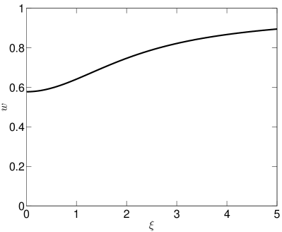
Figure 1.— Signal propagation speed $w$ of the telegraph equation for different values of $\xi$.

2.4. Anisotropy

The streaming anisotropy of the particle distribution is defined as

$$A(z,t)=\frac{3\int_{-1}^{1}\mu f\mathrm{d}\mu}{\int_{-1}^{1}f\mathrm{d}\mu}=\frac{3S}{vF_{0}},$$ (22)

where $S$ is the accordingly defined particle flux. Litvinenko & Schlickeiser (2013) calculated the streaming anisotropy in the telegraph approximation (their Eq. 32 in a slightly different notation):

$$A(z,t)=\frac{1}{F_{0}}\left(\tau\frac{\partial^{2}F_{0}}{\partial t\partial z}-\frac{\partial F_{0}}{\partial z}\right).$$ (23)

In terms of the linear density, the anisotropy is expressed as follows:

$$A(z,t)=\frac{1}{F}\left(\tau\frac{\partial^{2}F}{\partial t\partial z}-\frac{\partial F}{\partial z}\right)+\xi\left(1-\frac{\tau}{F}\frac{\partial F}{\partial t}\right).$$ (24)

In the diffusion approximation, the anisotropy is obtained by formally setting $\tau=0$:

$$A(z,t)=-\frac{1}{F_{0}}\frac{\partial F_{0}}{\partial z},$$ (25)

which, upon inserting the fundamental solution from Eq. (7) gives

$$A(z,t)=\frac{\xi}{2}+\frac{z}{2\kappa_{\parallel}t}.$$ (26)

3. Stochastic simulation scheme

Stochastic differential equations are used in many contexts to solve Fokker-Planck type equations. In space physics, they are often employed to solve particle propagation problems, such as cosmic-ray modulation (Strauss et al., 2011; Effenberger et al., 2012), SEP transport (Dröge et al., 2010), shock acceleration (Achterberg & Schure, 2011; Zuo et al., 2011), and pick-up ion evolution (Fichtner et al., 1996; Chalov & Fahr, 1998). For a recent account of numerical methods and issues connected to this approach, see, e.g., Kopp et al. (2012).

The application of the Ito calculus gives a system of stochastic differential equations, which is completely equivalent to the Fokker-Planck equation for the linear density, namely (Gardiner, 2009)

$$dz =\mu vdt,$$ (27)

$$d\mu =\left[\frac{v}{2L}(1-\mu^{2})-2D_{0}\mu\right]dt+\sqrt{2D_{0}(1-\mu^{2})}dW,$$ (28)

where $W(t)$ represents a Wiener process with zero mean and variance $t$.

We nondimensionalize this system of equations and solve it numerically, using the Milstein approximation scheme (Litvinenko & Noble, 2013; Kloeden & Platen, 1995):

$$z_{t+\Delta t} =z_{t}+\mu_{t}\Delta t,$$ (29)

$$\mu_{t+\Delta t} =\left[\frac{1}{2}\xi(1-\mu_{t}^{2})-\mu_{t}\right]\Delta t+\sqrt{\Delta t(1-\mu_{t}^{2})}\epsilon_{t}$$

$$-\frac{1}{2}\mu_{t}\Delta t(\epsilon_{t}^{2}-1),$$ (30)

where $\epsilon_{t}$ is a normal random variable with zero mean and unity variance. We use reflecting boundaries at $\mu=\pm 1$ to conserve the probability. The following comparisons with the approximate analytical solutions are performed by simulating a large number of pseudo-particle orbits according to the above scheme and obtaining the distribution functions by corresponding averages over the particle positions.

We used an isotropic initial pitch-angle distribution in our simulations. Although the SEP injection can be non-isotropic, the influence of the initial condition is insignificant after a brief transitional period of a few scattering times (see a recent discussion in Litvinenko & Noble, 2013, and in particular their Figures 3 and 4). We verified independently that the results presented in the following section are only slightly altered if the initial pitch-angle distribution is proportional to a delta function.

4. Results

4.1. Spatial intensity behavior

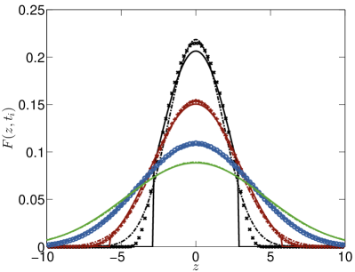
Figure 2.— Isotropic linear density $F(z,t_{i})$ at four different times, namely $t_{1}=5$ (black, ’x’), $t_{2}=10$ (red, ’+’), $t_{3}=20$ (blue, ’o’) and $t_{4}=30$ (green, ’.’) in the case of no focusing ($\xi=0$). The solid lines show the solution of the telegraph equation, given by Eq. (18). The dot-dashed lines give the solution of the diffusion approximation (Eq. 7). The symbols show the numerical results, obtained by iterating Eqs. (29) and (30), i.e. the full focused transport problem, with $10^{7}$ particles starting at the origin in each run, and averaging without regard to the pitch-angle of the particles.

To assess the range of validity of the telegraph equation, we performed stochastic simulations of the type described in the preceding section with $10^{7}$ particles starting at the origin in each run. We then binned the particles in intervals of length 0.1 and normalized with respect to the number of particles to get a spatial profile of the particle distribution function (linear density). We compared the results with the analytical solution of the telegraph equation, given by Eqs. (20) and (18), evaluated for different times $t_{i}$. Fig. 2 shows the results at four different times in the case of no focusing ($\xi=0$). A good agreement between the telegraph solution and the stochastic simulation is found, especially at later times. For comparison we also show the solution in the diffusion approximation (Eq. 7), which is equally good in this case (see also Kota et al., 1982). Note, however, a slight overshoot of the diffusion solution at the early time ($t_{1}=5$), indicating the non-causality. At $t=t_{1}=5$, no particle could have traveled farther from the origin than $z=vt_{1}=5$. The telegraph solution, on the other hand, somewhat underestimates the intensity at larger distances at early times, due to its lower signal propagation speed $w<v$ (Fig. 1).

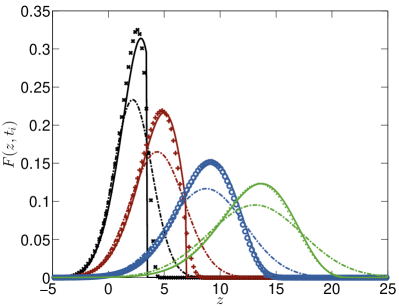
Figure 3.— Similar to Fig. 2 but for the case of strong focusing ($\xi=1.5$).

Fig. 3 gives similar plots for the case of strong focusing ($\xi=1.5$). Here, large differences between the telegraph and the diffusion solution become visible, reinforcing the results in Litvinenko & Noble (2013). Clearly in this case the telegraph approximation reproduces an evolving density pulse much better than the diffusion approximation for all times. A feature of interest is an asymmetry of the density profile due to the finite particle speed: a sharp front, followed by an extended wake.

4.2. Temporal intensity behavior

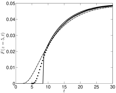
Figure 4.— Time profile of the isotropic linear density $F$ at a fixed position $z=5$ in the case of no focusing ($\xi=0$). The solid line is the analytical solution of the telegraph equation. The dot-dashed line gives the solution in the diffusion approximation. The symbols are produced from the same simulations as in Fig. 2.

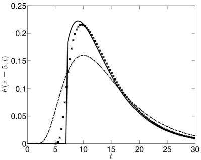
Figure 5.— Similar to Fig. 4 but for the case of strong focusing ($\xi=1.5$).

Time profiles of particle intensities are an important tool for analyzing the SEP data. Therefore, we extended our comparison to time profiles at a fixed position. Motivated by the data analysis in Artmann et al. (2011), we chose $z=5$ and, as previously, investigated two cases, namely those of no focusing ($\xi=0$) in Fig. 4 and strong focusing ($\xi=1.5$) in Fig. 5. While the diffusion approximation and the telegraph equation are equally valid in the non-focusing limit for $t>z/w$, both approximations break down at earlier times. By contrast, Fig. 5 shows that the telegraph equation is much more accurate than the diffusion approximation in the strong focusing case. Only at very late times, both approximations predict the same value of the intensity.

4.3. Temporal anisotropy behavior

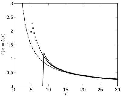
Figure 6.— Time profile of the anisotropy $A$ at the fixed position $z=5$ in the case of no focusing ($\xi=0$). The solid line is the numerical solution of Eq. (24). The dot-dashed line gives the solution in the diffusion approximation (Eq. 26). The symbols show the numerical result for the anisotropy, evaluated from the distribution of $10^{7}$ particles, according to Eq. (22).

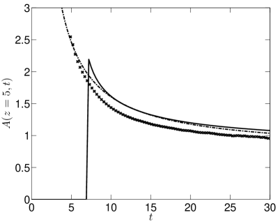
Figure 7.— Similar to Fig. 6 but for the case of strong focusing ($\xi=1.5$).

Additional information about energetic particle transport can be obtained by analyzing the streaming anisotropy $A(z,t)$ of the observed SEP data. We used the stochastic simulation results to compute the anisotropy, defined by Eq. (22), and we compared it with the predictions of the diffusion and telegraph approximations. We evaluated equation (24) numerically (with a simple finite-difference method), since the analytical expressions become quite cumbersome and give no further insight.

Figs. 6 and 7 show the resulting anisotropy profiles at $z=5$ for two cases: no focusing ($\xi=0$) and strong focusing ($\xi=1.5$), respectively. Somewhat surprisingly, it appears that the accuracy of either approximation is almost the same, with both predictions slightly overestimating $A$ in comparison with the numerical results for the case of strong focusing, even for $t\gg 1$. The telegraph approximation, however, captures the early time behavior better for vanishing focusing, although it cannot accurately model the anisotropy at even earlier times $t<z/w$. The diffusion approximation can at least give a rough estimate in the interval $z/v<t<z/w$. Thus the telegraph equation, in our parameter range, yields only a slightly better estimate for $A$ in comparison with the diffusion approximation and only in a situation of weak or absent focusing.

5. Discussion

The telegraph equation approximates a general transport equation in a number of transport problems, and so it is often desirable to know how accurate the telegraph approximation is, especially in comparison with the simpler diffusion approximation (Gombosi et al., 1993; Porra et al., 1997). In this paper we investigated the validity of the telegraph approximation in a model problem of solar energetic particle transport in interplanetary space. We extended recent studies (Litvinenko & Noble, 2013; Litvinenko & Schlickeiser, 2013) by analytically solving an initial value problem for the telegraph equation, calculating the SEP intensity profiles in space and time, and comparing the profiles with those obtained from a stochastic numerical solution of the Fokker-Planck equation.

We conclude that the telegraph approximation reproduces the SEP intensity profile much more accurately than the diffusion approximation. The result appears to be related to the finite signal propagation speed in the telegraph equation, which implies that the telegraph approximation can describe both diffusive and wavelike aspects of the intensity evolution. Somewhat surprisingly, we found that the telegraph approximation offers no significant advantage over the diffusion approximation for calculating the anisotropy of the SEP distribution function, with both approximations overestimating the anisotropy for strong focusing. Consequently, the full Fokker-Planck equation should be solved in order to determine the pitch-angle distribution of the energetic particles.

The key simplifying assumptions of the model in this paper are the isotropic pitch-angle scattering rate $D_{\mu\mu}$ and a constant adiabatic focusing length $L$ of a guiding magnetic field. Although $L=\mbox{const}$ is often assumed in theoretical studies (Earl, 1976; Litvinenko & Schlickeiser, 2011), the assumption is valid only as long as the focusing length $L$ does not change appreciably over one scattering length $\simeq v/D_{0}$. As we discuss in the Appendix, however, the condition is unlikely to be satisfied for the SEP transport close to the Sun.

In the future we plan to relax both assumptions by deriving a more general telegraph-type equation and by stochastically simulating the Fokker-Planck equation with more realistic $D_{\mu\mu}$ and $L=L(z)$. (Note that Earl (1981) developed a diffusion approximation with $L=L(z)$.) Further improvements could include more realistic boundary conditions, say a reflecting inner boundary. Recent studies also emphasized the potential role of the observed strong perpendicular transport (Dresing et al., 2012; Laitinen et al., 2013; Dröge et al., 2010), drifts (Marsh et al., 2013), and modeling of pitch-angle diffusion with full-orbit methods (e.g., Tautz et al., 2013; Tautz, 2013; Laitinen et al., 2012; Tautz et al., 2012).

To sum up, we presented a systematic side-by-side comparison of the predictions for the SEP transport, made using the diffusion and telegraph approximations and the Fokker-Planck equation on which the approximations are based. We deliberately adopted the simplest physically meaningful model: isotropic scattering, a constant focusing length, no advection, momentum diffusion or adiabatic deceleration. The essential point is that, while various features of the SEP transport had been previously investigated in detail numerically (e.g., Zank et al., 2000; Lu et al., 2001; Kaghashvili et al., 2004), we believe that a simple analytical model for the key features of the particle transport is valuable since it can guide the numerical studies. In the future we intend to relax the simplifying assumptions of this paper in order to explore the usefulness of the telegraph approximation more fully.

Appendix A The focusing length between the Sun and 1 AU

We discuss the radial dependence of the focusing length in the Parker interplanetary magnetic field, to quantify the accuracy of the assumption of constant focusing for SEPs. The Parker magnetic field in spherical coordinates ($r,\vartheta,\varphi$) is given by (Parker, 1958)

$$B_{r} =B_{0}(r_{0})\left(\frac{r_{0}}{r}\right)^{2},$$ (A1)

$$B_{\vartheta} =0,$$ (A2)

$$B_{\varphi} =-B_{r}\frac{r\Omega}{u_{sw}}\sin\vartheta.$$ (A3)

We assume a constant solar wind speed of $u_{sw}=400$ km/s and a constant angular velocity of the Sun of $\Omega=2\pi/25$d. In the following, we consider the case $\vartheta=\pi/2$, i.e. the field in the ecliptic plane.

The total magnetic field strength is given by

$$B=\frac{B(r_{0})}{r^{2}}\sqrt{1+(\beta r)^{2}},$$ (A4)

where we have introduced $\beta=-\Omega/u_{sw}$, which has a value of $\beta=-1.09$ AU^-1 for our choice of parameters.

The focusing length $L$ in the Parker spiral field is given by

$$\frac{1}{L} =-\frac{1}{B}\frac{\partial B}{\partial r}\frac{\mathrm{d}r}{\mathrm{d}z}$$

$$=\left(-\frac{1}{B}\right)\cdot\left(-B\frac{2+(\beta r)^{2}}{r(1+(\beta r)^{2}}\right)\cdot\frac{1}{\sqrt{(1+(\beta r)^{2}}},$$ (A5)

and so

$$L(r)=\frac{r(1+(\beta r)^{2})^{3/2}}{2+(\beta r)^{2}}.$$ (A6)

More details on the derivation of characteristic parameters in the Parker field can be found, e.g., in Artmann (2013).

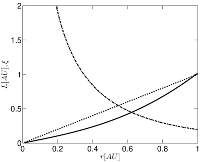
Figure 8.— Spatial behavior of the focusing length $L$ (solid) and the focusing parameter $\xi$ (dot-dashed) in the Parker magnetic field between the Sun and 1 AU, assuming a constant mean free path of $0.2$ AU. The straight radial line (dotted) is included to guide the eye.

Fig. (8) shows the spatial dependence of the focusing length and the dimensionless focusing parameter $\xi=\lambda_{0}/L$ between the Sun and 1 AU. We assumed a typical value for the constant mean free path $\lambda_{0}$ of 0.2 AU. The focusing length varies strongly, and consequently $\xi$ can have both very large and very small values (depending on the mean free path) between the Sun and 1 AU.

References

- Achterberg & Schure (2011) Achterberg, A., & Schure, K. M. 2011, MNRAS, 411, 2628
- Artmann (2013) Artmann, S. 2013, PhD thesis, Ruhr-University Bochum, Germany
- Artmann et al. (2011) Artmann, S., Schlickeiser, R., Agueda, N., Krucker, S., & Lin, R. P. 2011, A&A, 535, A92
- Beeck & Wibberenz (1986) Beeck, J., & Wibberenz, G. 1986, ApJ, 311, 437
- Chalov & Fahr (1998) Chalov, S. V., & Fahr, H. J. 1998, A&A, 335, 746
- Dresing et al. (2012) Dresing, N., Gómez-Herrero, R., Klassen, A., Heber, B., Kartavykh, Y., & Dröge, W. 2012, Sol. Phys., 281, 281
- Dröge et al. (2010) Dröge, W., Kartavykh, Y. Y., Klecker, B., & Kovaltsov, G. A. 2010, ApJ, 709, 912
- Earl (1974) Earl, J. A. 1974, ApJ, 193, 231
- Earl (1976) —. 1976, ApJ, 205, 900
- Earl (1981) —. 1981, ApJ, 251, 739
- Effenberger et al. (2012) Effenberger, F., Fichtner, H., Scherer, K., Barra, S., Kleimann, J., & Strauss, R. D. 2012, ApJ, 750, 108
- Fichtner et al. (1996) Fichtner, H., Le Roux, J. A., Mall, U., & Rucinski, D. 1996, A&A, 314, 650
- Fisk & Axford (1969) Fisk, L. A., & Axford, W. I. 1969, Sol. Phys., 7, 486
- Gardiner (2009) Gardiner, C. W. 2009, Stochastic Methods: A Handbook for the Natural and Social Sciences (Berlin: Springer)
- Gombosi et al. (1993) Gombosi, T. I., Jokipii, J. R., Kota, J., Lorencz, K., & Williams, L. L. 1993, ApJ, 403, 377
- Hasselmann & Wibberenz (1970) Hasselmann, K., & Wibberenz, G. 1970, ApJ, 162, 1049
- Jokipii (1966) Jokipii, J. R. 1966, ApJ, 146, 480
- Kaghashvili et al. (2004) Kaghashvili, E. K., Zank, G. P., Lu, J. Y., & Dröge, W. 2004, Journal of Plasma Physics, 70, 505
- Kloeden & Platen (1995) Kloeden, P., & Platen, E. 1995, Numerical methods for stochastic differential equations (Spinger, Berlin)
- Kopp et al. (2012) Kopp, A., Büsching, I., Strauss, R. D., & Potgieter, M. S. 2012, Computer Physics Communications, 183, 530
- Kota et al. (1982) Kota, J., Merenyi, E., Jokipii, J. R., Kopriva, D. A., Gombosi, T. I., & Owens, A. J. 1982, ApJ, 254, 398
- Laitinen et al. (2012) Laitinen, T., Dalla, S., & Kelly, J. 2012, ApJ, 749, 103
- Laitinen et al. (2013) Laitinen, T., Dalla, S., & Marsh, M. S. 2013, ApJ, 773, L29
- Litvinenko & Noble (2013) Litvinenko, Y. E., & Noble, P. L. 2013, ApJ, 765, 31
- Litvinenko & Schlickeiser (2011) Litvinenko, Y. E., & Schlickeiser, R. 2011, ApJ, 732, L31
- Litvinenko & Schlickeiser (2013) —. 2013, A&A, 554, A59
- Lu et al. (2001) Lu, J. Y., Zank, G. P., & Webb, G. M. 2001, ApJ, 550, 34
- Marsh et al. (2013) Marsh, M. S., Dalla, S., Kelly, J., & Laitinen, T. 2013, ApJ, 774, 4
- Parker (1958) Parker, E. N. 1958, ApJ, 128, 664
- Pauls & Burger (1994) Pauls, H. L., & Burger, R. A. 1994, ApJ, 427, 927
- Porra et al. (1997) Porra, J. M., Masoliver, J., & Weiss, G. H. 1997, Phys. Rev. E, 55, 7771
- Roelof (1969) Roelof, E. C. 1969, in Lectures in High-Energy Astrophysics, ed. H. Ögelman & J. R. Wayland, 111
- Schlickeiser (2011) Schlickeiser, R. 2011, ApJ, 732, 96
- Schlickeiser & Shalchi (2008) Schlickeiser, R., & Shalchi, A. 2008, ApJ, 686, 292
- Schwadron & Gombosi (1994) Schwadron, N. A., & Gombosi, T. I. 1994, J. Geophys. Res., 99, 19301
- Shalchi et al. (2009) Shalchi, A., Koda, T. Å., Tautz, R. C., & Schlickeiser, R. 2009, A&A, 507, 589
- Shea & Smart (2012) Shea, M. A., & Smart, D. F. 2012, Space Sci. Rev., 171, 161
- Strauss et al. (2011) Strauss, R. D., Potgieter, M. S., Büsching, I., & Kopp, A. 2011, ApJ, 735, 83
- Tautz (2013) Tautz, R. C. 2013, A&A, 558, A148
- Tautz et al. (2013) Tautz, R. C., Dosch, A., Effenberger, F., Fichtner, H., & Kopp, A. 2013, A&A, 558, A147
- Tautz et al. (2012) Tautz, R. C., Dosch, A., & Lerche, I. 2012, A&A, 545, A149
- Zank et al. (2000) Zank, G. P., Lu, J. Y., Rice, W. K. M., & Webb, G. M. 2000, Journal of Plasma Physics, 64, 507
- Zuo et al. (2011) Zuo, P., Zhang, M., Gamayunov, K., Rassoul, H., & Luo, X. 2011, ApJ, 738, 168