Correcting the spectroscopic surface gravity using transits and asteroseismology

Abstract

Context. Precise stellar parameters (effective temperature, surface gravity, metallicity, stellar mass, and radius) are crucial for several reasons, amongst which are the precise characterization of orbiting exoplanets and the correct determination of galactic chemical evolution. The atmospheric parameters are extremely important because all the other stellar parameters depend on them. Using our standard equivalent-width method on high-resolution spectroscopy, good precision can be obtained for the derived effective temperature and metallicity. The surface gravity, however, is usually not well constrained with spectroscopy.

Aims. We use two different samples of FGK dwarfs to study the effect of the stellar surface gravity on the precise spectroscopic determination of the other atmospheric parameters. Furthermore, we present a straightforward formula for correcting the spectroscopic surface gravities derived by our method and with our linelists.

Methods. Our spectroscopic analysis is based on Kurucz models in LTE, performed with the MOOG code to derive the atmospheric parameters. The surface gravity was either left free or fixed to a predetermined value. The latter is either obtained through a photometric transit light curve or derived using asteroseismology.

Results. We find first that, despite some minor trends, the effective temperatures and metallicities for FGK dwarfs derived with the described method and linelists are, in most cases, only affected within the errorbars by using different values for the surface gravity, even for very large differences in surface gravity, so they can be trusted. The temperatures derived with a fixed surface gravity continue to be compatible within 1 sigma with the accurate results of the InfraRed Flux Method (IRFM), as is the case for the unconstrained temperatures. Secondly, we find that the spectroscopic surface gravity can easily be corrected to a more accurate value using a linear function with the effective temperature.

1 Introduction

Precise stellar parameters, such as effective temperature, surface gravity, metallicity, stellar mass, and stellar radius, are crucial for several reasons in astronomy. Amongst these, there are the precise characterization of planetary systems (e.g. Torres et al., 2012; Mortier et al., 2013c), discovery of the possible link between the properties of stars and the existence of a planet (e.g. Adibekyan et al., 2013b; Beaugé & Nesvorný, 2013; Mortier et al., 2013a), and the complete and accurate picture of Galactic evolution (e.g. Edvardsson et al., 1993; McWilliam et al., 2008; Minchev et al., 2013).

In the ever-growing exoplanetary field, accurate and precise stellar parameters are necessary for the precise characterization of exoplanets. The main bulk of the discovered exoplanets has been found using radial velocities and/or the photometric transit technique. Separately, these techniques only partly characterize the planet. With radial velocities, a constraint is put on the planetary mass ($M_{p}\sin i$), while the transit technique is used to determine the planetary radius ($R_{p}$). Good knowledge of both these properties is essential for understanding the different kinds of planets and their distributions in the Galaxy (e.g. Buchhave et al., 2014; Dumusque et al., 2014; Marcy et al., 2014).

However, these planetary characteristics (mass, radius, and thus mean density) are highly dependent on the knowledge of the stellar characteristics ($M_{p}\propto M_{\ast}^{2/3}$ and $R_{p}\propto R_{\ast}$) (e.g. Torres et al., 2012; Mortier et al., 2013c). The stellar mass and radius, in turn, depend on the effective temperature, surface gravity, and the metallicity of the star, therefore it is extremely important to obtain precise atmospheric stellar properties.

Furthermore, to minimize the errors and to obtain comparable results, a uniform analysis is required (Torres et al., 2008, 2012; Santos et al., 2013) to guarantee the best possible homogeneity in the results. By homogeneously deriving precise stellar parameters we also gain more than just improving planetary parameters. Observational and theoretical works have shown that the processes of planet formation and evolution seem to depend on several stellar properties, such as stellar metallicity and mass (e.g. Butler et al., 2006; Udry & Santos, 2007; Bowler et al., 2010; Johnson et al., 2010; Mayor et al., 2011; Sousa et al., 2011; Mordasini et al., 2012; Mortier et al., 2013a; Adibekyan et al., 2013b). With large samples of planet hosts with homogeneously derived stellar and planetary parameters, we can look for correlations between the various parameters and statistically evaluate them. These correlations will allow us to narrow down the theories of planet formation.

Not just exoplanetary science benefits from having precise, accurate, and homogeneous stellar properties. These can also be useful to explain the formation and evolution of stars and thus of our Galaxy, which consists of different structures all with different properties. It has been shown for example that there is a difference in metallicity (iron and other heavy elements) between the thin disk and the thick disk (e.g. Edvardsson et al., 1993; Bensby et al., 2005; Haywood, 2008; Adibekyan et al., 2013a). To properly understand the different stellar populations and their origins in the Milky Way, we need precise and homogeneous stellar parameters.

To derive a set of precise stellar properties (effective temperature $T_{\mathrm{eff}}$, surface gravity $\log g$, metallicity [Fe/H], and microturbulence $\xi$), high-resolution spectroscopy is usually the best approach. Commonly, two methods are used to analyse these spectra: spectral synthesis and spectral line analysis. The first method compares observed spectra with synthetic ones, for example with the code SME (Valenti & Piskunov, 1996) or MATISSE (Recio-Blanco et al., 2006). Spectral line analysis, as used in this work, makes use of the equivalent width (EW) of absorption lines (usually the Fe i and Fe ii lines) to demand excitation and ionization equilibrium.

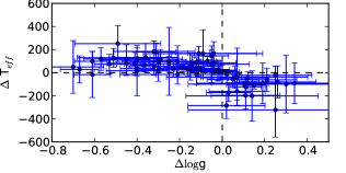
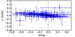
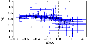
Figure 1: Differences of the spectroscopic results (left to right: effective temperature, metallicity, and microturbulence) as a function of the difference in $\log$g (defined as ‘constrained with transit $\log g$ - unconstrained’).

Both methods have been shown to provide surface gravities that are not well constrained and do not compare well with surface gravities as obtained from other non-spectroscopic methods, such as asteroseismology or stellar models (e.g. Torres et al., 2012; Huber et al., 2013; Mortier et al., 2013c). This surface gravity is important for the determination of the stellar mass and especially the stellar radius as shown in Mortier et al. (2013c).

In this work, we take a closer look at the surface gravity and its effect on the determination of the other atmospheric parameters. In Section 2, we present the uniform spectroscopic method we use. Section 3 handles the effect of fixing the surface gravity to a value obtained by transit photometry and a possible correction formula. The same study is then done for the more accurate surface gravities as obtained by asteroseismolgy (Section 4). Finally, we discuss in Section 5.

2 Spectroscopic method

Over the years, we have developed a homogeneous method to derive stellar parameters (e.g. Santos et al., 2004; Sousa et al., 2008, 2011; Tsantaki et al., 2013). This method is based on the analysis of iron lines from high-resolution spectra. Details of this method can be found in Santos et al. (2013) and references therein. Here we only give an overview of the method.

EWs of iron lines (Fe I and Fe II) are automatically calculated with the code ARES (Automatic Routine for line Equivalent widths in stellar Spectra - Sousa et al., 2007) for which the large lists with stable lines of Sousa et al. (2008) and Tsantaki et al. (2013) are used for stars hotter and cooler than 5200 K, respectively. These EWs are then used together with a grid of ATLAS plane-parallel model atmospheres (Kurucz, 1993) to determine the atmospheric stellar parameters, $T_{\mathrm{eff}}$, $\log g$, [Fe/H], and $\xi$. Therefore, we use the MOOG code (Sneden, 1973) in which we assume Local Thermodynamic Equilibrium (LTE).

By imposing excitation and ionization equilibrium, the atmospheric parameters are determined using an iterative minimization code based on the Downhill Simplex Method (Press et al., 1992).

The same method can be used whilst fixing the surface gravity to a predetermined value (see next Sections). In this case however, ionization equilibrium will not be imposed as this is the main condition for determining the surface gravity. As a direct result, we do not use the Fe II lines anymore. The value for the metallicity is thus determined by only using the Fe I lines.

longtablecccccccc Stellar (unconstrained) spectroscopic parameters used in this work. The last two columns contain the surface gravities as calculated with Equation 3, resp. Equation 4
Name T_eff,spec $\log g_{spec}$ [Fe/H]_spec $\xi_{spec}$ Ref. $\log g_{corr,1}$ $\log g_{corr,2}$
(K) (dex) (dex) (km s^-1) (dex) (dex)
continued.
Name T_eff,spec $\log g_{spec}$ [Fe/H]_spec $\xi_{spec}$ Ref. $\log g_{corr,1}$ $\log g_{corr,2}$
(K) (dex) (dex) (km s^-1) (dex) (dex)
CoRoT-1 6397 $\pm$ 54 4.66 $\pm$ 0.09 0.03 $\pm$ 0.04 1.68 $\pm$ 0.09 (1) 4.32 $\pm$ 0.24 4.27 $\pm$ 0.22
CoRoT-10 5025 $\pm$ 155 4.47 $\pm$ 0.31 0.06 $\pm$ 0.09 1.26 $\pm$ 0.34 (1) 4.76 $\pm$ 0.37 4.62 $\pm$ 0.36
CoRoT-12 5715 $\pm$ 208 4.66 $\pm$ 0.22 0.17 $\pm$ 0.14 1.07 $\pm$ 0.31 (1) 4.63 $\pm$ 0.32 4.54 $\pm$ 0.30
CoRoT-2 5697 $\pm$ 97 4.73 $\pm$ 0.17 -0.09 $\pm$ 0.07 1.64 $\pm$ 0.16 (1) 4.71 $\pm$ 0.27 4.61 $\pm$ 0.26
CoRoT-4 6344 $\pm$ 93 4.82 $\pm$ 0.11 0.15 $\pm$ 0.06 1.74 $\pm$ 0.14 (1) 4.50 $\pm$ 0.25 4.45 $\pm$ 0.23
CoRoT-5 6240 $\pm$ 70 4.46 $\pm$ 0.11 0.04 $\pm$ 0.05 1.28 $\pm$ 0.09 (1) 4.19 $\pm$ 0.25 4.13 $\pm$ 0.23
CoRoT-7 5288 $\pm$ 27 4.40 $\pm$ 0.07 0.02 $\pm$ 0.02 0.90 $\pm$ 0.05 (1) 4.57 $\pm$ 0.21 4.44 $\pm$ 0.20
CoRoT-8 5143 $\pm$ 178 4.42 $\pm$ 0.33 0.22 $\pm$ 0.11 0.61 $\pm$ 0.40 (1) 4.65 $\pm$ 0.39 4.52 $\pm$ 0.38
CoRoT-9 5613 $\pm$ 36 4.35 $\pm$ 0.09 -0.02 $\pm$ 0.03 0.90 $\pm$ 0.05 (1) 4.37 $\pm$ 0.23 4.27 $\pm$ 0.21
HAT-P-1 6076 $\pm$ 27 4.47 $\pm$ 0.07 0.21 $\pm$ 0.03 1.17 $\pm$ 0.05 (1) 4.28 $\pm$ 0.23 4.21 $\pm$ 0.21
HAT-P-11 4624 $\pm$ 225 4.15 $\pm$ 0.59 0.26 $\pm$ 0.08 0.39 $\pm$ 0.70 (1) 4.62 $\pm$ 0.63 4.45 $\pm$ 0.62
HAT-P-17 5332 $\pm$ 55 4.45 $\pm$ 0.13 0.05 $\pm$ 0.03 0.82 $\pm$ 0.10 (1) 4.60 $\pm$ 0.24 4.48 $\pm$ 0.23
HAT-P-20 4502 $\pm$ 188 4.32 $\pm$ 0.60 0.12 $\pm$ 0.15 0.73 $\pm$ 0.60 (1) 4.85 $\pm$ 0.64 4.67 $\pm$ 0.63
HAT-P-26 5011 $\pm$ 55 4.31 $\pm$ 0.17 0.01 $\pm$ 0.04 0.48 $\pm$ 0.16 (1) 4.60 $\pm$ 0.26 4.46 $\pm$ 0.25
HAT-P-27 5316 $\pm$ 55 4.48 $\pm$ 0.10 0.30 $\pm$ 0.03 0.82 $\pm$ 0.09 (1) 4.63 $\pm$ 0.23 4.51 $\pm$ 0.21
HAT-P-30 6338 $\pm$ 42 4.52 $\pm$ 0.06 0.12 $\pm$ 0.03 1.40 $\pm$ 0.05 (1) 4.21 $\pm$ 0.23 4.16 $\pm$ 0.21
HAT-P-35 6178 $\pm$ 45 4.40 $\pm$ 0.09 0.12 $\pm$ 0.03 1.34 $\pm$ 0.06 (1) 4.16 $\pm$ 0.24 4.10 $\pm$ 0.22
HAT-P-4 6054 $\pm$ 60 4.17 $\pm$ 0.28 0.35 $\pm$ 0.08 1.59 $\pm$ 0.09 (1) 3.99 $\pm$ 0.35 3.92 $\pm$ 0.34
HAT-P-6 6855 $\pm$ 111 4.69 $\pm$ 0.20 -0.08 $\pm$ 0.11 2.85 $\pm$ 1.15 (1) 4.14 $\pm$ 0.31 4.12 $\pm$ 0.29
HAT-P-7 6525 $\pm$ 61 4.09 $\pm$ 0.08 0.31 $\pm$ 0.07 1.78 $\pm$ 0.14 (1) 3.69 $\pm$ 0.24 3.65 $\pm$ 0.22
HAT-P-8 6550 $\pm$ 61 4.80 $\pm$ 0.08 0.07 $\pm$ 0.04 1.93 $\pm$ 0.09 (1) 4.39 $\pm$ 0.24 4.35 $\pm$ 0.22
HD149026 6162 $\pm$ 41 4.37 $\pm$ 0.10 0.36 $\pm$ 0.05 1.41 $\pm$ 0.07 (1) 4.14 $\pm$ 0.24 4.07 $\pm$ 0.22
HD17156 6084 $\pm$ 29 4.33 $\pm$ 0.05 0.23 $\pm$ 0.04 1.47 $\pm$ 0.05 (1) 4.13 $\pm$ 0.22 4.06 $\pm$ 0.21
HD189733 5109 $\pm$ 146 4.69 $\pm$ 0.28 0.03 $\pm$ 0.08 0.78 $\pm$ 0.33 (1) 4.94 $\pm$ 0.35 4.80 $\pm$ 0.34
HD209458 6118 $\pm$ 25 4.50 $\pm$ 0.04 0.03 $\pm$ 0.02 1.21 $\pm$ 0.03 (1) 4.29 $\pm$ 0.22 4.22 $\pm$ 0.20
HD80606 5574 $\pm$ 72 4.46 $\pm$ 0.20 0.32 $\pm$ 0.09 1.14 $\pm$ 0.09 (1) 4.50 $\pm$ 0.29 4.39 $\pm$ 0.28
HD97658 5137 $\pm$ 36 4.47 $\pm$ 0.09 -0.35 $\pm$ 0.02 0.63 $\pm$ 0.08 (1) 4.71 $\pm$ 0.22 4.57 $\pm$ 0.21
Kepler-17 5781 $\pm$ 85 4.53 $\pm$ 0.12 0.26 $\pm$ 0.10 1.73 $\pm$ 0.14 (1) 4.47 $\pm$ 0.25 4.38 $\pm$ 0.23
Kepler-21 6409 $\pm$ 44 4.43 $\pm$ 0.06 -0.03 $\pm$ 0.03 1.86 $\pm$ 0.07 (1) 4.08 $\pm$ 0.23 4.04 $\pm$ 0.21
KOI-135 6041 $\pm$ 143 4.26 $\pm$ 0.05 0.33 $\pm$ 0.11 1.85 $\pm$ 0.26 (1) 4.08 $\pm$ 0.23 4.01 $\pm$ 0.21
KOI-204 5757 $\pm$ 134 4.15 $\pm$ 0.06 0.26 $\pm$ 0.10 1.75 $\pm$ 0.19 (1) 4.10 $\pm$ 0.23 4.01 $\pm$ 0.21
OGLE-TR-10 6075 $\pm$ 86 4.54 $\pm$ 0.15 0.28 $\pm$ 0.10 1.45 $\pm$ 0.14 (1) 4.35 $\pm$ 0.27 4.28 $\pm$ 0.25
OGLE-TR-111 4800 $\pm$ 177 4.24 $\pm$ 0.46 0.22 $\pm$ 0.15 0.30 $\pm$ 1.38 (1) 4.63 $\pm$ 0.51 4.47 $\pm$ 0.50
OGLE-TR-113 4781 $\pm$ 166 4.31 $\pm$ 0.41 0.03 $\pm$ 0.06 1.24 $\pm$ 0.29 (1) 4.71 $\pm$ 0.46 4.55 $\pm$ 0.45
OGLE-TR-132 6210 $\pm$ 59 4.51 $\pm$ 0.27 0.37 $\pm$ 0.07 1.23 $\pm$ 0.09 (1) 4.26 $\pm$ 0.35 4.20 $\pm$ 0.34
OGLE-TR-182 5924 $\pm$ 64 4.47 $\pm$ 0.18 0.37 $\pm$ 0.08 0.91 $\pm$ 0.09 (1) 4.35 $\pm$ 0.28 4.27 $\pm$ 0.27
OGLE-TR-211 6325 $\pm$ 91 4.22 $\pm$ 0.17 0.11 $\pm$ 0.10 1.63 $\pm$ 0.21 (1) 3.91 $\pm$ 0.28 3.86 $\pm$ 0.27
OGLE-TR-56 6119 $\pm$ 62 4.21 $\pm$ 0.19 0.25 $\pm$ 0.08 1.48 $\pm$ 0.11 (1) 4.00 $\pm$ 0.29 3.93 $\pm$ 0.28
TrES-1 5226 $\pm$ 38 4.40 $\pm$ 0.10 0.06 $\pm$ 0.05 0.90 $\pm$ 0.05 (1) 4.60 $\pm$ 0.22 4.47 $\pm$ 0.21
TrES-2 5795 $\pm$ 73 4.30 $\pm$ 0.13 0.06 $\pm$ 0.08 0.79 $\pm$ 0.12 (1) 4.24 $\pm$ 0.25 4.15 $\pm$ 0.24
TrES-3 5502 $\pm$ 157 4.44 $\pm$ 0.22 -0.10 $\pm$ 0.19 1.00 $\pm$ 0.30 (1) 4.51 $\pm$ 0.31 4.40 $\pm$ 0.30
TrES-4 6293 $\pm$ 96 4.20 $\pm$ 0.27 0.34 $\pm$ 0.10 2.01 $\pm$ 0.17 (1) 3.91 $\pm$ 0.35 3.85 $\pm$ 0.34
WASP-1 6252 $\pm$ 45 4.32 $\pm$ 0.05 0.23 $\pm$ 0.03 1.42 $\pm$ 0.05 (1) 4.05 $\pm$ 0.22 3.99 $\pm$ 0.21
WASP-10 4645 $\pm$ 125 4.27 $\pm$ 0.39 0.04 $\pm$ 0.05 0.58 $\pm$ 0.47 (1) 4.73 $\pm$ 0.44 4.56 $\pm$ 0.43
WASP-11 4881 $\pm$ 125 4.44 $\pm$ 0.31 0.01 $\pm$ 0.05 0.64 $\pm$ 0.24 (1) 4.79 $\pm$ 0.37 4.64 $\pm$ 0.36
WASP-12 6313 $\pm$ 52 4.37 $\pm$ 0.12 0.21 $\pm$ 0.04 1.65 $\pm$ 0.07 (1) 4.07 $\pm$ 0.25 4.02 $\pm$ 0.24
WASP-13 6025 $\pm$ 21 4.19 $\pm$ 0.03 0.11 $\pm$ 0.05 1.28 $\pm$ 0.10 (1) 4.02 $\pm$ 0.22 3.95 $\pm$ 0.20
WASP-15 6573 $\pm$ 70 4.79 $\pm$ 0.08 0.09 $\pm$ 0.04 1.72 $\pm$ 0.09 (1) 4.37 $\pm$ 0.24 4.33 $\pm$ 0.22
WASP-16 5726 $\pm$ 22 4.34 $\pm$ 0.05 0.13 $\pm$ 0.02 0.97 $\pm$ 0.03 (1) 4.31 $\pm$ 0.22 4.21 $\pm$ 0.20
WASP-17 6794 $\pm$ 83 4.83 $\pm$ 0.09 -0.12 $\pm$ 0.05 2.57 $\pm$ 0.22 (1) 4.31 $\pm$ 0.25 4.29 $\pm$ 0.23
WASP-18 6526 $\pm$ 69 4.73 $\pm$ 0.08 0.19 $\pm$ 0.05 1.83 $\pm$ 0.10 (1) 4.33 $\pm$ 0.24 4.29 $\pm$ 0.22
WASP-19 5591 $\pm$ 62 4.46 $\pm$ 0.09 0.26 $\pm$ 0.05 1.23 $\pm$ 0.09 (1) 4.49 $\pm$ 0.23 4.39 $\pm$ 0.21
WASP-2 5109 $\pm$ 72 4.33 $\pm$ 0.14 0.02 $\pm$ 0.05 0.57 $\pm$ 0.12 (1) 4.58 $\pm$ 0.25 4.44 $\pm$ 0.23
WASP-21 5924 $\pm$ 55 4.39 $\pm$ 0.09 -0.22 $\pm$ 0.04 1.06 $\pm$ 0.08 (1) 4.27 $\pm$ 0.23 4.19 $\pm$ 0.22
WASP-22 6153 $\pm$ 46 4.57 $\pm$ 0.09 0.26 $\pm$ 0.03 1.36 $\pm$ 0.06 (1) 4.34 $\pm$ 0.24 4.28 $\pm$ 0.22
WASP-23 5046 $\pm$ 99 4.33 $\pm$ 0.18 0.05 $\pm$ 0.06 0.64 $\pm$ 0.23 (1) 4.61 $\pm$ 0.27 4.47 $\pm$ 0.26
WASP-24 6297 $\pm$ 58 4.76 $\pm$ 0.17 0.09 $\pm$ 0.04 1.41 $\pm$ 0.08 (1) 4.47 $\pm$ 0.28 4.41 $\pm$ 0.27
WASP-25 5736 $\pm$ 35 4.52 $\pm$ 0.09 0.06 $\pm$ 0.03 1.11 $\pm$ 0.05 (1) 4.48 $\pm$ 0.23 4.39 $\pm$ 0.21
WASP-26 6034 $\pm$ 31 4.44 $\pm$ 0.06 0.16 $\pm$ 0.02 1.28 $\pm$ 0.04 (1) 4.27 $\pm$ 0.22 4.19 $\pm$ 0.21
WASP-28 6134 $\pm$ 38 4.55 $\pm$ 0.05 -0.12 $\pm$ 0.03 1.17 $\pm$ 0.06 (1) 4.33 $\pm$ 0.22 4.26 $\pm$ 0.21
WASP-29 5203 $\pm$ 102 4.93 $\pm$ 0.21 0.17 $\pm$ 0.05 1.77 $\pm$ 0.22 (1) 5.14 $\pm$ 0.29 5.01 $\pm$ 0.28
WASP-31 6443 $\pm$ 75 4.76 $\pm$ 0.09 -0.08 $\pm$ 0.05 1.62 $\pm$ 0.11 (1) 4.40 $\pm$ 0.24 4.35 $\pm$ 0.23
WASP-32 6427 $\pm$ 141 4.93 $\pm$ 0.08 0.28 $\pm$ 0.10 1.20 $\pm$ 0.21 (1) 4.58 $\pm$ 0.24 4.53 $\pm$ 0.23
WASP-34 5704 $\pm$ 26 4.35 $\pm$ 0.05 0.08 $\pm$ 0.02 0.97 $\pm$ 0.03 (1) 4.33 $\pm$ 0.21 4.23 $\pm$ 0.20
WASP-35 6072 $\pm$ 62 4.69 $\pm$ 0.13 -0.05 $\pm$ 0.05 1.26 $\pm$ 0.09 (1) 4.50 $\pm$ 0.25 4.43 $\pm$ 0.24
WASP-36 5928 $\pm$ 59 4.51 $\pm$ 0.09 -0.01 $\pm$ 0.05 0.89 $\pm$ 0.09 (1) 4.38 $\pm$ 0.23 4.30 $\pm$ 0.22
WASP-38 6436 $\pm$ 60 4.80 $\pm$ 0.07 0.06 $\pm$ 0.04 1.75 $\pm$ 0.09 (1) 4.44 $\pm$ 0.23 4.40 $\pm$ 0.22
WASP-4 5513 $\pm$ 43 4.50 $\pm$ 0.07 0.03 $\pm$ 0.03 0.86 $\pm$ 0.07 (1) 4.56 $\pm$ 0.22 4.46 $\pm$ 0.20
WASP-41 5546 $\pm$ 33 4.53 $\pm$ 0.07 0.06 $\pm$ 0.02 1.08 $\pm$ 0.05 (1) 4.58 $\pm$ 0.22 4.47 $\pm$ 0.20
WASP-42 5315 $\pm$ 79 4.50 $\pm$ 0.18 0.29 $\pm$ 0.05 1.16 $\pm$ 0.13 (1) 4.65 $\pm$ 0.27 4.53 $\pm$ 0.26
WASP-47 5576 $\pm$ 68 4.28 $\pm$ 0.16 0.36 $\pm$ 0.05 1.25 $\pm$ 0.09 (1) 4.32 $\pm$ 0.26 4.21 $\pm$ 0.25
WASP-5 5785 $\pm$ 83 4.54 $\pm$ 0.14 0.17 $\pm$ 0.06 0.96 $\pm$ 0.12 (1) 4.48 $\pm$ 0.26 4.39 $\pm$ 0.24
WASP-50 5518 $\pm$ 42 4.43 $\pm$ 0.12 0.13 $\pm$ 0.03 1.25 $\pm$ 0.06 (1) 4.49 $\pm$ 0.24 4.38 $\pm$ 0.23
WASP-54 6296 $\pm$ 40 4.37 $\pm$ 0.06 0.00 $\pm$ 0.03 1.45 $\pm$ 0.05 (1) 4.08 $\pm$ 0.23 4.02 $\pm$ 0.21
WASP-55 6070 $\pm$ 53 4.55 $\pm$ 0.07 0.09 $\pm$ 0.04 1.10 $\pm$ 0.06 (1) 4.36 $\pm$ 0.23 4.29 $\pm$ 0.21
WASP-6 5383 $\pm$ 41 4.52 $\pm$ 0.06 -0.14 $\pm$ 0.03 0.80 $\pm$ 0.07 (1) 4.64 $\pm$ 0.21 4.53 $\pm$ 0.20
WASP-62 6391 $\pm$ 70 4.73 $\pm$ 0.11 0.24 $\pm$ 0.05 1.50 $\pm$ 0.09 (1) 4.39 $\pm$ 0.25 4.34 $\pm$ 0.23
WASP-63 5715 $\pm$ 60 4.29 $\pm$ 0.10 0.28 $\pm$ 0.05 1.28 $\pm$ 0.07 (1) 4.26 $\pm$ 0.23 4.17 $\pm$ 0.22
WASP-66 7051 $\pm$ 79 5.00 $\pm$ 0.08 0.05 $\pm$ 0.05 3.07 $\pm$ 0.27 (1) 4.36 $\pm$ 0.25 4.36 $\pm$ 0.23
WASP-67 5417 $\pm$ 85 4.40 $\pm$ 0.16 0.18 $\pm$ 0.06 1.16 $\pm$ 0.12 (1) 4.51 $\pm$ 0.26 4.39 $\pm$ 0.25
WASP-7 6621 $\pm$ 155 4.62 $\pm$ 0.14 0.12 $\pm$ 0.09 3.00 $\pm$ 0.83 (1) 4.18 $\pm$ 0.27 4.15 $\pm$ 0.26
WASP-71 6180 $\pm$ 52 4.15 $\pm$ 0.06 0.37 $\pm$ 0.04 1.69 $\pm$ 0.06 (1) 3.91 $\pm$ 0.23 3.85 $\pm$ 0.21
WASP-77A 5605 $\pm$ 41 4.37 $\pm$ 0.09 0.07 $\pm$ 0.03 1.09 $\pm$ 0.06 (1) 4.39 $\pm$ 0.23 4.29 $\pm$ 0.21
WASP-78 6291 $\pm$ 71 4.19 $\pm$ 0.08 -0.07 $\pm$ 0.05 1.63 $\pm$ 0.10 (1) 3.90 $\pm$ 0.24 3.84 $\pm$ 0.22
WASP-79 7002 $\pm$ 162 4.77 $\pm$ 0.14 0.19 $\pm$ 0.10 2.64 $\pm$ 0.24 (1) 4.15 $\pm$ 0.28 4.15 $\pm$ 0.26
WASP-8 5690 $\pm$ 36 4.42 $\pm$ 0.15 0.29 $\pm$ 0.03 1.25 $\pm$ 0.05 (1) 4.40 $\pm$ 0.26 4.31 $\pm$ 0.24
XO-1 5754 $\pm$ 42 4.61 $\pm$ 0.05 -0.01 $\pm$ 0.05 1.07 $\pm$ 0.09 (1) 4.56 $\pm$ 0.22 4.47 $\pm$ 0.20
KIC1430163 6833 $\pm$ 87 4.70 $\pm$ 0.11 0.02 $\pm$ 0.06 2.12 $\pm$ 0.10 (2) 4.16 $\pm$ 0.26 4.14 $\pm$ 0.24
KIC1435467 6485 $\pm$ 92 4.53 $\pm$ 0.13 0.08 $\pm$ 0.07 2.02 $\pm$ 0.09 (2) 4.15 $\pm$ 0.26 4.11 $\pm$ 0.25
KIC3427720 6111 $\pm$ 68 4.51 $\pm$ 0.11 0.04 $\pm$ 0.06 1.25 $\pm$ 0.04 (2) 4.30 $\pm$ 0.24 4.23 $\pm$ 0.23
KIC3456181 6584 $\pm$ 91 4.43 $\pm$ 0.11 -0.02 $\pm$ 0.07 2.01 $\pm$ 0.11 (2) 4.01 $\pm$ 0.25 3.97 $\pm$ 0.24
KIC3632418 6409 $\pm$ 74 4.43 $\pm$ 0.12 -0.03 $\pm$ 0.06 1.86 $\pm$ 0.06 (2) 4.09 $\pm$ 0.25 4.04 $\pm$ 0.24
KIC3643774 6125 $\pm$ 75 4.39 $\pm$ 0.12 0.25 $\pm$ 0.06 1.39 $\pm$ 0.05 (2) 4.18 $\pm$ 0.25 4.11 $\pm$ 0.23
KIC3656476 5719 $\pm$ 64 4.26 $\pm$ 0.11 0.28 $\pm$ 0.05 1.11 $\pm$ 0.03 (2) 4.23 $\pm$ 0.24 4.14 $\pm$ 0.22
KIC4072740 4960 $\pm$ 77 3.49 $\pm$ 0.13 0.19 $\pm$ 0.06 1.13 $\pm$ 0.06 (2) 3.81 $\pm$ 0.24 3.66 $\pm$ 0.23
KIC4346201 6239 $\pm$ 91 4.28 $\pm$ 0.12 -0.17 $\pm$ 0.07 1.64 $\pm$ 0.10 (2) 4.01 $\pm$ 0.25 3.95 $\pm$ 0.24
KIC4586099 6533 $\pm$ 80 4.37 $\pm$ 0.11 -0.04 $\pm$ 0.06 1.84 $\pm$ 0.08 (2) 3.97 $\pm$ 0.25 3.93 $\pm$ 0.24
KIC4638884 6684 $\pm$ 98 4.58 $\pm$ 0.17 -0.05 $\pm$ 0.08 3.39 $\pm$ 0.28 (2) 4.11 $\pm$ 0.29 4.08 $\pm$ 0.27
KIC4914923 5948 $\pm$ 65 4.34 $\pm$ 0.12 0.18 $\pm$ 0.05 1.26 $\pm$ 0.03 (2) 4.21 $\pm$ 0.25 4.13 $\pm$ 0.23
KIC4931390 6862 $\pm$ 80 4.55 $\pm$ 0.11 -0.02 $\pm$ 0.06 1.93 $\pm$ 0.09 (2) 4.00 $\pm$ 0.26 3.98 $\pm$ 0.24
KIC5184732_esp 5894 $\pm$ 68 4.31 $\pm$ 0.12 0.43 $\pm$ 0.06 1.18 $\pm$ 0.03 (2) 4.20 $\pm$ 0.25 4.12 $\pm$ 0.23
KIC5184732_nar 5877 $\pm$ 68 4.34 $\pm$ 0.11 0.40 $\pm$ 0.06 1.14 $\pm$ 0.03 (2) 4.24 $\pm$ 0.24 4.15 $\pm$ 0.23
KIC5371516 6526 $\pm$ 107 4.49 $\pm$ 0.15 0.11 $\pm$ 0.08 2.35 $\pm$ 0.14 (2) 4.09 $\pm$ 0.27 4.05 $\pm$ 0.26
KIC5450445 6396 $\pm$ 75 4.49 $\pm$ 0.11 0.23 $\pm$ 0.06 1.75 $\pm$ 0.06 (2) 4.15 $\pm$ 0.25 4.10 $\pm$ 0.23
KIC5512589 5812 $\pm$ 66 4.05 $\pm$ 0.11 0.12 $\pm$ 0.06 1.20 $\pm$ 0.03 (2) 3.98 $\pm$ 0.24 3.89 $\pm$ 0.23
KIC5773345 6399 $\pm$ 71 4.36 $\pm$ 0.11 0.30 $\pm$ 0.06 1.92 $\pm$ 0.05 (2) 4.02 $\pm$ 0.25 3.97 $\pm$ 0.23
KIC5955122 6092 $\pm$ 69 4.26 $\pm$ 0.12 -0.06 $\pm$ 0.06 1.66 $\pm$ 0.05 (2) 4.06 $\pm$ 0.25 3.99 $\pm$ 0.23
KIC6116048 6152 $\pm$ 66 4.53 $\pm$ 0.10 -0.14 $\pm$ 0.05 1.36 $\pm$ 0.04 (2) 4.30 $\pm$ 0.24 4.24 $\pm$ 0.23
KIC6225718 6366 $\pm$ 70 4.61 $\pm$ 0.11 -0.07 $\pm$ 0.06 1.50 $\pm$ 0.05 (2) 4.29 $\pm$ 0.25 4.23 $\pm$ 0.23
KIC6442183 5738 $\pm$ 62 4.14 $\pm$ 0.10 -0.12 $\pm$ 0.05 1.15 $\pm$ 0.02 (2) 4.10 $\pm$ 0.23 4.01 $\pm$ 0.22
KIC6603624 5718 $\pm$ 78 4.44 $\pm$ 0.13 0.28 $\pm$ 0.06 1.16 $\pm$ 0.06 (2) 4.41 $\pm$ 0.25 4.32 $\pm$ 0.23
KIC6933899 5921 $\pm$ 65 4.12 $\pm$ 0.11 0.04 $\pm$ 0.06 1.29 $\pm$ 0.03 (2) 4.00 $\pm$ 0.24 3.92 $\pm$ 0.23
KIC7103006 6685 $\pm$ 86 4.50 $\pm$ 0.11 0.19 $\pm$ 0.06 1.98 $\pm$ 0.08 (2) 4.03 $\pm$ 0.25 4.00 $\pm$ 0.24
KIC7668623 6580 $\pm$ 112 4.56 $\pm$ 0.15 0.03 $\pm$ 0.08 2.54 $\pm$ 0.21 (2) 4.14 $\pm$ 0.27 4.10 $\pm$ 0.26
KIC7680114 5955 $\pm$ 68 4.41 $\pm$ 0.11 0.12 $\pm$ 0.06 1.30 $\pm$ 0.04 (2) 4.27 $\pm$ 0.24 4.19 $\pm$ 0.23
KIC7747078 6114 $\pm$ 78 4.37 $\pm$ 0.12 -0.11 $\pm$ 0.06 1.65 $\pm$ 0.07 (2) 4.16 $\pm$ 0.25 4.09 $\pm$ 0.23
KIC7799349 5175 $\pm$ 84 3.81 $\pm$ 0.15 0.24 $\pm$ 0.07 1.31 $\pm$ 0.07 (2) 4.03 $\pm$ 0.25 3.90 $\pm$ 0.24
KIC7940546_esp 6427 $\pm$ 82 4.52 $\pm$ 0.12 -0.11 $\pm$ 0.06 2.09 $\pm$ 0.09 (2) 4.17 $\pm$ 0.25 4.12 $\pm$ 0.24
KIC7940546_nar 6472 $\pm$ 84 4.59 $\pm$ 0.12 -0.11 $\pm$ 0.06 2.32 $\pm$ 0.12 (2) 4.22 $\pm$ 0.26 4.17 $\pm$ 0.24
KIC7976303 6203 $\pm$ 76 4.15 $\pm$ 0.11 -0.41 $\pm$ 0.06 1.62 $\pm$ 0.07 (2) 3.90 $\pm$ 0.25 3.84 $\pm$ 0.23
KIC8006161_esp 5431 $\pm$ 82 4.45 $\pm$ 0.13 0.30 $\pm$ 0.06 0.95 $\pm$ 0.10 (2) 4.55 $\pm$ 0.24 4.44 $\pm$ 0.23
KIC8006161_nar 5468 $\pm$ 77 4.41 $\pm$ 0.13 0.29 $\pm$ 0.06 1.07 $\pm$ 0.07 (2) 4.50 $\pm$ 0.24 4.38 $\pm$ 0.23
KIC8026226 6469 $\pm$ 78 4.32 $\pm$ 0.13 -0.13 $\pm$ 0.06 2.72 $\pm$ 0.18 (2) 3.95 $\pm$ 0.26 3.90 $\pm$ 0.25
KIC8179536 6536 $\pm$ 74 4.64 $\pm$ 0.11 0.13 $\pm$ 0.06 1.61 $\pm$ 0.05 (2) 4.24 $\pm$ 0.25 4.20 $\pm$ 0.24
KIC8228742 6295 $\pm$ 76 4.42 $\pm$ 0.11 0.00 $\pm$ 0.06 1.71 $\pm$ 0.06 (2) 4.13 $\pm$ 0.25 4.07 $\pm$ 0.23
KIC8379927_esp 6225 $\pm$ 95 4.76 $\pm$ 0.13 -0.23 $\pm$ 0.07 2.01 $\pm$ 0.13 (2) 4.50 $\pm$ 0.26 4.44 $\pm$ 0.24
KIC8379927_nar 6202 $\pm$ 73 4.47 $\pm$ 0.12 -0.20 $\pm$ 0.06 0.95 $\pm$ 0.05 (2) 4.22 $\pm$ 0.25 4.16 $\pm$ 0.24
KIC8394589 6231 $\pm$ 75 4.54 $\pm$ 0.11 -0.24 $\pm$ 0.06 1.36 $\pm$ 0.07 (2) 4.28 $\pm$ 0.25 4.22 $\pm$ 0.23
KIC8524425 5664 $\pm$ 65 4.09 $\pm$ 0.11 0.13 $\pm$ 0.05 1.16 $\pm$ 0.03 (2) 4.09 $\pm$ 0.24 3.99 $\pm$ 0.22
KIC8561221 5352 $\pm$ 68 3.80 $\pm$ 0.11 -0.04 $\pm$ 0.06 1.14 $\pm$ 0.04 (2) 3.94 $\pm$ 0.23 3.82 $\pm$ 0.22
KIC8694723_nar 6445 $\pm$ 80 4.55 $\pm$ 0.11 -0.39 $\pm$ 0.06 1.91 $\pm$ 0.11 (2) 4.19 $\pm$ 0.25 4.14 $\pm$ 0.23
KIC8694723_fies 6489 $\pm$ 85 4.50 $\pm$ 0.13 -0.35 $\pm$ 0.06 1.98 $\pm$ 0.13 (2) 4.12 $\pm$ 0.26 4.08 $\pm$ 0.25
KIC8702606 5578 $\pm$ 62 3.89 $\pm$ 0.10 -0.06 $\pm$ 0.05 1.16 $\pm$ 0.02 (2) 3.93 $\pm$ 0.23 3.82 $\pm$ 0.22
KIC8738809 6207 $\pm$ 68 4.17 $\pm$ 0.11 0.12 $\pm$ 0.06 1.65 $\pm$ 0.03 (2) 3.92 $\pm$ 0.25 3.86 $\pm$ 0.23
KIC8938364 5808 $\pm$ 71 4.31 $\pm$ 0.12 -0.10 $\pm$ 0.06 1.10 $\pm$ 0.05 (2) 4.24 $\pm$ 0.24 4.15 $\pm$ 0.23
KIC9139151 6213 $\pm$ 67 4.64 $\pm$ 0.11 0.17 $\pm$ 0.06 1.24 $\pm$ 0.04 (2) 4.39 $\pm$ 0.25 4.32 $\pm$ 0.23
KIC9139163_esp 6577 $\pm$ 69 4.44 $\pm$ 0.10 0.21 $\pm$ 0.06 1.68 $\pm$ 0.04 (2) 4.02 $\pm$ 0.25 3.98 $\pm$ 0.23
KIC9139163_nar 6584 $\pm$ 67 4.47 $\pm$ 0.11 0.19 $\pm$ 0.05 1.70 $\pm$ 0.03 (2) 4.05 $\pm$ 0.25 4.01 $\pm$ 0.24
KIC9206432 6772 $\pm$ 73 4.61 $\pm$ 0.11 0.28 $\pm$ 0.06 1.92 $\pm$ 0.05 (2) 4.10 $\pm$ 0.25 4.08 $\pm$ 0.24
KIC9512063 5842 $\pm$ 72 3.87 $\pm$ 0.11 -0.15 $\pm$ 0.06 1.12 $\pm$ 0.04 (2) 3.79 $\pm$ 0.24 3.70 $\pm$ 0.23
KIC9702369 6441 $\pm$ 78 4.54 $\pm$ 0.11 0.14 $\pm$ 0.06 1.39 $\pm$ 0.05 (2) 4.18 $\pm$ 0.25 4.14 $\pm$ 0.23
KIC9812850 6790 $\pm$ 118 4.92 $\pm$ 0.13 -0.04 $\pm$ 0.08 2.70 $\pm$ 0.27 (2) 4.40 $\pm$ 0.27 4.38 $\pm$ 0.25
KIC9955598 5380 $\pm$ 68 4.33 $\pm$ 0.12 0.04 $\pm$ 0.06 0.80 $\pm$ 0.06 (2) 4.46 $\pm$ 0.24 4.34 $\pm$ 0.22
KIC10018963 6354 $\pm$ 69 4.32 $\pm$ 0.11 -0.16 $\pm$ 0.05 1.79 $\pm$ 0.05 (2) 4.00 $\pm$ 0.25 3.95 $\pm$ 0.23
KIC10068307 6288 $\pm$ 68 4.28 $\pm$ 0.10 -0.11 $\pm$ 0.06 1.68 $\pm$ 0.04 (2) 3.99 $\pm$ 0.24 3.93 $\pm$ 0.23
KIC10079226 6045 $\pm$ 68 4.49 $\pm$ 0.11 0.17 $\pm$ 0.06 1.17 $\pm$ 0.04 (2) 4.31 $\pm$ 0.24 4.24 $\pm$ 0.23
KIC10162436 6423 $\pm$ 71 4.43 $\pm$ 0.11 0.01 $\pm$ 0.06 1.75 $\pm$ 0.05 (2) 4.08 $\pm$ 0.25 4.03 $\pm$ 0.23
KIC10355856 6612 $\pm$ 79 4.38 $\pm$ 0.11 -0.01 $\pm$ 0.06 1.84 $\pm$ 0.05 (2) 3.94 $\pm$ 0.25 3.91 $\pm$ 0.24
KIC10454113 6216 $\pm$ 68 4.46 $\pm$ 0.10 0.00 $\pm$ 0.05 1.30 $\pm$ 0.04 (2) 4.20 $\pm$ 0.24 4.14 $\pm$ 0.23
KIC10462940 6268 $\pm$ 68 4.48 $\pm$ 0.10 0.18 $\pm$ 0.05 1.35 $\pm$ 0.03 (2) 4.20 $\pm$ 0.24 4.14 $\pm$ 0.23
KIC10516096 6094 $\pm$ 70 4.47 $\pm$ 0.11 -0.03 $\pm$ 0.06 1.39 $\pm$ 0.05 (2) 4.27 $\pm$ 0.24 4.20 $\pm$ 0.23
KIC10644253 6132 $\pm$ 65 4.54 $\pm$ 0.11 0.15 $\pm$ 0.05 1.21 $\pm$ 0.03 (2) 4.32 $\pm$ 0.24 4.26 $\pm$ 0.23
KIC11026764 5802 $\pm$ 68 4.12 $\pm$ 0.11 0.11 $\pm$ 0.06 1.30 $\pm$ 0.04 (2) 4.05 $\pm$ 0.24 3.96 $\pm$ 0.23
KIC11137075 5610 $\pm$ 71 4.10 $\pm$ 0.12 -0.06 $\pm$ 0.06 1.10 $\pm$ 0.04 (2) 4.12 $\pm$ 0.24 4.02 $\pm$ 0.23
KIC11244118 5770 $\pm$ 67 4.14 $\pm$ 0.11 0.35 $\pm$ 0.06 1.19 $\pm$ 0.03 (2) 4.09 $\pm$ 0.24 4.00 $\pm$ 0.22
KIC11414712 5725 $\pm$ 61 3.99 $\pm$ 0.10 -0.02 $\pm$ 0.05 1.27 $\pm$ 0.01 (2) 3.96 $\pm$ 0.23 3.86 $\pm$ 0.22
KIC11717120_fies 5118 $\pm$ 67 3.80 $\pm$ 0.12 -0.27 $\pm$ 0.06 0.89 $\pm$ 0.04 (2) 4.05 $\pm$ 0.23 3.91 $\pm$ 0.22
KIC11717120_nar 5137 $\pm$ 65 3.87 $\pm$ 0.12 -0.28 $\pm$ 0.05 0.83 $\pm$ 0.04 (2) 4.11 $\pm$ 0.23 3.97 $\pm$ 0.22
KIC12009504 6267 $\pm$ 71 4.37 $\pm$ 0.11 -0.03 $\pm$ 0.06 1.59 $\pm$ 0.06 (2) 4.09 $\pm$ 0.25 4.03 $\pm$ 0.23
KIC12258514 6099 $\pm$ 66 4.32 $\pm$ 0.10 0.10 $\pm$ 0.05 1.36 $\pm$ 0.03 (2) 4.12 $\pm$ 0.24 4.05 $\pm$ 0.22
KIC12508433 5281 $\pm$ 76 3.85 $\pm$ 0.13 0.21 $\pm$ 0.06 0.98 $\pm$ 0.06 (2) 4.02 $\pm$ 0.24 3.90 $\pm$ 0.23
$β$Hyi 5837 $\pm$ 30 4.00 $\pm$ 0.12 -0.08 $\pm$ 0.04 1.36 $\pm$ 0.05 (3) 3.92 $\pm$ 0.24 3.83 $\pm$ 0.23
$τ$Cet 5310 $\pm$ 17 4.44 $\pm$ 0.03 -0.52 $\pm$ 0.01 0.55 $\pm$ 0.04 (4) 4.60 $\pm$ 0.20 4.48 $\pm$ 0.19
$ι$Hor 6227 $\pm$ 26 4.53 $\pm$ 0.06 0.19 $\pm$ 0.02 1.29 $\pm$ 0.03 (4) 4.27 $\pm$ 0.23 4.21 $\pm$ 0.21
$δ$Eri 5027 $\pm$ 48 3.66 $\pm$ 0.10 0.07 $\pm$ 0.03 0.93 $\pm$ 0.06 (5) 3.95 $\pm$ 0.22 3.81 $\pm$ 0.21
ProcyonA 6738 $\pm$ 43 4.18 $\pm$ 0.08 0.06 $\pm$ 0.03 2.08 $\pm$ 0.06 (6) 3.69 $\pm$ 0.24 3.66 $\pm$ 0.23
$β$Vir 6217 $\pm$ 31 4.28 $\pm$ 0.03 0.20 $\pm$ 0.02 1.47 $\pm$ 0.04 (6) 4.02 $\pm$ 0.22 3.96 $\pm$ 0.20
$α$CenA 5844 $\pm$ 42 4.30 $\pm$ 0.19 0.28 $\pm$ 0.06 1.18 $\pm$ 0.05 (3) 4.21 $\pm$ 0.28 4.13 $\pm$ 0.27
$α$CenB 5234 $\pm$ 63 4.40 $\pm$ 0.11 0.16 $\pm$ 0.04 0.90 $\pm$ 0.12 (7) 4.59 $\pm$ 0.23 4.46 $\pm$ 0.22
HR5803 6452 $\pm$ 35 4.50 $\pm$ 0.05 0.07 $\pm$ 0.02 1.68 $\pm$ 0.05 (6) 4.14 $\pm$ 0.23 4.09 $\pm$ 0.21
$μ$Ara 5798 $\pm$ 33 4.31 $\pm$ 0.08 0.32 $\pm$ 0.04 1.19 $\pm$ 0.04 (3) 4.25 $\pm$ 0.23 4.16 $\pm$ 0.21
70OphA 5346 $\pm$ 45 4.47 $\pm$ 0.08 0.02 $\pm$ 0.03 1.03 $\pm$ 0.07 (6) 4.61 $\pm$ 0.22 4.49 $\pm$ 0.20
$γ$Pav 6217 $\pm$ 34 4.64 $\pm$ 0.04 -0.62 $\pm$ 0.02 1.65 $\pm$ 0.07 (6) 4.38 $\pm$ 0.22 4.32 $\pm$ 0.21
(1) Mortier et al. (2013c); (2) Molenda-Żakowicz et al. (2013); (3) Santos et al. (2005); (4) Sousa et al. (2008); (5) Tsantaki et al. (2013); (6) This work; (7) Santos et al. (2013).

longtablecccccc Stellar spectroscopic parameters where the surface gravity was fixed to either the value from the photometric transit light curve or a value obtained through asteroseismology.
Name T_eff,fix $\log g_{fix}$ [Fe/H]_fix $\xi_{fix}$ Method
(K) (dex) (dex) (km s^-1)
continued.
Name T_eff,fix $\log g_{fix}$ [Fe/H]_fix $\xi_{fix}$ Method
(K) (dex) (dex) (km s^-1)
CoRoT-1 6576 $\pm$ 54 4.35 $\pm$ 0.01 0.12 $\pm$ 0.04 1.58 $\pm$ 0.09 Transit
CoRoT-10 4823 $\pm$ 155 4.61 $\pm$ 0.02 0.15 $\pm$ 0.09 0.30 $\pm$ 0.34 Transit
CoRoT-12 5813 $\pm$ 208 4.41 $\pm$ 0.02 0.22 $\pm$ 0.14 1.23 $\pm$ 0.31 Transit
CoRoT-2 5794 $\pm$ 97 4.52 $\pm$ 0.01 -0.05 $\pm$ 0.07 1.88 $\pm$ 0.16 Transit
CoRoT-4 6454 $\pm$ 93 4.37 $\pm$ 0.02 0.20 $\pm$ 0.06 1.99 $\pm$ 0.14 Transit
CoRoT-5 6253 $\pm$ 70 4.41 $\pm$ 0.03 0.05 $\pm$ 0.05 1.31 $\pm$ 0.09 Transit
CoRoT-7 5166 $\pm$ 27 4.51 $\pm$ 0.02 0.01 $\pm$ 0.02 0.57 $\pm$ 0.05 Transit
CoRoT-8 5105 $\pm$ 178 4.49 $\pm$ 0.03 0.21 $\pm$ 0.11 0.54 $\pm$ 0.40 Transit
CoRoT-9 5524 $\pm$ 36 4.47 $\pm$ 0.04 -0.05 $\pm$ 0.03 0.64 $\pm$ 0.05 Transit
HAT-P-1 6176 $\pm$ 27 4.40 $\pm$ 0.01 0.27 $\pm$ 0.03 1.28 $\pm$ 0.05 Transit
HAT-P-11 4.40 $\pm$ 0.01 Transit
HAT-P-17 5171 $\pm$ 55 4.52 $\pm$ 0.02 0.04 $\pm$ 0.03 0.12 $\pm$ 0.10 Transit
HAT-P-20 4.52 $\pm$ 0.02 Transit
HAT-P-26 4989 $\pm$ 55 4.56 $\pm$ 0.02 -0.02 $\pm$ 0.04 0.43 $\pm$ 0.16 Transit
HAT-P-27 5144 $\pm$ 55 4.51 $\pm$ 0.03 0.32 $\pm$ 0.03 0.21 $\pm$ 0.09 Transit
HAT-P-30 6367 $\pm$ 42 4.36 $\pm$ 0.01 0.14 $\pm$ 0.03 1.48 $\pm$ 0.05 Transit
HAT-P-35 6226 $\pm$ 45 4.22 $\pm$ 0.03 0.15 $\pm$ 0.03 1.44 $\pm$ 0.06 Transit
HAT-P-4 4.22 $\pm$ 0.03 Transit
HAT-P-6 7107 $\pm$ 111 4.20 $\pm$ 0.02 -0.05 $\pm$ 0.11 2.17 $\pm$ 1.15 Transit
HAT-P-7 6671 $\pm$ 61 4.04 $\pm$ 0.00 0.32 $\pm$ 0.07 1.77 $\pm$ 0.14 Transit
HAT-P-8 6649 $\pm$ 61 4.19 $\pm$ 0.03 0.14 $\pm$ 0.04 2.14 $\pm$ 0.09 Transit
HD149026 6247 $\pm$ 41 4.33 $\pm$ 0.03 0.32 $\pm$ 0.05 1.53 $\pm$ 0.07 Transit
HD17156 6173 $\pm$ 29 4.21 $\pm$ 0.01 0.22 $\pm$ 0.04 1.83 $\pm$ 0.05 Transit
HD189733 5274 $\pm$ 146 4.60 $\pm$ 0.01 0.04 $\pm$ 0.08 1.18 $\pm$ 0.33 Transit
HD209458 6159 $\pm$ 25 4.36 $\pm$ 0.00 0.06 $\pm$ 0.02 1.30 $\pm$ 0.03 Transit
HD80606 5741 $\pm$ 72 4.42 $\pm$ 0.02 0.34 $\pm$ 0.09 1.38 $\pm$ 0.09 Transit
HD97658 5092 $\pm$ 36 4.59 $\pm$ 0.01 -0.36 $\pm$ 0.02 0.50 $\pm$ 0.08 Transit
Kepler-17 4.59 $\pm$ 0.01 Transit
Kepler-21 6444 $\pm$ 44 4.03 $\pm$ 0.05 -0.01 $\pm$ 0.03 1.96 $\pm$ 0.07 Transit
KOI-135 4.03 $\pm$ 0.05 Transit
KOI-204 4.03 $\pm$ 0.05 Transit
OGLE-TR-10 6207 $\pm$ 86 4.18 $\pm$ 0.04 0.25 $\pm$ 0.10 1.87 $\pm$ 0.14 Transit
OGLE-TR-111 4700 $\pm$ 177 4.54 $\pm$ 0.01 0.17 $\pm$ 0.15 0.24 $\pm$ 1.38 Transit
OGLE-TR-113 4458 $\pm$ 166 4.56 $\pm$ 0.00 0.24 $\pm$ 0.06 0.07 $\pm$ 0.29 Transit
OGLE-TR-132 6194 $\pm$ 59 4.30 $\pm$ 0.03 0.34 $\pm$ 0.07 1.50 $\pm$ 0.09 Transit
OGLE-TR-182 6108 $\pm$ 64 4.15 $\pm$ 0.07 0.38 $\pm$ 0.08 1.68 $\pm$ 0.09 Transit
OGLE-TR-211 6398 $\pm$ 91 4.17 $\pm$ 0.05 0.10 $\pm$ 0.10 2.48 $\pm$ 0.21 Transit
OGLE-TR-56 6103 $\pm$ 62 4.09 $\pm$ 0.01 0.31 $\pm$ 0.08 1.38 $\pm$ 0.11 Transit
TrES-1 4.09 $\pm$ 0.01 Transit
TrES-2 4.09 $\pm$ 0.01 Transit
TrES-3 4.09 $\pm$ 0.01 Transit
TrES-4 4.09 $\pm$ 0.01 Transit
WASP-1 6270 $\pm$ 45 4.23 $\pm$ 0.03 0.24 $\pm$ 0.03 1.46 $\pm$ 0.05 Transit
WASP-10 4553 $\pm$ 125 4.61 $\pm$ 0.02 0.07 $\pm$ 0.05 0.11 $\pm$ 0.47 Transit
WASP-11 4789 $\pm$ 125 4.63 $\pm$ 0.02 0.05 $\pm$ 0.05 0.27 $\pm$ 0.24 Transit
WASP-12 6365 $\pm$ 52 4.05 $\pm$ 0.02 0.24 $\pm$ 0.04 1.76 $\pm$ 0.07 Transit
WASP-13 6127 $\pm$ 21 3.89 $\pm$ 0.03 0.13 $\pm$ 0.05 1.46 $\pm$ 0.10 Transit
WASP-15 6692 $\pm$ 70 4.22 $\pm$ 0.02 0.16 $\pm$ 0.04 1.96 $\pm$ 0.09 Transit
WASP-16 5617 $\pm$ 22 4.49 $\pm$ 0.02 0.09 $\pm$ 0.02 0.70 $\pm$ 0.03 Transit
WASP-17 6822 $\pm$ 83 4.16 $\pm$ 0.01 -0.09 $\pm$ 0.05 2.67 $\pm$ 0.22 Transit
WASP-18 6603 $\pm$ 69 4.32 $\pm$ 0.03 0.24 $\pm$ 0.05 2.00 $\pm$ 0.10 Transit
WASP-19 5612 $\pm$ 62 4.44 $\pm$ 0.01 0.27 $\pm$ 0.05 1.27 $\pm$ 0.09 Transit
WASP-2 5047 $\pm$ 72 4.54 $\pm$ 0.01 0.00 $\pm$ 0.05 0.48 $\pm$ 0.12 Transit
WASP-21 5961 $\pm$ 55 4.28 $\pm$ 0.03 -0.20 $\pm$ 0.04 1.16 $\pm$ 0.08 Transit
WASP-22 6230 $\pm$ 46 4.32 $\pm$ 0.02 0.30 $\pm$ 0.03 1.51 $\pm$ 0.06 Transit
WASP-23 4965 $\pm$ 99 4.59 $\pm$ 0.01 0.03 $\pm$ 0.06 0.41 $\pm$ 0.23 Transit
WASP-24 6426 $\pm$ 58 4.25 $\pm$ 0.01 0.17 $\pm$ 0.04 1.69 $\pm$ 0.08 Transit
WASP-25 5741 $\pm$ 35 4.51 $\pm$ 0.01 0.06 $\pm$ 0.03 1.12 $\pm$ 0.05 Transit
WASP-26 6084 $\pm$ 31 4.25 $\pm$ 0.03 0.19 $\pm$ 0.02 1.40 $\pm$ 0.04 Transit
WASP-28 6161 $\pm$ 38 4.44 $\pm$ 0.03 -0.11 $\pm$ 0.03 1.25 $\pm$ 0.06 Transit
WASP-29 4.44 $\pm$ 0.03 Transit
WASP-31 6524 $\pm$ 75 4.31 $\pm$ 0.02 -0.03 $\pm$ 0.05 1.83 $\pm$ 0.11 Transit
WASP-32 6410 $\pm$ 141 4.32 $\pm$ 0.03 0.14 $\pm$ 0.10 1.25 $\pm$ 0.21 Transit
WASP-34 5691 $\pm$ 26 4.37 $\pm$ 0.05 0.07 $\pm$ 0.02 0.94 $\pm$ 0.03 Transit
WASP-35 6167 $\pm$ 62 4.39 $\pm$ 0.02 0.01 $\pm$ 0.05 1.49 $\pm$ 0.09 Transit
WASP-36 5939 $\pm$ 59 4.49 $\pm$ 0.01 -0.01 $\pm$ 0.05 0.92 $\pm$ 0.09 Transit
WASP-38 6510 $\pm$ 60 4.27 $\pm$ 0.01 0.11 $\pm$ 0.04 1.95 $\pm$ 0.09 Transit
WASP-4 5518 $\pm$ 43 4.49 $\pm$ 0.01 0.03 $\pm$ 0.03 0.87 $\pm$ 0.07 Transit
WASP-41 5573 $\pm$ 33 4.49 $\pm$ 0.03 0.07 $\pm$ 0.02 1.15 $\pm$ 0.05 Transit
WASP-42 5030 $\pm$ 79 4.52 $\pm$ 0.02 0.31 $\pm$ 0.05 0.48 $\pm$ 0.13 Transit
WASP-47 5536 $\pm$ 68 4.34 $\pm$ 0.01 0.36 $\pm$ 0.05 1.17 $\pm$ 0.09 Transit
WASP-5 5839 $\pm$ 83 4.39 $\pm$ 0.03 0.20 $\pm$ 0.06 1.06 $\pm$ 0.12 Transit
WASP-50 5459 $\pm$ 42 4.48 $\pm$ 0.02 0.11 $\pm$ 0.03 1.12 $\pm$ 0.06 Transit
WASP-54 6361 $\pm$ 40 4.00 $\pm$ 0.02 0.04 $\pm$ 0.03 1.59 $\pm$ 0.05 Transit
WASP-55 6145 $\pm$ 53 4.41 $\pm$ 0.01 0.14 $\pm$ 0.04 1.24 $\pm$ 0.06 Transit
WASP-6 5392 $\pm$ 41 4.52 $\pm$ 0.00 -0.13 $\pm$ 0.03 0.82 $\pm$ 0.07 Transit
WASP-62 6511 $\pm$ 70 4.33 $\pm$ 0.02 0.31 $\pm$ 0.05 1.74 $\pm$ 0.09 Transit
WASP-63 5832 $\pm$ 60 4.00 $\pm$ 0.02 0.33 $\pm$ 0.05 1.49 $\pm$ 0.07 Transit
WASP-66 7079 $\pm$ 79 4.10 $\pm$ 0.03 0.10 $\pm$ 0.05 3.14 $\pm$ 0.27 Transit
WASP-67 5220 $\pm$ 85 4.51 $\pm$ 0.02 0.15 $\pm$ 0.06 0.75 $\pm$ 0.12 Transit
WASP-7 6638 $\pm$ 155 4.22 $\pm$ 0.04 0.14 $\pm$ 0.09 3.09 $\pm$ 0.83 Transit
WASP-71 6215 $\pm$ 52 3.92 $\pm$ 0.03 0.39 $\pm$ 0.04 1.75 $\pm$ 0.06 Transit
WASP-77A 5503 $\pm$ 41 4.48 $\pm$ 0.00 0.03 $\pm$ 0.03 0.84 $\pm$ 0.06 Transit
WASP-78 6317 $\pm$ 71 3.89 $\pm$ 0.03 -0.05 $\pm$ 0.05 1.71 $\pm$ 0.10 Transit
WASP-79 7052 $\pm$ 162 4.07 $\pm$ 0.03 0.25 $\pm$ 0.10 2.72 $\pm$ 0.24 Transit
WASP-8 5648 $\pm$ 36 4.48 $\pm$ 0.01 0.28 $\pm$ 0.03 1.15 $\pm$ 0.05 Transit
XO-1 5922 $\pm$ 42 4.50 $\pm$ 0.01 0.03 $\pm$ 0.05 1.14 $\pm$ 0.09 Transit
KIC1430163 6879 $\pm$ 59 4.22 $\pm$ 0.01 0.06 $\pm$ 0.15 2.20 $\pm$ 0.11 Seismic
KIC1435467 6548 $\pm$ 68 4.11 $\pm$ 0.01 0.12 $\pm$ 0.15 2.15 $\pm$ 0.09 Seismic
KIC3427720 6237 $\pm$ 35 3.97 $\pm$ 0.01 0.10 $\pm$ 0.11 1.53 $\pm$ 0.04 Seismic
KIC3456181 6621 $\pm$ 74 3.83 $\pm$ 0.02 0.02 $\pm$ 0.19 2.10 $\pm$ 0.11 Seismic
KIC3632418 6459 $\pm$ 47 3.77 $\pm$ 0.01 0.01 $\pm$ 0.13 2.00 $\pm$ 0.06 Seismic
KIC3643774 6212 $\pm$ 46 4.03 $\pm$ 0.01 0.30 $\pm$ 0.10 1.55 $\pm$ 0.05 Seismic
KIC3656476 5784 $\pm$ 24 4.13 $\pm$ 0.01 0.31 $\pm$ 0.03 1.24 $\pm$ 0.03 Seismic
KIC4072740 3.77 $\pm$ 0.01 Seismic
KIC4346201 6274 $\pm$ 68 3.95 $\pm$ 0.01 -0.15 $\pm$ 0.12 1.74 $\pm$ 0.10 Seismic
KIC4586099 6560 $\pm$ 53 4.05 $\pm$ 0.02 -0.02 $\pm$ 0.09 1.91 $\pm$ 0.08 Seismic
KIC4638884 6700 $\pm$ 78 4.03 $\pm$ 0.01 -0.03 $\pm$ 0.30 3.46 $\pm$ 0.27 Seismic
KIC4914923 6038 $\pm$ 28 4.04 $\pm$ 0.01 0.23 $\pm$ 0.06 1.43 $\pm$ 0.03 Seismic
KIC4931390 6907 $\pm$ 51 3.96 $\pm$ 0.02 0.03 $\pm$ 0.13 2.00 $\pm$ 0.08 Seismic
KIC5184732_esp 5972 $\pm$ 34 4.13 $\pm$ 0.01 0.46 $\pm$ 0.05 1.32 $\pm$ 0.03 Seismic
KIC5184732_nar 5971 $\pm$ 34 4.13 $\pm$ 0.01 0.44 $\pm$ 0.06 1.31 $\pm$ 0.04 Seismic
KIC5371516 6582 $\pm$ 98 3.62 $\pm$ 0.01 0.17 $\pm$ 0.37 2.48 $\pm$ 0.15 Seismic
KIC5450445 6478 $\pm$ 52 3.89 $\pm$ 0.01 0.29 $\pm$ 0.14 1.91 $\pm$ 0.06 Seismic
KIC5512589 5860 $\pm$ 31 3.81 $\pm$ 0.01 0.15 $\pm$ 0.05 1.31 $\pm$ 0.03 Seismic
KIC5773345 6470 $\pm$ 43 3.53 $\pm$ 0.01 0.36 $\pm$ 0.15 2.06 $\pm$ 0.05 Seismic
KIC5955122 6107 $\pm$ 39 4.16 $\pm$ 0.01 -0.05 $\pm$ 0.04 1.70 $\pm$ 0.05 Seismic
KIC6116048 6267 $\pm$ 32 3.88 $\pm$ 0.01 -0.07 $\pm$ 0.11 1.64 $\pm$ 0.04 Seismic
KIC6225718 6463 $\pm$ 36 3.97 $\pm$ 0.01 -0.01 $\pm$ 0.11 1.74 $\pm$ 0.05 Seismic
KIC6442183 5795 $\pm$ 18 3.90 $\pm$ 0.01 -0.09 $\pm$ 0.03 1.29 $\pm$ 0.02 Seismic
KIC6603624 5872 $\pm$ 51 4.13 $\pm$ 0.01 0.34 $\pm$ 0.13 1.46 $\pm$ 0.05 Seismic
KIC6933899 5983 $\pm$ 28 3.81 $\pm$ 0.01 0.08 $\pm$ 0.06 1.42 $\pm$ 0.03 Seismic
KIC7103006 6756 $\pm$ 50 4.09 $\pm$ 0.01 0.24 $\pm$ 0.11 2.09 $\pm$ 0.07 Seismic
KIC7668623 6611 $\pm$ 86 4.03 $\pm$ 0.01 0.06 $\pm$ 0.25 2.63 $\pm$ 0.19 Seismic
KIC7680114 6061 $\pm$ 30 4.01 $\pm$ 0.01 0.18 $\pm$ 0.08 1.51 $\pm$ 0.04 Seismic
KIC7747078 6129 $\pm$ 52 4.26 $\pm$ 0.01 -0.10 $\pm$ 0.05 1.70 $\pm$ 0.07 Seismic
KIC7799349 3.61 $\pm$ 0.01 Seismic
KIC7940546_esp 6462 $\pm$ 55 4.14 $\pm$ 0.01 -0.09 $\pm$ 0.11 2.19 $\pm$ 0.10 Seismic
KIC7940546_nar 6507 $\pm$ 57 4.14 $\pm$ 0.01 -0.09 $\pm$ 0.15 2.43 $\pm$ 0.13 Seismic
KIC7976303 6193 $\pm$ 49 4.22 $\pm$ 0.01 -0.41 $\pm$ 0.03 1.59 $\pm$ 0.08 Seismic
KIC8006161_esp 5688 $\pm$ 53 4.14 $\pm$ 0.01 0.34 $\pm$ 0.19 1.52 $\pm$ 0.07 Seismic
KIC8006161_nar 5656 $\pm$ 50 4.14 $\pm$ 0.01 0.32 $\pm$ 0.15 1.50 $\pm$ 0.06 Seismic
KIC8026226 6479 $\pm$ 60 3.96 $\pm$ 0.01 -0.12 $\pm$ 0.14 2.78 $\pm$ 0.17 Seismic
KIC8179536 6635 $\pm$ 42 4.14 $\pm$ 0.01 0.19 $\pm$ 0.10 1.79 $\pm$ 0.05 Seismic
KIC8228742 6318 $\pm$ 49 4.25 $\pm$ 0.01 0.01 $\pm$ 0.06 1.77 $\pm$ 0.07 Seismic
KIC8379927_esp 6327 $\pm$ 72 4.02 $\pm$ 0.01 -0.17 $\pm$ 0.29 2.36 $\pm$ 0.13 Seismic
KIC8379927_nar 6343 $\pm$ 45 4.02 $\pm$ 0.01 -0.12 $\pm$ 0.12 1.24 $\pm$ 0.05 Seismic
KIC8394589 6321 $\pm$ 45 3.85 $\pm$ 0.02 -0.19 $\pm$ 0.15 1.61 $\pm$ 0.06 Seismic
KIC8524425 5729 $\pm$ 26 3.91 $\pm$ 0.01 0.16 $\pm$ 0.04 1.28 $\pm$ 0.03 Seismic
KIC8561221 5376 $\pm$ 34 3.72 $\pm$ 0.01 -0.04 $\pm$ 0.04 1.20 $\pm$ 0.04 Seismic
KIC8694723_nar 6471 $\pm$ 54 4.20 $\pm$ 0.01 -0.38 $\pm$ 0.11 2.01 $\pm$ 0.11 Seismic
KIC8694723_fies 6515 $\pm$ 55 4.21 $\pm$ 0.01 -0.33 $\pm$ 0.10 2.06 $\pm$ 0.12 Seismic
KIC8702606 5640 $\pm$ 19 3.64 $\pm$ 0.01 -0.03 $\pm$ 0.04 1.29 $\pm$ 0.02 Seismic
KIC8738809 6247 $\pm$ 33 3.94 $\pm$ 0.02 0.15 $\pm$ 0.05 1.72 $\pm$ 0.04 Seismic
KIC8938364 5891 $\pm$ 44 3.99 $\pm$ 0.01 -0.05 $\pm$ 0.09 1.30 $\pm$ 0.05 Seismic
KIC9139151 6351 $\pm$ 33 4.10 $\pm$ 0.01 0.25 $\pm$ 0.10 1.53 $\pm$ 0.03 Seismic
KIC9139163_esp 6641 $\pm$ 39 4.09 $\pm$ 0.02 0.25 $\pm$ 0.07 1.79 $\pm$ 0.04 Seismic
KIC9139163_nar 6645 $\pm$ 34 4.09 $\pm$ 0.02 0.24 $\pm$ 0.06 1.81 $\pm$ 0.04 Seismic
KIC9206432 6838 $\pm$ 47 4.00 $\pm$ 0.01 0.34 $\pm$ 0.12 2.04 $\pm$ 0.05 Seismic
KIC9512063 5890 $\pm$ 44 3.51 $\pm$ 0.01 -0.12 $\pm$ 0.09 1.24 $\pm$ 0.05 Seismic
KIC9702369 6567 $\pm$ 55 3.92 $\pm$ 0.01 0.22 $\pm$ 0.16 1.62 $\pm$ 0.06 Seismic
KIC9812850 6831 $\pm$ 101 4.12 $\pm$ 0.01 0.00 $\pm$ 0.45 2.84 $\pm$ 0.25 Seismic
KIC9955598 5593 $\pm$ 38 3.98 $\pm$ 0.01 0.09 $\pm$ 0.13 1.32 $\pm$ 0.04 Seismic
KIC10018963 6369 $\pm$ 33 4.20 $\pm$ 0.01 -0.15 $\pm$ 0.03 1.83 $\pm$ 0.06 Seismic
KIC10068307 6312 $\pm$ 33 4.11 $\pm$ 0.02 -0.10 $\pm$ 0.04 1.74 $\pm$ 0.05 Seismic
KIC10079226 6162 $\pm$ 33 4.11 $\pm$ 0.01 0.23 $\pm$ 0.08 1.40 $\pm$ 0.04 Seismic
KIC10162436 6454 $\pm$ 36 4.21 $\pm$ 0.01 0.03 $\pm$ 0.05 1.82 $\pm$ 0.05 Seismic
KIC10355856 6672 $\pm$ 46 3.86 $\pm$ 0.01 0.04 $\pm$ 0.10 1.92 $\pm$ 0.06 Seismic
KIC10454113 6330 $\pm$ 36 3.72 $\pm$ 0.01 0.07 $\pm$ 0.12 1.57 $\pm$ 0.04 Seismic
KIC10462940 6375 $\pm$ 32 3.89 $\pm$ 0.01 0.25 $\pm$ 0.09 1.56 $\pm$ 0.03 Seismic
KIC10516096 6182 $\pm$ 37 4.01 $\pm$ 0.01 0.03 $\pm$ 0.10 1.59 $\pm$ 0.05 Seismic
KIC10644253 6262 $\pm$ 29 4.03 $\pm$ 0.01 0.23 $\pm$ 0.08 1.47 $\pm$ 0.03 Seismic
KIC11026764 5837 $\pm$ 33 3.99 $\pm$ 0.01 0.12 $\pm$ 0.04 1.37 $\pm$ 0.04 Seismic
KIC11137075 5656 $\pm$ 36 3.98 $\pm$ 0.01 -0.04 $\pm$ 0.05 1.20 $\pm$ 0.04 Seismic
KIC11244118 5816 $\pm$ 31 4.01 $\pm$ 0.01 0.37 $\pm$ 0.04 1.28 $\pm$ 0.03 Seismic
KIC11414712 5694 $\pm$ 15 4.07 $\pm$ 0.01 -0.04 $\pm$ 0.01 1.21 $\pm$ 0.02 Seismic
KIC11717120_fies 5167 $\pm$ 30 3.70 $\pm$ 0.01 -0.26 $\pm$ 0.04 1.01 $\pm$ 0.04 Seismic
KIC11717120_nar 5211 $\pm$ 25 3.70 $\pm$ 0.01 -0.27 $\pm$ 0.04 1.04 $\pm$ 0.03 Seismic
KIC12009504 6322 $\pm$ 38 3.91 $\pm$ 0.02 0.01 $\pm$ 0.10 1.76 $\pm$ 0.06 Seismic
KIC12258514 6153 $\pm$ 29 4.10 $\pm$ 0.02 0.13 $\pm$ 0.05 1.48 $\pm$ 0.03 Seismic
KIC12508433 5313 $\pm$ 48 3.79 $\pm$ 0.01 0.21 $\pm$ 0.05 1.06 $\pm$ 0.06 Seismic
$\beta$Hyi 3.96 $\pm$ 0.01 Seismic
$\tau$Cet 4.57 $\pm$ 0.00 Seismic
$\iota$Hor 4.38 $\pm$ 0.01 Seismic
$\delta$Eri 3.79 $\pm$ 0.01 Seismic
ProcyonA 6749 $\pm$ 43 3.98 $\pm$ 0.01 0.07 $\pm$ 0.05 2.10 $\pm$ 0.06 Seismic
$\beta$Vir 6251 $\pm$ 31 4.12 $\pm$ 0.01 0.22 $\pm$ 0.04 1.54 $\pm$ 0.03 Seismic
$\alpha$CenA 4.32 $\pm$ 0.01 Seismic
$\alpha$CenB 4.53 $\pm$ 0.01 Seismic
HR5803 6498 $\pm$ 34 4.21 $\pm$ 0.01 0.10 $\pm$ 0.06 1.78 $\pm$ 0.05 Seismic
$\mu$Ara 4.23 $\pm$ 0.01 Seismic
70OphA 5218 $\pm$ 40 4.54 $\pm$ 0.01 0.02 $\pm$ 0.11 0.61 $\pm$ 0.11 Seismic
$\gamma$Pav 6253 $\pm$ 32 4.36 $\pm$ 0.01 -0.60 $\pm$ 0.06 1.79 $\pm$ 0.08 Seismic

3 Surface gravity from transits

For stars with transiting planets, an independent measurement of the surface gravity can be obtained using the effective temperature and metallicity from the spectroscopic analysis, and the stellar density which is obtained directly from the transit light curve through the formula

$$\rho_{\ast}+k^{3}\rho_{p}=\frac{3\pi}{\mathrm{G}P^{2}}\left(\frac{a}{R_{\ast}}\right)^{3},$$ (1)

where $\rho_{\ast}$ and $\rho_{p}$ are the stellar and planetary density, $P$ the period of the planet, $a$ the orbital separation, G the gravitational constant, and $R_{\ast}$ the stellar radius (Winn, 2011). Since the constant coefficient $k$ is usually small, the second term on the left is negligible. All parameters on the right come directly from analysing the transit light curve.

The surface gravities can then be obtained through isochrone fitting using the PARSEC isochrones (Bressan et al., 2012) and a $\chi^{2}$ minimization process (for details, see Mortier et al., 2013c). They showed that the spectroscopic and photometric surface gravities do not compare well with each other. The $\log g$ values obtained through the photometric transit light curve compare best with literature values (but note that most literate values also come from photometric methods).

In this work, we used the sample of 87 stars from Mortier et al. (2013c). All these stars are of spectral type F, G or K and are known to be orbited by a transiting planet (according to the online catalog www.exoplanet.eu). They were observed with different high-resolution spectrographs and analysed in Mortier et al. (2013c) with our method (see Table 2).

In order to test the effect the surface gravity has on the determination of the other three atmospheric parameters, we redid the same spectroscopic analysis as performed in Mortier et al. (2013c), but we fixed the surface gravity to the value obtained through the photometric transit light curve. The results can be found in Table 2. The errors of the effective temperature, metallicity and microturbulence were set to the errors of the unconstrained values. Not all spectra were suitable to derive atmospheric parameters whilst fixing one parameter due to their lower signal-to-noise ratio (S/N). For these lower S/N stars we did not always reach the rigorous convergence we apply in the analysis and we preferred not to lighten it. In the end, we got results for 76 out of the 87 stars. This subsample is representable for the complete sample.

For 12 of the cooler stars, where the shorter linelist of Tsantaki et al. (2013) was used, we did not always converge to a good microturbulence determination because of the small EW interval of the measured Fe i lines. Following Mortier et al. (2013b), the microturbulence was derived with the empirical formula (taken from Ramírez et al., 2013)

$$\xi_{t}=1.163+7.808\cdot 10^{-4}\cdot(T_{\mathrm{eff}}-5800)\\ -0.494\cdot(\log g-4.30)-0.05\cdot[Fe/H].$$ (2)

This formula is comparable to what Tsantaki et al. (2013) found, using 451 FGK dwarfs with parameters derived following our method. In this work, however, we gave preference to the formula of Ramírez et al. (2013), since they include the metallicity of the star in the relation.

We compared the stellar parameters obtained from fixing the surface gravity to the photometric light curve value with the parameters obtained with no constraints on the surface gravity (taken from Mortier et al., 2013c). All three parameters compare well, with mean differences of $19$ K, $0.02$ dex and $0.0$ km/s for the effective temperature, metallicity, and microturbulence, respectively. In Figure 1, the differences in the spectroscopic parameters (defined as ‘constrained with transit $\log g$ - unconstrained’) are plotted against the difference in surface gravity (defined as ’photometric - spectroscopic’). All three parameters are anticorrelated with the difference in surface gravity.

Because of these trends, we calculated the median absolute deviations (MAD) as well, which is an easy way to quantify variation. We find that the MADs are $66.5$ K, $0.03$ dex and $0.13$ km/s for the effective temperature, metallicity, and microturbulence, respectively. Since these values are within the errorbars of the parameters, these trends are thus small enough so that we are confident that the surface gravity does not have a large effect on the determination of other atmospheric parameters using our method of spectral line analysis with the linelists of Sousa et al. (2008) and Tsantaki et al. (2013).

The differences in the spectroscopic parameters become constant for higher absolute differences of the surface gravity. This is in contrast with the results from Torres et al. (2012) where the differences were linearly correlated with the surface gravity difference, also for the larger differences. In their work, they used two spectral synthesis methods, SPC (Stellar Parameter Classification - Buchhave et al., 2012) and SME (Spectroscopy Made Easy - Valenti & Piskunov, 1996). They also tested for a spectral line analysis method, but the sample was too small for any firm conclusions.

3.1 Correction with temperature

The differences in photometric and spectroscopic surface gravity seem to depend on the (unconstrained) effective temperature as can be seen in Figure 2, where a decreasing linear trend is noticeable. The same trend is found for the microturbulence, which is closely related to the effective temperature (as seen from Equation 2). Comparing the $\log$g differences with metallicities reveals no additional trends.

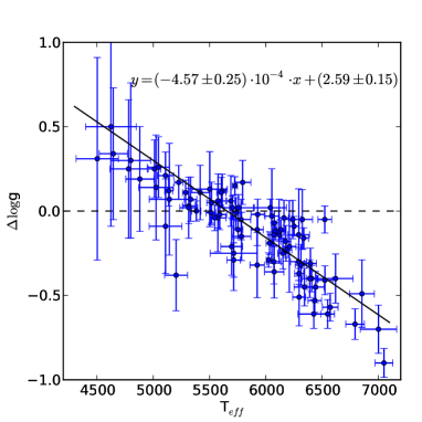
Figure 2: Surface gravity difference (‘photometric - spectroscopic’) versus the (unconstrained) effective temperature. A linear fit is shown with the solid black curve.

We fitted the trend with temperature with a linear function, taking into account the errors on both datasets (see Figure 2). We used the complete sample of 87 stars and followed the procedure as described in Numerical Recipes in C (Press et al., 1992) to obtain 1-sigma errors on the coefficients. We found the following relation:

$$\log g_{LC}-\log g_{spec}=-4.57\pm 0.25\cdot 10^{-4}\cdot T_{\mathrm{eff}}+2.59\pm 0.15$$ (3)

This formula is valid for stars with an effective temperature between $4500$ K and $7050$ K. It can be used to correct for the spectroscopic surface gravity when no transit light curve is available (and thus even for stars without planets). Using this formula assumes that the $\log g$ value coming from the transit is the more accurate one. As we will show later (see Section 4), these values can also suffer from inaccuracies. By applying this formula, we corrected our spectroscopic surface gravities for the sample of 87 stars (see Table 2). The resulting values compare, as expected, better with the photometric surface gravities.

As an additional test, we selected a subsample of our sample of stars, the ones with the highest S/N spectra (38 out of 87 stars). The coolest stars were hereby left out of the sample. We then again redid the spectroscopic analysis, but this time we fixed the surface gravity to the value corrected using Equation 3..

We compare the spectroscopic parameters obtained from fixing the surface gravity to the formula corrected value (’corr’) with the unconstrained spectroscopic parameters (’spec’) and the ones obtained from fixing the surface gravity to the photometric light curve value (’LC’). All parameters compare really well (see Figure 3), with mean differences of $13$ K, $0.02$ dex and $0.02$ km/s for the effective temperature, metallicity, and microturbulence, respectively for the difference between the corrected values and the spectroscopic values. For the differences between the corrected and the photometric results, we find mean differences of $-21$ K, $-0.01$ dex and $-0.06$ km/s for the effective temperature, metallicity, and microturbulence, respectively. No obvious trends are present. For completeness we calculated the MADs again. For the difference between the corrected values and the spectroscopic values, we find a MAD of $38$ K, $0.02$ dex and $0.08$ km/s for the effective temperature, metallicity, and microturbulence, respectively. The difference between the corrected values and the photometric values gives a MAD of $42$ K, $0.02$ dex and $0.08$ km/s for the effective temperature, metallicity, and microturbulence, respectively. These are thus well within the error bars.

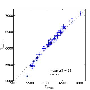
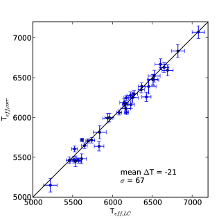
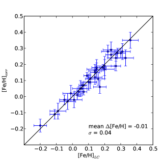
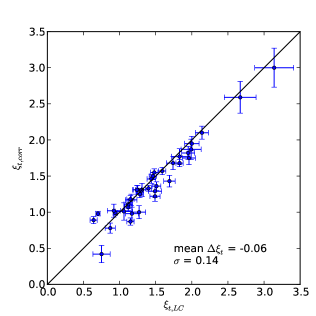
Figure 3: Comparisons of the spectroscopic effective temperatures, metallicities, and microturbulences (left to right). In the top panels we compare the unconstrained results (‘spec’) with the results using a fixed surface gravity from the correction formula (‘corr’). In the bottom panels the comparison is shown between the two fixed results ($\log g$ from transit (‘LC’) and $\log g$ from the formula (‘corr’)).

4 Surface gravity from asteroseismology

As Huber et al. (2013) showed, the surface gravities obtained through the stellar density from the transit light curve may also be less accurate when the eccentricity or the impact parameter of the transiting planet are under- or overestimated or fixed whilst fitting the light curve. Asteroseismic $\log g$’s on the other hand are more accurate. Although most of the planets from our sample in the previous Section have almost circular orbits, it is still worth, especially since Huber et al. (2013) show clear trends, to check if a similar relation can be found to correct spectroscopic surface gravities if one would use asteroseismic surface gravities.

We used a sample compiled from the literature for which the asteroseismic parameters, the maximum frequency $\nu_{max}$ and the large separation $\Delta\nu$, are precisely determined and we have access to high-resolution spectra with moderate to high signal-to-noise. In the end, we have a sample of 86 stars, subsamples of the samples in Chaplin et al. (2014) and Bruntt et al. (2010). The first work contains asteroseismic data obtained with the Kepler space telescope (Borucki et al., 2009). The latter compiles a sample of stars analysed with HARPS (Mayor et al., 2003).

Spectroscopic parameters for the sample of Chaplin et al. (2014) are gathered from Molenda-Żakowicz et al. (2013). Their work contains spectroscopic parameters for Kepler targets derived by several methods, one of which is our method with the linelist of Sousa et al. (2008) as described in Section 2. There are 74 stars in common. The 12 stars from Bruntt et al. (2010) have been spectroscopically analysed with our method either in previous works (Santos et al., 2005; Sousa et al., 2008; Tsantaki et al., 2013; Santos et al., 2013) or in this work.

For stars that were previously not yet analysed by our team, we gathered per star 40 spectra from the HARPS archives (taken from the long asteroseismology series). We shifted them to the reference frame and added them together. Given that these stars are bright, this gives for a high S/N spectrum in the end. We then analysed them following the method described in Section 2. The results are in Table 2.

The surface gravities of the final sample of 86 stars are then obtained through isochrone fitting using the PARSEC isochrones (Bressan et al., 2012) in the web interface for the Bayesian estimation of stellar parameters (for details, see da Silva et al., 2006). As input parameters we needed the large separation $\Delta\nu$, the maximum frequency $\nu_{max}$, the effective temperature T_eff, and the metallicity [Fe/H]. As Bayesian priors we assumed the lognormal initial mass function from Chabrier (2003) and a constant star formation rate.

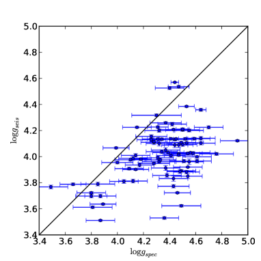
Figure 4: Asteroseismic versus spectroscopic surface gravity.

As expected, the spectroscopic and the asteroseismic surface gravities do not compare well (see Figure 4). As before, we redid, for most of the sample, the same spectroscopic analysis as performed in Mortier et al. (2013c), but this time we fixed the surface gravity to the asteroseismic value. The results can be found in Table 2.

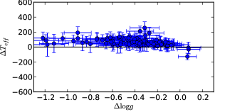
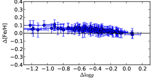
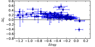
Figure 5: Differences of the spectroscopic results (left to right: effective temperature, metallicity, and microturbulence) as a function of the difference in $\log$g (defined as ‘constrained with asteroseismic $\log g$ - unconstrained’).

We compared the parameters obtained from fixing the surface gravity to the asteroseismic value with the parameters obtained with no constraints on the surface gravity. All parameters compare well, with mean differences of $68$ K, $0.04$ dex, and $0.15$ km/s for the effective temperature, metallicity, and microturbulence, respectively. In Figure 5, the differences in the spectroscopic parameters (defined as ‘constrained with asteroseismic $\log g$s - unconstrained’) are plotted against the difference in surface gravity (defined as ‘asteroseismic - spectroscopic’). All parameters are slightly anticorrelated with the difference in surface gravity, although most values stay within errorbars. Furthermore, we see the same converging trends as before.

Because of these trends, we again calculated the median absolute deviations (MAD) to quantify the variation. We find that the MADs are $28.5$ K, $0.02$ dex, and $0.06$ km/s for the effective temperature, metallicity, and microturbulence, respectively. Since these values are definitely within the errorbars of the parameters, these trends are thus small enough so that we are again confident that the surface gravity does not have a large effect on the determination of other atmospheric parameters using our method of spectral line analysis and the mentioned linelists. This result confirms the results from Section 3.

4.1 Correction with temperature

The differences in asteroseismic and spectroscopic surface gravity also seem to depend on the (unconstrained) effective temperature as can be seen in Figure 6, where a decreasing linear trend is again noticeable. The same trend is found for the microturbulence while comparing the $\log$g differences with metallicities reveals no additional trends.

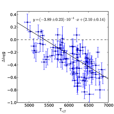
Figure 6: Surface gravity difference (‘asteroseismic - spectroscopic’) versus the (unconstrained) effective temperature. A linear fit is shown with the solid black curve.

We applied the same procedure as in Section 3.1 on the complete sample of 86 stars. We found the following relation:

$$\log g_{seis}-\log g_{spec}=-3.89\pm 0.23\cdot 10^{-4}\cdot T_{\mathrm{eff}}+2.10\pm 0.14$$ (4)

This formula is comparable to the fit presented in Section 3.1 for the overlapping temperature range ($5200$ K till $7000$ K). This may be somehow surprising since the transit $\log g$ may be less accurate than the asteroseismic one, as showed by Huber et al. (2013). However, we note that in our sample of transiting hosts, most planets have nearly circular orbits which strengthens the accuracy for the derived surface gravity through the transit light curve.

Given the better accuracy of asteroseismic surface gravities as compared to photometric surface gravities, we prefer Equation 4 to correct for the spectroscopic surface gravity. Since we barely have asteroseismic data for stars cooler than 5200 K, we cannot guarantee the accuracy of this formula for that temperature range and Equation 3 may thus be preferred for cooler stars.

5 Summary and discussion

In this work we derived spectroscopic parameters (effective temperature, metallicity, surface gravity and microturbulence) for a sample of FGK dwarfs in several ways. First we left the surface gravity free in the spectroscopic analysis as described in Section 2 (for the values, see Mortier et al., 2013c; Molenda-Żakowicz et al., 2013, and this work). Afterwards, we reran the same analysis whilst fixing the surface gravity to different values:

• A value obtained through the photometric transit light curve.

• A value obtained through the large separation and maximum frequency from asteroseismology.

• A value obtained through an empirical formula, using the effective temperature and the unconstrained surface gravity.

We find that, in almost all cases, the resulting stellar atmospheric parameters ($T_{\mathrm{eff}}$, [Fe/H], $\xi_{t}$) compare well within errorbars although there are slight trends noticable which correlate with the difference in surface gravity. The trends quickly converge and the differences in atmospheric parameters stay stable even for very large differences in surface gravity.

Differences between the constrained and the unconstrained atmospheric parameters can lead to differences in the values for the stellar mass and radius, and thus the planetary mass and radius. On average, the difference for the efffective temperature is about $70$ K and for the metallicity about $0.04$ dex. Using these numbers and the calibration formulae from Torres et al. (2010), we find that the resulting stellar mass and stellar radius will, on average, only differ by about $2-3\%$ and $1-1.5\%$, respectively, for FGK dwarfs. This will lead to an average difference of $1.3-2\%$ and $1-1.5\%$ for the planetary mass and radius. These differences are well within the precision that can currently be achieved (e.g. Huber et al., 2013).

It seems that the difference between the spectroscopic surface gravities and the photometric or asteroseismic ones is dependent on the effective temperature. By fitting a linear relation to the data, we obtained a correction formula for the surface gravity obtained with our spectroscopic method. Since asteroseismic surface gravities are the most accurate, we recommend to use Equation 4 rather than Equation 3. For stars cooler than 5200 K, we have little asteroseismic data and as such we cannot guarantee the accuracy of the formula for cooler stars. However, since Equation 3 from the photometric $\log g$s is comparable to the one coming from asteroseismic $\log g$s, the former may be used with caution for the cooler stars.

We note that although the surface gravity as calculated through these formulas may be more accurate, it cannot be more precise than the original unconstrained surface gravity, since the error bars of the spectroscopic $\log g$ are factored in when calculating the corrected value for $\log g$. Regardless, the value will definitely be more accurate than the one from the unconstrained MOOG analysis using our proposed linelists. As such the corrected value is better used for calculating other stellar parameters like the stellar mass and radius in case no additional methods can be used to derive the surface gravity, such as a transit light curve or asteroseismology.

For the other spectroscopic parameters the question remains whether the original spectroscopic parameters are accurate and can thus be used without performing the spectroscopic analysis again. In the case of the effective temperature, we compared our values with values obtained with the accurate and trusted InfraRed Flux Method (IRFM). We have 19 values from the transit sample from Maxted et al. (2011) and 21 from Casagrande et al. (2011) of which 2 from the transit sample and 19 from the asteroseismic sample. The comparisons can be seen in Figure 7.

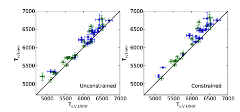
Figure 7: Comparisons of the unconstrained (left) and constrained (right) spectroscopic temperatures with literature temperatures obtained through the IRFM method (taken from Maxted et al. (2011), represented by green triangles, and Casagrande et al. (2011), represented by blue circles).

For stars cooler than 6300 K, the results compare well. We find mean differences of $-75\pm 100$ K and $-66\pm 74$ K, for our unconstrained and constrained temperatures, respectively. For the total sample, we find mean differences of $-106\pm 122$ K and $-122\pm 138$ K, respectively. For both the unconstrained and the constrained values, the hotter stars show larger differences, where the spectroscopic temperatures are larger than the ones from the IRFM. This may be an effect of the linelist used for the spectral line analysis. This linelist was calibrated for solar-like stars and the resulting effective temperatures may be overestimated for stars that are much hotter than our Sun (see also Sousa et al., 2011).

Given on one hand the marginal difference between comparing the IRFM temperatures with the constrained or the unconstrained temperatures and on the other hand the fact that fixing the surface gravity barely affects the other atmospheric parameters, we can be confident about the results of our unconstrained spectroscopic analysis for the derivation of the effective temperature, metallicity, and microturbulence of FGK dwarfs.

Torres et al. (2012) did a similar analysis, but they used an analysis based on synthetic spectra. As already mentioned in Section 3, our results are better constrained than those from an analysis with synthetic spectra and the linelist of Valenti & Fischer (2005). They found a linear relation between the temperature and metallicity differences with the surface gravity difference. For surface gravity differences $\Delta\log g\sim 0.5$ dex, they found differences in temperature of about 350 K and in metallicity of about 0.20 dex. With our spectral line analysis method and the carefully selected linelist, we have differences of only 120 K and 0.05 dex for temperature and metallicity, respectively.

To conclude, when atmospheric stellar parameters of FGK dwarfs are derived with high-resolution spectroscopy using our ARES+MOOG method, as described in Santos et al. (2013, and references therein), and the linelist of Sousa et al. (2008) or Tsantaki et al. (2013), we are confident that the resulting effective temperature, metallicity, and microturbulence are accurate and precise. The less accurate surface gravity can then easily be corrected using Equation 4 (or Equation 3 for the coolest stars). This method will always work with high-resolution spectra, even when no other means are available for the determination of surface gravity, like a transit light curve or asteroseismology.