Damped reaction field method and the accelerated convergence of the real space Ewald summation.

Abstract

In this paper we study a general theoretical framework which allows to approximate the real space Ewald sum by means of effective force shifted screened potentials, together with a self term. Using this strategy it is possible to generalize the reaction field method, as a means to approximate the real space Ewald sum. We show that this method exhibits faster convergence of the Coulomb energy than several schemes proposed recently in the literature while enjoying a much more sound and clear electrostatic significance. In terms of the damping parameter of the screened potential, we are able to identify two clearly distinct regimes of convergence. Firstly, a reaction field regime corresponding to the limit of small screening, where effective pair potentials converge faster than the Ewald sum. Secondly, an Ewald regime, where the plain real space Ewald sum converges faster. Tuning the screening parameter for optimal convergence occurs essentially at the crossover. The implication is that effective pair potentials are an alternative to the Ewald sum only in those cases where optimization of the convergence error is not possible.

I Introduction

The increasing availability of large scale computer facilities is allowing to study ever more complicated systems, with greater detail as well as longer length and time scales. Despite this progress, the accurate evaluation of electrostatic interactions remains the most important bottleneck in molecular simulations of charged systems.Allen and Tildesley (1987); Frenkel and Smit (2002)

This uncomfortable situation is reflected in the number of different alternatives which are available in the literature in order to deal with Coulombic interactions.Barker and Watts (1973); de Leeuw et al. (1980); Lekner (1989); Hummer et al. (1992); Darden et al. (1993); Wolf et al. (1999); Tyagi (2005); Shan et al. (2005); Fennell and Gezelter (2006) Yet, it is clear that the benchmark for both efficiency and accuracy of all studies remain the Ewald summation technique.Esselink (1995); Toukmaji and Board (1996); Hummer et al. (1999)

In this method, the full electrostatic energy of the system is split into a real space contribution, which amounts to a pairwise summation of an effective damped Coulomb potential, and a Fourier contribution, which embodies the long range effects of the Coulomb interactions. The latter term features a Fourier transform of the charge distribution, which on the one hand, brings some conceptual difficulties,de Leeuw et al. (1980); Smith (1981); Hummer et al. (1999); Ballenegger (2014) and on the other, is very time consuming to calculate.Kolafa and Perram (1992)

In the last decade, a number of studies have been devoted to study more or less efficient methodologies that allow to calculate electrostatic interactions while avoiding the cumbersome Fourier contributions of the Ewald sum.Wolf et al. (1999); Zahn et al. (2002); Fennell and Gezelter (2006); Fukuda et al. (2011); Hansen et al. (2012); Fukuda (2013) Such techniques, named recently under the provocative name of pairwise alternatives to the Ewald sum, have recently received considerable popularity, but also some degree of controversy as regards efficiency,Hansen et al. (2012) and accuracy.Mendoza et al. (2008); Muscatello and Bresme (2011)

The fact is that a pairwise alternative to the Ewald summation has been available ever since the first few simulations of Coulombic systems.Barker and Watts (1973); Neumann (1983); Barker (1994) Indeed, the Reaction Field Method is almost as old as computer simulations of charged systems,Allen and Tildesley (1987) yet, it has a clear theoretical background which more recent approaches lack completely.Zahn et al. (2002); Fennell and Gezelter (2006); Hansen et al. (2012) Despite this situation, the Reaction Field Method seems to have been largely abandoned in favor of other techniques, with some exceptions.Miguez et al. (2010)

Recently, Fukuda et al. proposed a heuristic approach to approximate the Coulomb sum. This approach shares advantages of some of the pairwise methods, in the sense that it screens the Coulomb interactions with a fast decaying function, but has a somewhat more elaborate electrostatic background.Fukuda et al. (2011) Indeed, it has been recently recognized that this approach may be considered as a generalization of the reaction field method to screened potentials.Kamiya et al. (2013)

In this work we attempt to provide a sound theoretical background for a generalized reaction field method that achieves fast convergence of the Coulomb sum as with several of the most popular pairwise alternatives.Wolf et al. (1999); Fennell and Gezelter (2006) The theoretical calculations are supplemented with numerical results for test systems, which demonstrate the superiority of reaction field methods. Additionally, we perform detailed analysis of the Coulomb sum convergence error for either reaction field and Ewald methods. This will allow us to identify the region of convergence parameters where each method is advantageous.

II Theoretical Background

II.1 Ewald Summation

In most simulations of charged systems, the influence of long range electrostatic interactions is estimated by assuming the finite sample is surrounded by an infinite number of replicas. The energy felt by, say, charge $i$, may be then estimated as a lattice sum over the replicas:

$$U_{i}=\sum_{{\bf n}={0}}\sum_{j}^{\prime}\frac{q_{i}q_{j}}{|\mathbf{r}_{ij}+{\bf n}|}$$ (1)

where ${\bf n}$ denotes a translation of the unit cell vector, $q_{i}$ is the charge on particle $i$, and $\mathbf{r}_{ij}$ is the position of $j$ relative to $i$. Furthermore, it is understood that the first sum runs over all possible unit cell translations, while the second sum runs over all charges inside the unit box. A prime reminds that $j$ must be different from $i$ when ${\bf n}={\bf 0}$.

This trick only gets rid of the boundary problem, but not of the actual calculation of $U_{i}$, since the series is known to be conditionally convergent, with a very slow convergence in the favorable cases. A particularly inconvenient case is a summation over spherical shells, which is often not convergent.de Leeuw et al. (1980); Wolf et al. (1999)

In the classical treatment of Ewald, the conditionally convergent lattice sum of charges is transformed into two rapidly convergent series, such that:

$$U_{i}=U^{\rm R}_{i}+U^{\rm F}_{i}$$ (2)

with

$$U^{\rm R}_{i}=\sum_{{\bf n}={0}}\sum_{j}^{\prime}q_{i}q_{j}\frac{\mathrm{e}rfc(\alpha|\mathbf{r}_{ij}+{\bf n}|)}{|\mathbf{r}_{ij}+{\bf n}|}$$ (3)

and

$$U^{\rm F}_{i}=4\pi\sum_{{\bf k}\neq{\bf 0}}\rho(\mathbf{k})\frac{e^{-\frac{k^{2}}{4\alpha^{2}}}}{k^{2}}q_{i}e^{-i\mathbf{k}\cdot\mathbf{r}_{i}}-q_{i}^{2}\frac{\alpha}{\sqrt{\pi}}$$ (4)

where $\mathbf{k}$ are vectors in Fourier space and $\rho(\mathbf{k})$ is the Fourier transform of the charge density. Additionally, the Ewald sum may contain a surface term, $U_{\rm surf}$, which accounts for the boundary conditions of the system. Such term arises strictly from the long range electrostatic interactions with the boundary and surrounding medium, and is therefore essentially a Fourier contribution corresponding to the missing $k=0$ term of the reciprocal space sum.de Leeuw et al. (1980); Smith (1981); Ballenegger (2014) In practice, for bulk systems under metallic boundary conditions the surface term may be neglected, so that we will henceforth drop this complication.

The inverse length, $\alpha$, plays a key role, dictating the convergence of the series. A large value of $\alpha$ leads to a rapidly convergent real space series that can be actually truncated already at ${\bf n}=0$, but then the $U^{\rm F}$ contributions converges slowly. Alternatively, a small value of $\alpha$ produces a very fast convergence of $U^{\rm F}$, but then $U^{\rm R}$ is slowly convergent.

An important observation made by Wolf et al. is that for moderately small values of $\alpha$, most of the Fourier contribution is actually given by the simple self term,

$$U^{\rm self}=-q_{i}^{2}\frac{\alpha}{\sqrt{\pi}},$$ (5)

so that the expensive reciprocal space summation may be ignored altogether.Wolf et al. (1999)

This observation has allowed for the recent development of efficient methodologies for the calculation of electrostatic interactions.Wolf et al. (1999); Zahn et al. (2002); Fennell and Gezelter (2006); Fukuda et al. (2011)

II.2 Accelerating the convergence of the real space sum

Having circumvented the problem of calculating the expensive reciprocal space sum, there still remains a crucial issue: how fast is the convergence of $U^{\rm R}$ in those cases where the reciprocal space summation may be ignored?

For most practical purposes, $\mathrm{e}rfc(\alpha r)$ decays so fast that the lattice summation required for the evaluation of $U_{i}^{\rm R}$ may be ignored. Rather, a plain spherical cutoff is usually employed for distances larger than a cutoff radius, $R_{c}$, with the hope that terms of order $\mathrm{e}rfc(\alpha R_{c})$ or smaller may be neglected. However, it remains desirable to have a cutoff as small as possible. For this purpose, one may try to exploit the techniques of continuum electro–dynamics for the $\mathrm{e}rfc(\alpha r)/r$ potential in the same spirit as it has been successfully done for the plain Coulomb potential.Barker and Watts (1969); Neumann (1983); Hummer et al. (1992); Wolf et al. (1999) This would allow to truncate $U_{i}^{\rm R}$ at cutoffs where $\mathrm{e}rfc(\alpha r)$ is actually not negligible.Wolf et al. (1999); Zahn et al. (2002); Fennell and Gezelter (2006); Fukuda et al. (2011)

$\leftarrow$

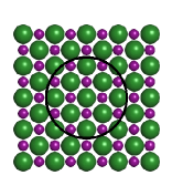
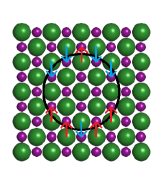
$\rightarrow$

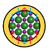
Figure 1: Sketch of the charge neutralization schemes employed in the Wolf and Damped Reaction Field methods. In the Wolf method (left), the net charge inside the sphere surrounding the central ion is uniformly spread over its surface. In the Damped Reaction Field Method (right), an additional surface charge due to broken effective dipoles between the central ion and the surrounding charges is considered. For a perfectly regular crystal lattice, the charge distribution is also uniform, but will usually be non-uniform and therefore produce a net force.

In this regard, another important observation made by Wolf is that Coulomb sums over spherical shells show good convergence whenever the net charge inside the sphere vanishes (Fig. 1).Wolf (1992) Whence, the poor convergence is due to the the fact that spheres of arbitrary radius centered about an ion $i$ will usually carry a net charge, $\Delta q_{i}$. The convergence of the Coulomb sum over spheres can be much improved by summing over charge neutralized spheres. This may be achieved in practice by assuming a fictitious uniform charge $\sigma_{i}^{\rm charge}$ over the surface of the sphere:Wolf et al. (1999)

$$\sigma_{i}^{\rm charge}=\frac{1}{4\pi R_{c}^{2}}\sum_{j}^{*}q_{j}$$ (6)

where the asterisk superscript indicates that the summation is restricted to those particles $j$ inside the cutoff sphere (such that $r_{ij}<R_{c}$).

Whence, for a source charge $i$ with arbitrary electric potential $q_{i}\phi(r)$, an improved approximation for the energy is:

$$U_{i}\approx\sum_{j}^{*}q_{i}q_{j}\phi(r_{ij})-q_{i}\Delta q_{i}\phi(R_{c})$$ (7)

Surprisingly, this charge neutralization may be implemented by means of an effective pairwise potential:Wolf et al. (1999)

$$u=q_{i}q_{j}\{\phi(r_{ij})-\phi(R_{c})\}$$ (8)

where the first term in the right hand side accounts for the bare interaction from the potential $q_{i}\phi(r)$, while the second term is the energy resulting from the interaction with the fictitious charge distribution of Eq. (6). Clearly, such interaction merely shifts the pair potential. Therefore, it does not result in an additional force.

However, one expects that the truncation of interactions at $R_{c}$ will not only produce a spurious net charge about ion $i$, but also a net polarization (Fig. 1).Wolf (1992) The force stemming from the uniform net charge is zero for reasons of symmetry, but the net polarization will result in a finite electric field on charge $i$.Fukuda et al. (2011)

This idea may be elaborated quantitatively in terms of the sphere’s polarization and the laws of electrostatics, which dictate that a polarized dielectric produces a surface charge density of magnitude:

$$\sigma_{i}^{\rm pol}({\bf e})={\bf P_{i}}\cdot{\bf e}$$ (9)

where ${\bf P}_{i}$ is the net polarization inside the sphere of radius $R_{c}$ centered on $i$ and ${\bf e}$ is a unit vector normal to the surface. Since the medium is overall neutral, we assume that the charges beyond the sphere act such as to cancel exactly this charge distribution. Accordingly, the full charge neutralizing distribution is:

$$\sigma_{i}^{\rm neutral}=-(\sigma_{i}^{\rm charge}+\sigma_{i}^{\rm pol}({\bf e}))$$ (10)

The particle $i$ bears a potential $\phi(r)$, and thus exerts a force $-\nabla\phi(r)$ on whichever other charge. Now, consider the infinitesimal force, $\mbox{$\,$}\mathrm{d}{\bf F}_{i}^{\rm surf}$ felt by charge $i$ due to the charge neutralizing distribution on an infinitesimal surface element $\mbox{$\,$}\mathrm{d}S=R^{2}\sin\theta\mbox{$\,$}\mathrm{d}\theta\mbox{$\,$}\mathrm{d}\phi$:

$$\mbox{$\,$}\mathrm{d}{\bf F}_{i}^{\rm surf}=-q_{i}\left.\nabla\phi\;\right|_{R_{c}}\;\sigma_{i}^{\rm neutral}\mbox{$\,$}\mathrm{d}S$$ (11)

Integrating over all the sphere’s surface, the term stemming from the uniform distribution $\sigma_{i}^{\rm charge}$ vanishes for reasons of symmetry, but the non uniform $\sigma_{i}^{\rm pol}({\bf e})$ term yields:

$${\bf F}_{i}^{\rm surf}=\frac{4\pi}{3}q_{i}\left.\frac{\mbox{$\,$}\mathrm{d}\phi}{\mbox{$\,$}\mathrm{d}r}\;\right|_{R_{c}}R_{c}^{2}\;{\bf P}_{i}$$ (12)

After substitution of ${\bf P_{i}}$ in terms of the explicit charges inside the sphere we obtain:

$${\bf F}_{i}^{\rm surf}=q_{i}\sum_{j}^{*}q_{j}\left.\frac{\mbox{$\,$}\mathrm{d}\phi}{\mbox{$\,$}\mathrm{d}r}\;\right|_{R_{c}}\frac{r_{ij}}{R_{c}}\frac{\mathbf{r}_{ij}}{r_{ij}}$$ (13)

The total force effectively felt on $i$ then contains the actual interactions between particles inside the sphere, together with the surface term accounting effectively for interactions with the remaining charges:

$${\bf F}_{i}=-\sum_{j}^{*}q_{i}q_{j}\left.\nabla\phi\right|_{r_{ij}}+q_{i}\sum_{j}^{*}q_{j}\left.\frac{\mbox{$\,$}\mathrm{d}\phi}{\mbox{$\,$}\mathrm{d}r}\right|_{R_{c}}\frac{r_{ij}}{R_{c}}\frac{\mathbf{r}_{ij}}{r_{ij}}$$ (14)

Clearly, the net force may be cast in terms of an effective pair potential of the form:

$${\bf F}_{ij}=-q_{i}q_{j}\left(\left.\frac{\mbox{$\,$}\mathrm{d}\phi}{\mbox{$\,$}\mathrm{d}r}\right|_{r_{ij}}-\left.\frac{\mbox{$\,$}\mathrm{d}\phi}{\mbox{$\,$}\mathrm{d}r}\right|_{R_{c}}\frac{r_{ij}}{R_{c}}\right)\frac{\mathbf{r}_{ij}}{r_{ij}}$$ (15)

This is the formal result we sought for. It corresponds to a continuous linearly screened force which smoothly vanishes at the cutoff.

II.3 Discussion

In order to understand its significance, it is convenient to recall the result for the effective electrostatic potential of the Reaction Field Method, which assumes a continuous dielectric medium with dielectric constant $\epsilon$ beyond the cutoff:Neumann (1985)

$${\bf F}_{ij}=q_{i}q_{j}\left(\frac{1}{r_{ij}^{2}}-\frac{2\epsilon-2}{2\epsilon+1}\frac{1}{R_{c}^{2}}\frac{r_{ij}}{R_{c}}\right)\frac{\mathbf{r}_{ij}}{r_{ij}}$$ (16)

Comparing this result with Eq. (15), it is clearly seen that our result is recovered for the special case where $\phi(r)=1/r$, as in the Coulomb potential, and the additional assumption of $\epsilon=\infty$. Whence, Eq. (15) corresponds to a generalization of the Reaction Field Method for arbitrary electric potentials, and a particular choice for the boundary conditions at the surface of the cutoff sphere. The Reaction Field Method shows that taking into account explicitly a finite susceptibility beyond the cutoff requires to assume a surface charge density of $\sigma_{i}^{\rm pol}=(2\epsilon-2)/(2\epsilon+1){\bf P_{i}}\cdot{\bf e}$ in place of Eq. (9).

On the other hand, the assumption embodied in Eq. (9), and other methods,Wolf et al. (1999); Fukuda et al. (2011); Fukuda (2013) implies that the charges left out beyond the cutoff are fully available to screen the net dipole created inside the sphere. This statement may be understood if we consider yet another refinement over the Reaction Field Method, namely, to assume that the charge distribution outside the cutoff sphere is given as a Boltzmann weighted average dictated by the field of the ions inside the sphere. This task may be accomplished in the Debye-Hückel approximation, and yields a generalization of the Reaction Field Method that accounts for interactions with both a dielectric continuum and a smooth charge distribution of given concentration:Barker (1994); Tironi et al. (1995)

$${\bf F}_{ij}=q_{i}q_{j}\left(\frac{1}{r_{ij}^{2}}-\frac{(2\epsilon-2)(1+\kappa R_{c})+\epsilon(\kappa R_{c})^{2}}{(2\epsilon+1)(1+\kappa R_{c})+\epsilon(\kappa R_{c})^{2}}\frac{1}{R_{c}^{2}}\frac{r_{ij}}{R_{c}}\right)\frac{\mathbf{r}_{ij}}{r_{ij}}$$ (17)

where $\kappa$ is the inverse Debye screening length of the free charges. For vanishing concentration of charges, $\kappa=0$, and this model recovers Eq. (16) exactly. In the opposite limit, $\kappa$ becomes infinite, and then Eq. (17) becomes equal to the Reaction Field Method with conducting boundary conditions. This illustrates our statement, that the approximation Eq. (9) corresponds to an infinite availability of charges for screening of the dipole inside the cutoff sphere. Unfortunately, the accuracy of Debye-Hückel theory is limited to very low ion concentration, so the refinement of Eq. (17) is more a conceptual improvement than an accurate working equation at typical simulation conditions.

The fact is, once the interactions are truncated beyond a cutoff, one can not do without an arbitrary approximation as to the charge distribution of the surrounding medium. The first obvious choice is to assume a dielectric response, but then the precise value of the dielectric constant needs to be specified. In simulations of molten salts or ionic fluids, it seems reasonable to choose metallic boundary conditions. On the other hand, in simulations of polar fluids the choice of $\epsilon$ equal to the fluid’s dielectric constant is more natural. If, however, the polar fluid is simulated with explicit charges, as is usually the case, there is then not an obvious choice.

Fortunately, most solvents of interest in studies of charged systems, and particularly water, have a rather large dielectric constant, so that the ratio $(2\epsilon-2)/(2\epsilon+1)$ is very close to unity, as in the case of $\epsilon=\infty$. Furthermore, for finite $\epsilon$, the force of the RFM becomes discontinuous at the cutoff, and this severely hampers applications in Molecular Dynamics. Such inconvenience may be altogether avoided, since it has been shown that the precise choice of dielectric boundary conditions does not significantly change the outcome of the simulations, particularly for the case of phase coexistence.Garzon et al. (1994); Miguez et al. (2010)

For these reasons, we believe the boundary conditions that are implied in Eq. (15) are the most judicious choice for condensed phases of both i) polar fluids with high dielectric constant and ii) molten salts that will be studied in the next section. Indeed, they correspond to the accepted choice in a large body of simulations.Garzon et al. (1994); Wolf et al. (1999); Miguez et al. (2010); Fukuda et al. (2011); Fukuda (2013) A word of caution is required for applications to very low density systems. In such cases, where typically ions are separated by large distances and the Debye screening length is very large, one cannot expect that the net charge about a single isolated ion will be neutralized at all within a small cutoff. In such cases, an Ewald type summation might be the only reliable alternative.

II.4 Damped force

The advantage of Eq. (15) over the traditional RFM is that it allows to accelerate the convergence by using a fast decaying electric field $\phi(r)$ in place of the Coulomb potential.

For $\phi(r)=\mathrm{e}rfc(\alpha)/r$, it yields a generalized damped reaction field equation for the force, as:

$$F_{ij}=q_{i}q_{j}\left\{\left[\frac{\mathrm{e}rfc(\alpha r_{ij})}{r_{ij}^{2}}+\frac{2\alpha}{\sqrt{\pi}}\frac{e^{-\alpha^{2}r_{ij}^{2}}}{r_{ij}}\right]-\left[\frac{\mathrm{e}rfc(\alpha R_{c})}{R_{c}^{2}}+\frac{2\alpha}{\sqrt{\pi}}\frac{e^{-\alpha^{2}R_{c}^{2}}}{R_{c}}\right]\frac{r_{ij}}{R_{c}}\right\}$$ (18)

For the special case where $\alpha=0$, we recover the result of Eq. (16) with $\epsilon=\infty$.

It is difficult here to know exactly how Eq. (18) is related to the corresponding expressions given by Wolf et al.Wolf et al. (1999) The reason is that these authors obtain their forces unconventionally as an imaginary process where $r_{ij}\to R_{c}$ in order to enforce their potential to yield a shifted force, which would otherwise not be the case. Whence the authors write:

$$F_{ij}=q_{i}q_{j}\left\{\frac{1}{r_{ij}^{2}}-\frac{1}{R_{c}^{2}}\left.\frac{r_{ij}}{R_{c}}\right|_{r_{ij}=R_{c}}\right\}$$ (19)

We find difficult to interpret what the condition $r_{ij}=R_{c}$ means. If we simply ignore the odd condition, we recover Eq. (15). If, as interpreted by Fennell and Gezelter, we take the equality as written, we then obtain merely a shifted force potential of little electrodynamic significance.Fennell and Gezelter (2006)

II.5 Formal treatment

In the previous section we have obtained our results using elementary electrodynamics and back of the envelope arguments. Here we derive our results using a more formal treatment of molecular electrodynamics as formulated by Neumann, Boresch and Steinhauser.Neumann (1983); Boresch and Steinhauser (2001)

Our derivation starts with a basic equation for the electric field that results from the polarization ${\bf E}({\bf r})$ of a uniform medium due to an external source field, ${\bf E_{0}}$:

$${\bf E}(\mathbf{r})={\bf E_{0}}(\mathbf{r})+\int\mbox{$\,$}\mathrm{d}\mathbf{r}^{{}^{\prime}}{\bf T}(\mathbf{r}-\mathbf{r}^{{}^{\prime}})\cdot{\bf P}(\mathbf{r}^{{}^{\prime}})$$ (20)

where ${\bf T}(\mathbf{r})=\nabla\nabla\phi$ is the dipole–dipole tensor, and the integration is over the simulation cell under toroidal boundary conditions. This equation was instrumental in the establishment of a consistent framework for the calculation of dielectric relaxation phenomena in the 1980’s,Neumann (1983); Neumann et al. (1984) and has been exploited recently to study the dielectric constant of anisotropic media.MacDowell and Vega (2010)

An important point here is the realization that this equation is also valid for the case where ${\bf E_{0}}(\mathbf{r})$ results from atomic charge distributions interacting via a generalized Green’s function $\phi(\mathbf{r})$, whether it is a Coulomb interaction or some other modified central force potential. The only caution is to keep in mind that the dipole–dipole tensor has to be accordingly modified as in the definition above. Taking these two considerations into account, we can write an equation for the electric field on charge $\mathbf{r}_{i}$ that results from the presence of a second charge $\mathbf{r}_{j}$ interacting with $i$ via the generalized green function $\phi_{\rm mod}(r)=S(r)/r$, with $S(r)$ an arbitrary function:Boresch and Steinhauser (2001)

$${\bf E}(\mathbf{r}_{i})=-\nabla\phi_{\rm mod}(r_{ij})+\int\mbox{$\,$}\mathrm{d}\mathbf{r}{\bf T}_{\rm mod}(\mathbf{r}_{i}-\mathbf{r})\cdot{\bf P}(\mathbf{r})$$ (21)

where now ${\bf T}_{\rm mod}(\mathbf{r}_{i})=\nabla\nabla\phi_{\rm mod}(r)$. For our purposes, it proves convenient to express ${\bf T}_{\rm mod}$ in terms of the dipole–dipole tensor corresponding to a Coulomb potential:Boresch and Steinhauser (2001)

$${\bf T}_{\rm mod}=(S-rS^{\prime}+\frac{1}{3}r^{2}S^{\prime\prime}){\bf T}+\frac{1}{3}\frac{S^{\prime\prime}}{r}{\bf I}$$ (22)

where ${\bf I}$ is a unit matrix and the prime indicates derivation with respect to $r$.

In order to perform the integral of Eq. (21), one needs to take into account that ${\bf T}(\mathbf{r})$ is an odd function, except at the singularity $\mathbf{r}\to{\bf 0}$, where the tensor is:Neumann (1983)

$$\lim_{r\to 0}{\bf T}(\mathbf{r})=-\frac{4\pi}{3}\delta(\mathbf{r})$$ (23)

As a result, the integral does not vanish altogether, but rather, yields:

$${\bf E}(\mathbf{r}_{i})=-\nabla\phi_{\rm mod}(r_{ij})-\frac{4\pi}{3}S(0)\;{\bf P}(\mathbf{r}_{i})+\frac{1}{3}\int\mbox{$\,$}\mathrm{d}\mathbf{r}\frac{S^{\prime\prime}}{r}\;{\bf I}\cdot{\bf P}(\mathbf{r})$$ (24)

this is a general result for a wide choice of $S$ functions, including whatever polynomial, the exponential or the complementary error function. The integral that remains is difficult to solve for the general case of a position dependent polarization. However, assuming constant polarization within the cutoff sphere, the integral can be solved by parts, yielding:

$${\bf E}(\mathbf{r}_{i})=-\nabla\phi_{\rm mod}(r_{ij})-\frac{4\pi}{3}\phi_{\rm mod}^{\prime}(R_{c})R_{c}^{2}\;{\bf P}_{i}$$ (25)

where ${\bf P}_{i}$ is the uniform polarization inside the sphere about $i$, that is, ${\bf P}_{i}=q_{j}\mathbf{r}_{ij}/4\pi R_{c}^{3}$. Substitution of ${\bf P}_{i}$ into the above result and multiplying by the charge $q_{i}$ at $i$ then leads right away to the general result obtained in the previous section, Eq. (15).

The significance of calculating an electric field rather than a potential can be now understood, since a continuous potential at $r=R_{c}$ results ab–initio by integration of the force:

$$u(r)=-\int_{\infty}^{r}F(r)\mbox{$\,$}\mathrm{d}r$$ (26)

considering that $F(r)$ vanishes beyond $R_{c}$, we obtain:

$$u(r_{ij})=q_{i}q_{j}\left\{\phi_{\rm mod}(r_{ij})-\phi_{\rm mod}(R_{c})-\frac{1}{2}\phi_{\rm mod}^{\prime}(R_{c})\;\frac{r_{ij}^{2}-R_{c}^{2}}{R_{c}}\right\}$$ (27)

Clearly, the resulting potential not only shifts $\phi_{\rm mod}(r)$ but also produces an additional polarization force (c.f. Eq. (8)). The equation has the form of a generalized reaction field potential, that may be employed to improve the summation of whatever generalized $\phi(r)$ function. For $\phi=1/r$ we recover the reaction field model of Neumann,Neumann (1983) properly modified to produce a continuous force at $r=R_{c}$ as in Ref.Hummer et al., 1992. This is an advantage over other treatments, where the continuous form is implemented add–hoc on the basis of numerical convenience (see DL-POLY or Gromacs reference manuals).

In order to complete the formulation, we further need to supplement our model with a self term that gauges the total energy, accounting for the difference between the actual and modified potentials:Boresch and Steinhauser (2001)

$$U_{i}^{\rm self}=\lim_{r\to 0}\quad\frac{1}{2}\;q_{i}^{2}\left(u(r)-\phi_{\rm mod}(r)\right)$$ (28)

Using Eq. (27), we obtain the general expression for the self term of the generalized reaction field method.

$$U_{i}^{\rm self}=-\frac{1}{2}\;q_{i}^{2}\left(\phi_{\rm mod}(R_{c})-\frac{1}{2}\;\phi^{\prime}_{\rm mod}(R_{c})R_{c}\right)$$ (29)

Eq. (27) and Eq. (29) are the more important results of this section. For the special case where $\phi(r)=1/r$, we recover exactly the reaction field model of Hummer et al.Hummer et al. (1992) Here, we show that the reaction field form is kept generally for whatever Green function $\phi_{\rm mod}(r)$. As a result, it may be exploited also to accelerate the convergence of damped coulomb potentials in Ewald type summations.

II.6 Pairwise schemes for the calculation of the real space Ewald summation

We finish this section with the pair potential and self terms that result for probably the most significant damped coulomb potential, namely, $\phi_{\rm mod}(r)=\mathrm{e}rfc(\alpha r)/r$. Using Eq. (27) and Eq. (29), we obtain:Elvira (2012)

$$u_{\rm ercf}(r_{ij})=q_{i}q_{j}\left\{\frac{\mathrm{e}rfc(\alpha r_{ij})}{r_{ij}}-\frac{\mathrm{e}rfc(\alpha R_{c})}{R_{c}}+\frac{1}{2}\left[\frac{\mathrm{e}rfc(\alpha R_{c})}{R_{c}^{2}}+\frac{2\alpha}{\sqrt{\pi}}\frac{e^{-\alpha^{2}R_{c}^{2}}}{R_{c}}\right]\frac{r_{ij}^{2}-R_{c}^{2}}{R_{c}}\right\}$$ (30)

While for the self term, we have:

$$U_{i}^{\rm self}=-\frac{1}{2}q_{i}^{2}\left\{\frac{\mathrm{e}rfc(\alpha R_{c})}{R_{c}}+\frac{1}{2}\left(\frac{\mathrm{e}rfc(\alpha R_{c})}{R_{c}}+\frac{2\alpha}{\sqrt{\pi}}e^{-\alpha^{2}R_{c}^{2}}\right)\right\}$$ (31)

Notice that this self energy corrects for the truncation of the exact real space lattice summation of $\phi_{\rm mod}(r)=\mathrm{e}rfc(\alpha r)/r$, Eq. (3). i.e., it cannot possibly account for the Fourier space term of Eq. (4). If the purpose is to approximate the full Coulomb sum, Eq. (1), and $\alpha$ is chosen such that the reciprocal space sum may be ignored, one must still account for the self term of the Fourier sum, Eq. (5).

Actually, this point can be illustrated from the formalism afforded by Eq. 21, 27, 28. To see this, consider the situation where this approach is applied to approximate the infinite sum Eq. (1) of coulomb potentials, $1/r$, instead of the related $\mathrm{e}rfc(r)/r$ sum of Eq. (3). Rather than employing Eq. (29) for the self term, we would then need to consider the self term as the limiting value of $-\frac{1}{2}q_{i}^{2}(u(r)-1/r)$, since now the excess energy is over $\phi=1/r$, rather than over $\phi_{\rm mod}=\mathrm{e}rfc(r)/r$. The self term would still be as Eq. (31), plus an extra term $\lim\,r\to 0$ of $-\frac{1}{2}\,q_{i}^{2}\,{\mathrm{e}rf}(r)/r$. One can recognize here exactly the self term of the Fourier contribution, Eq. (5). Therefore, the theoretical treatment provides naturally the generalized reaction field result of Eq. (30) and Eq. (31), plus the Ewald sum self term as the best possible approximation to Eq. (1) that can be obtained by performing a truncated sum of $\mathrm{e}rfc(r)/r$ terms.

The general results Eq. (27), Eq. (29), as well as Eq. (30)–Eq. (31) for the damped Coulomb potential are exactly as the Zero Charge-Zero Dipole method derived recently by Fukuda et al. using a heuristic approach based on the mirror image technique.Fukuda et al. (2011) Our results provide an alternative derivation showing clearly the strong connection with the Reaction Field technique.Hummer et al. (1992) As such, we will henceforth refer to Eq. (30)–(31) as Damped Reaction Field (DRF) Method.

The results Eq. (30)–(31) resemble effective pair potentials that have been suggested recently.Wolf et al. (1999); Zahn et al. (2002); Fennell and Gezelter (2006); Fukuda et al. (2011); Fukuda (2013) Indeed, they include a shift in the potential that is at the heart of Wolf’s method, but provide also an additional force as in the Fennel and Gezelter method and related approaches.Fennell and Gezelter (2006); Fukuda et al. (2011); Fukuda (2013)

In fact, all of these methods may be considered as a wide class, that, by use of Eq. 21, 27, 28, allows to approximate the real space Ewald summation of Eq. (3). This is achieved using an effective pairwise potential of the form:

$$u(r_{ij})=q_{i}q_{j}\left\{\begin{array}[]{cc}f(r_{ij};\alpha,R_{c})&\quad r_{ij}\leq R_{c}\\ 0&\quad r_{ij}>R_{c}\end{array}\right.$$ (32)

together with a self term:

$$U^{\rm self}_{i}=-\frac{1}{2}q_{i}^{2}g(\alpha,R_{c})$$ (33)

Table 1 provides a summary of different pairwise methods following the scheme above (Ref.Fukuda, 2013 also discusses the relation amongst different pairwise potential schemes). Recall that for the sake of approximating the full Coulomb sum, Eq. (1), the Fourier contribution Eq. (4) still needs to be evaluated. Under favorable cases, that may be achieved by neglecting all of the reciprocal space sum, and accounting only for the remaining self contribution, Eq. (5)).

However, the theoretical approach explained here shows that in practice all such methods may be also employed to accelerate the convergence of the real space summation alone, whether one opts to ignore the reciprocal space sum or not. Compared to other methodologies, however, our results have several advantages: 1) Both the potential and the force remain continuous at $r=R_{c}$; 2) The force and potential are fully consistent with each other, and are obtained in a straight forward manner (c.f. Ref. Wolf et al., 1999; Zahn et al., 2002) 3) The continuity of the expressions is not merely plugged in for numerical convenience, but results from a clear and well understood electrodynamic treatment (c.f. Ref. Fennell and Gezelter, 2006). 4) The self term is provided and follows systematically from the theoretical treatment (c.f. Ref. Fennell and Gezelter, 2006).

Pair potential	$f(r;\alpha,R_{c})$	$g(\alpha,R_{c})$	Limit $\alpha\to 0$
$u_{\rm Ew}$	$\phi(r)$	-	Coulomb
$u_{\rm Wolf}$	$\phi(r)-\phi(R_{c})$	$\phi(R_{c})$	Shifted Coulomb
$u_{\rm WFG}$	$\phi(r)-\phi(R_{c})-\phi^{\prime}(R_{c})(r-R_{c})$	$\phi(R_{c})-\phi^{\prime}(R_{c})R_{c}$	Force shifted Coulomb
$u_{\rm DRF}$	$\phi(r)-\phi(R_{c})-\frac{1}{2}\phi^{\prime}(R_{c})\frac{r^{2}-R_{c}^{2}}{R_{c}}$	$\phi(R_{c})-\frac{1}{2}\phi^{\prime}(R_{c})R_{c}$	Reaction Field

Table 1: List of pair potentials and self terms used to approximate the real space Ewald sum, Eq. (3), using the general scheme of Eq. (32)-Eq. (33), with $\phi(r)=\mathrm{e}rfc(\alpha r)/r$. The last column indicates the relation of each model to the Coulomb potential in the limit where $\alpha\to 0$. The entry $g(\alpha,R_{c})$ for $u_{\rm WFG}$ is the self term for the Wolf-Fennell-Gezelter method, not provided in the original reference.Fennell and Gezelter (2006) For the case where Eq. (32)-33 are employed to approximate the full Coulomb sum, Eq. (1), an extra self term, $2\frac{\alpha}{\sqrt{\pi}}$ accounting approximately for the Fourier contribution Eq. (4) must be added to $g(\alpha,R_{c})$.

III Results

In the following section, we will test the ability of different real–space lattice summations as a means to approximate the full electrostatic sum of Eq. (1). Whereas such methods are expected to provide a good convergence for dense fluids of dipolar molecules,Fennell and Gezelter (2006) we have chosen to study crystalline and molten ionic salts. This should provide a more stringent test than merely polar fluids and therefore allow us to obtain conclusions of more general validity.

As a test of an ordered ionic solid, we will consider crystalline sodium chloride. Accordingly, we will assume an ordered arrangement of + and - unit charges with lattice spacing $a$, as in the crystal rock salt lattice. For an ionic molten compound, we again consider configurations of + and - unit charges thermally sampled from a screened Yukawa fluid with hard sphere diameter $\sigma$.

The convergence of the average Coulomb energy felt by an ion is monitored by calculating:

$$U_{i}^{\rm R}(R_{c})=\sum_{j}^{*}u(r_{ij})+U^{\rm self}_{i}$$ (34)

with $u(r)$ and $U^{\rm self}_{i}$ as given by Eq. (32)-33, and the corresponding choice of $f(r;\alpha,R_{c})$ and $g(\alpha,R_{c})$ as indicated in Table 1 for different approximate schemes.

III.1 Charge neutralization schemes with no damping

In order to make a transparent comparison between DRF and Wolf’s charge neutralization schemes, let us first consider the case of zero damping, $\alpha=0$ so that $\phi$ adopts the bare Coulomb form $1/r$. In this case, Wolf’s charge neutralization scheme becomes a mere shifted Coulomb potential, while DRF becomes the Reaction Field Method.

Figures 2 and 3 show $U_{i}(R_{c})$ as estimated by bare Coulomb summation, Wolf’s method and DRF for solid NaCl and the 1:1 molten salt.

As expected, in the NaCl lattice (Fig. 2), the direct summation is not convergent, and the data is so scattered that it is not even possible to guess approximately the exact energy. The introduction of the neutralizing shell proposed by the Wolf’s method leads the energy to converge, and the amplitude of the oscillations decreases remarkably, even though the damping parameter is zero. However, if the DRF method is used instead, the amplitude of the oscillations decreases much more, to the point that they are hardly visible in the scale of the figure (at least beyond $R_{c}\approx 1.5a$). We have checked that this behavior also occurs for other crystalline structures, such as blende and CsCl.
The improved performance of charge neutralization schemes is also seen in the case of a molten ionic compound (Fig. 3). The only difference here is that the direct summation does converge, since, due to the lack of long-range order, the charges are effectively shielded. The convergence is, however, very slow. Again, the Wolf’s and DRF methods accelerate significantly the convergence, and DRF gives rise to somewhat smaller oscillations than Wolf’s method.

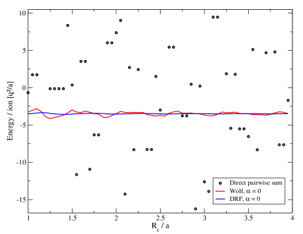
Figure 2: Electrostatic potential energy of the NaCl lattice calculated as the direct pairwise summation and by means of Wolf’s and DRF methods.

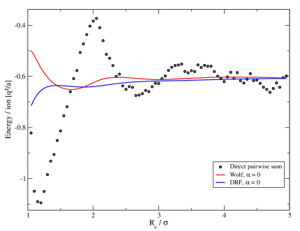
Figure 3: Electrostatic potential energy of a molten ionic compound of stoichiometry 1:1 calculated as the direct pairwise summation and by means of Wolf’s and DRF methods.

III.2 Role of damping

The convergence of $U_{i}(R_{c})$ may be much improved by using a damping function $\phi_{\rm mod}(r)=\mathrm{e}rfc(\alpha r)/r$. As noted above, choosing $\alpha=0$ transforms $\phi_{\rm mod}$ into the bare Coulomb potential. For finite $\alpha$, $\phi_{\rm mod}$ becomes a damped Coulomb potential with a decay rate that is governed by $\alpha$.

It is important to notice, however, that once $\alpha\neq 0$, then immediately the Fourier contribution to the Coulomb sum becomes finite, so that even in the limit $R_{c}\to\infty$, the sum $E_{i}(R_{c})$ is only an approximation for the full Coulomb sum.

As noted by Wolf, however, there is a wide choice of finite $\alpha$ where the only significant contribution to the Fourier sum, Eq. (4), is the self term, Eq. (5). For the NaCl crystal, for example, choosing $\alpha=1.0~{}a^{-1}$ the reciprocal space sum is $\approx 5\cdot 10^{-12}$ times smaller than the self term. The case of NaCl is however a particularly favorable one, and might not be always taken for granted. For another simple crystal structure such as CsCl, for example, the reciprocal space sum is now only $\approx 10^{-4}$ times smaller than the self term. A study of the structure factors reveals that CsCl is a very unfavorable case because here $\rho(\mathbf{k})$ vanishes only once every two $\mathbf{k}$ vectors, while NaCl is probably particularly favorable, since $\rho(\mathbf{k})$ vanishes for all but about n+1 every $(2n+1)^{3}$ $\mathbf{k}$ vectors.

For a fluid, the relative contribution of the sum cannot generally be determined, but one here expects that $\rho(\mathbf{k})$ is of finite range, and should therefore decay faster than for the case of CsCl.

Be as it may, one expects there to be a range of sufficiently small $\alpha$, where, on the one hand, the Fourier contribution is given essentially by the self term, while simultaneously, the convergence of the real sum is much improved. One then hopes that the reciprocal space sum can be ignored altogether, leaving all of the energy contribution in terms of a relatively fast decaying damped coulomb potential.

We test this hypothesis first for a perfect NaCl crystal, then for the 1:1 molten salt.

III.2.1 Perfect NaCl crystal

Figures 4 and 5 show the evolution of the real part of the energy of the NaCl crystal with the cut-off radius for finite $\alpha$ (1.0 $a^{-1}$ and 2.0 $a^{-1}$ respectively). Results are displayed for the real space Ewald summation (RSE), Wolf’s method (WM), Wolf-Fennell-Gezelter’s method (WFG) and DRF.

Notice that for finite $\alpha$, even the real part of the Ewald summation is convergent. However, the oscillations are rather large and exhibit discontinuities, while the convergence remains relatively slow. The use of Wolf’s method makes the oscillations decrease strongly. The DRF method shows a clear diminution of the oscillations of the energy, not only compared with RSE, but also with Wolf’s method, while the performance of WFG is about the same as that afforded by DRF. Further increasing $\alpha$ from $1.0~{}a^{-1}$ to $2.0~{}a^{-1}$ produces a spectacular improvement on the convergence of $U_{i}(R_{c})$. This is obvious right away by comparing both the $y$ and $x$ scales of figures 4 and 5. i.e., not only the asymptotic value of $U_{i}(R_{c})$ is reached much faster, but also the amplitude of the oscillations is decreased by more than an order of magnitude. Obviously, this is at the expense of making the Fourier contribution larger, and more importantly, increasing the relevance of the reciprocal space sum. In fact, for $\alpha=2.0~{}a^{-1}$ the reciprocal space sum is now already about $10^{-3}$ times the self term of Eq. (5), so that it becomes unsafe to approximate the Coulomb sum without taking account of the full Fourier contribution.

An interesting feature of both WFG and DRF is that, not only is the amplitude of the oscillations smaller, but also the discontinuities that were apparent in RSE and to a smaller extent in WM seem to be considerably smoothed. This smoothing property must be related to the presence of a shifted force contribution to the effective pair potential, since only WFG and DRF share this feature among the four methods tested. In fact, WFG and DRF perform similarly, so that it would seem it is the the shifted force contribution what makes these methods perform better than RSE and WM.

At this point it is convenient to mention the significance of the self term, Eq. (33). Indeed, at first thought one might consider that a constant contribution $U^{\rm self}_{i}$ merely shifts the total energy, but not the underlying dynamics so that it may be completely ignored. However, in order to compare the results of $U_{i}$ for different methods it is essential to account for the appropriate self contribution as indicated in Table 1. Actually, even for a given method, results with different $R_{c}$ (or $\alpha$) can only be compared when $U^{\rm self}_{i}$ is included. This is particularly relevant for the case of WFG, which does not include a self term in the original reference, and could only be compared with the RSE, WM and DRF by including the self term of Tab.1. This can also be of great importance in the simulation of open systems, as is the case of studies performed in the grand canonical ensemble.

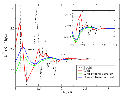
Figure 4: Evolution of the real part of the energy with the cut-off radius. NaCl perfect crystal. $\alpha=1.0~{}a^{-1}$.

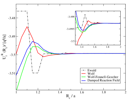
Figure 5: Evolution of the real part of the energy with the cut-off radius. NaCl perfect crystal. $\alpha=2.0~{}a^{-1}$.

As a final remark, we note the conclusions drawn from the analysis performed on NaCl also hold for other simple crystal structures such as CsCl and ZnS (not shown).

III.2.2 Molten salt

Let us now compare the performance of the pairwise summation schemes for the 1:1 molten salt.

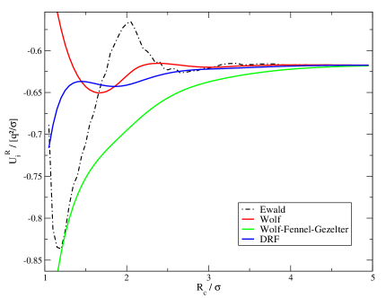
Figure 6: Evolution of the real part of the energy with the cut-off radius. Molten ionic compound of stoichiometry 1:1. $\alpha=0.4~{}\sigma^{-1}$.

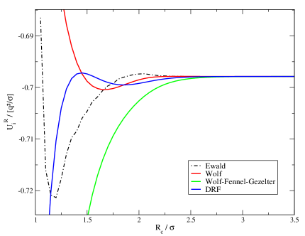
Figure 7: Evolution of the real part of the energy with the cut-off radius. Molten ionic compound of stoichiometry 1:1. $\alpha=1.0~{}\sigma^{-1}$.

Depicted in Figures 6 and 7 is the behavior of $U_{i}(R_{c})$ now calculated for a molten ionic compound. In a molten system, the oscillations of the energy are smoother than in a crystal, irrespective of the method used. Since the system is disordered, the interaction with new ions as the cut-off radius increases does not take place at discrete distances, but rather, continuously.
Nevertheless, the oscillations given by RSE are still too high, and the alternative pairwise schemes clearly improve this situation. In the figures, it is clear that Wolf’s method already diminishes widely the oscillations, and DRF makes this improvement somewhat more significant.
On the contrary, the WFG method now seems to converge slower, and more importantly, does not seem to oscillate but rather approach the asymptotic energy from below.

III.3 Calculation of the virial

In the preceding sections we have studied the convergence of the energy. Another important issue refers to the convergence of the forces. Since, however, the net force exerted on an ion in a perfect crystal is zero, we rather consider the virial per ion, which has similar convergence issues as the energy. Accordingly, we study the convergence of a virial function, defined as:

$$W_{i}^{R}(R_{c})=\sum_{j}^{*}w(r_{ij})$$ (35)

where

$$w_{ij}=\overrightarrow{f_{ij}}\cdot\overrightarrow{r_{ij}}$$ (36)

while the forces are given by differentiation of the corresponding pairwise potentials (c.f. Tab.1).

Figure 8 shows the evolution of the virial of an ion inside de NaCl lattice with the cut-off radius for a fixed value of $\alpha=1.0$. Results are shown for RSE, WFG, and DRF. Notice that we do not employ Wolf’s method here, as it gives a discontinuity in the force at $R_{c}$.

The figure explicitly shows a rather poor convergence of the RSE, which exhibits strong oscillations and discontinuities as a function of $R_{c}$. At this point, it is worth mentioning that for $\alpha=0$, the RSE method becomes the bare Coulomb sum and does also not converge at all (not shown). Using the effective pairwise schemes very much improves this situation. Indeed, the amplitude and also the frequency of the oscillations is reduced, while the convergence is also achieved faster. Apparently, WFG and DRF perform similarly, lending support to the idea that a shifted force is necessary (and perhaps sufficient) to improve the convergence of the sum. This is somewhat confusing, given that one can hardly attribute any electrostatic significance to the WFG scheme, which merely corresponds to a force shifted potential.

Figure 9 displays results for $W_{i}^{R}(R_{c})$ in the molten salt system, with $\alpha=0.4~{}\sigma^{-1}$. In this case, the direct RSE summation displays deviations of about the same amplitude than WFG and DRF, but clearly exhibits stronger discontinuities. Again both WFG and DRF perform similarly.

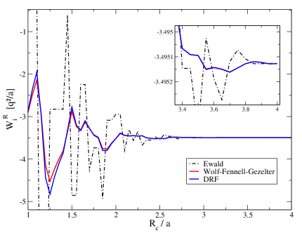
Figure 8: Evolution of the virial of an ion with the cut-off radius. NaCl perfect crystal. $\alpha=1.0~{}a^{-1}$.

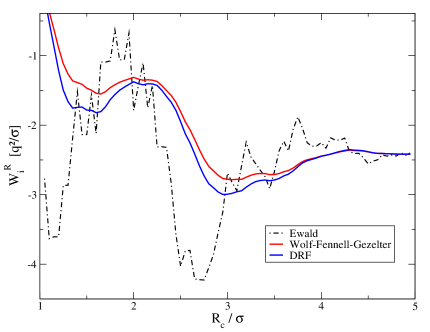
Figure 9: Evolution of the total virial with the cut-off radius. Molten ionic compound with stoichiometry 1:1. $\alpha=0.4~{}\sigma^{-1}$.

IV Convergence and optimization

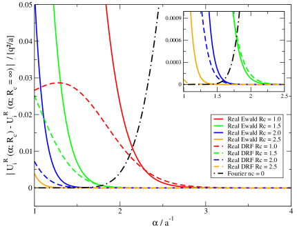
Figure 10: Deviation of the energy from its convergence value (Rc = $\infty$) as a function of $\alpha$ calculated for several cut-off radii. Comparison between Ewald summation and DRF method. $\Delta U^{F}_{i}(\alpha;n_{c}=0)$ is shown as a black dotted-dashed line in both plots. NaCl perfect crystal.

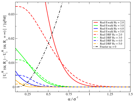
Figure 11: Deviation of the energy from its convergence value (Rc = $\infty$) as a function of $\alpha$ calculated for several cut-off radii. Comparison between Ewald summation and DRF method. $\Delta U^{F}_{i}(\alpha;n_{c}=0)$ is shown as a black dotted-dashed line in both plots. Molten ionic compound with stoichiometry 1:1.

In the previous sections we have shown analysis similar to those of Ref.Wolf et al., 1999; Fennell and Gezelter, 2006, which indicate that for sufficiently small $\alpha$, one can devise effective pairwise potentials that allow to approximate the Coulomb sum, Eq. (1), at low computational cost. Furthermore, we have shown that the damped reaction field method converges at least as good as WM and WFG methods, but has a sounder physical interpretation.

However, our theoretical analysis reveals that DRF, as well as WM and WFG, are in fact plausible approximations for the real space Ewald sum, Eq. (3), whether one opts to neglect the reciprocal space sum (Eq. (4)) or not. This is a very relevant issue which has apparently not been considered previously. It suggest one could perform the full Ewald summation, accounting both for the real space and Fourier contributions (whether in the standard implementation or in the particle mesh approaches Toukmaji and Board, 1996), but using DRF in order to accelerate the convergence of the real space term. This would allow to perform the Coulomb sum with arbitrary precision, but decreasing the cost of the real space sum.

In order to study this question in more depth, we introduce a measure of the truncation error performed in the real space sum as follows:

$$\Delta U^{\rm R}_{i}(\alpha;R_{c})=\ \mid U^{\rm R}_{i}(\alpha;R_{c})-U^{\rm R}_{i}(\alpha;R_{c}=\infty)\mid$$ (37)

A plot of the real space convergence error is shown in Fig.10 for the case of crystalline NaCl. Full lines indicate the error that results when Eq. (3) is evaluated by sum of plain $\mathrm{e}rfc(\alpha r)/r$ contributions, i.e., RSE, and dashed lines the case where it is evaluated using DRF. The figure clearly shows that, for reasonable choices of $R_{c}$, there is a range of small $\alpha$, where DRF exhibits much smaller convergence error than RSE. However, as $\alpha$ increases, the difference becomes smaller, and actually exhibits a crossover to a regime where the plain RSE seems to perform better.

At any rate, the convergence is always improved for large values of $\alpha$. However, one can not increase $\alpha$ arbitrarily, because then the Fourier contribution would become relevant. In order to optimize the choice of $\alpha$ for a given fixed $R_{c}$, the relevant issue is then what the error of neglecting the Fourier sum is.

In order to asses this, we now introduce a measure of the truncation error performed in the reciprocal space sum of Eq. (4). This error results from the neglect of contributions with reciprocal space vectors ${\bf k}=\frac{2\pi}{L}(n_{x},n_{y},n_{z})$ larger than a prescribed cutoff, $k_{c}$. Similarly to Eq. (37), we can therefore introduce a Fourier space truncation error as:

$$\Delta U^{F}_{i}(\alpha;n_{c})=\ \mid U^{F}_{i}(\alpha;n_{c})-U^{F}_{i}(\alpha;n_{c}=\infty)\mid\\$$ (38)

where $n_{c}$ defines a cubic cutoff for vectors whose integer components (absolute value) are larger than $n_{c}$.

Obviously, the pairwise effective potentials as estimated in WM and WFG, as well as in the zero dipole method of Ref.Fukuda et al. (2011), neglect the Fourier space contribution all together. This corresponds to assuming a Fourier space convergence error for zero cutoff, $n_{c}=0$.

Fig.10 displays together with $\Delta U^{\rm R}_{i}(\alpha;R_{c})$ the Fourier space convergence error $\Delta U^{\rm F}_{i}(\alpha;n_{c})$ for the special case where $n_{c}=0$.

Clearly, it is always possible to choose a value of $\alpha$ sufficiently small that $\Delta U^{\rm F}_{i}(\alpha;n_{c}=0)$ is negligible. However, the optimal choice of $\alpha$ is one where both $\Delta U^{\rm R}_{i}(\alpha;R_{c})$ and $\Delta U^{\rm F}_{i}(\alpha;n_{c})$ are of similar order. Obviously, it does not make much sense to achieve an exceptional convergence in the real space contribution, if this is at the cost of having a much larger reciprocal space error, because what matters is the overall convergence of the full Coulomb sum.

Unfortunately, Fig.10 seems to suggest that $\Delta U^{\rm F}_{i}(\alpha;n_{c}=0)$ cuts $\Delta U^{\rm R}_{i}(\alpha;R_{c})$ at a point where there is no significant advantage of the DRF method over the plain RSE summation. i.e., the point at which $\Delta U^{\rm F}_{i}(\alpha;n_{c}=0)$ is about the same order of magnitude of $\Delta U^{\rm R}_{i}(\alpha;R_{c})$ occurs where DRF and RSE perform similarly. This seems clearly visible, at least for the perfect NaCl crystal and three choices of $R_{c}/a=1,1.5$ and $2$.

The same conclusions may be drawn from Fig.11, which plots the convergence errors for the case of the molten salt. Here, the situation seems to be even less advantageous for DRF, since the region of $\alpha$ where it exhibits smaller error than the plain RSE is smaller. In fact, in this case $\Delta U^{\rm F}_{i}(\alpha;n_{c}=0)$ cuts the curves $\Delta U^{\rm R}_{i}(\alpha;R_{c})$ after the crossover where RSE converges better than DRF, for all but the smallest $R_{c}$ studied.

We now study the optimization of the Ewald sum by relaxing the constraint of pairwise schemes, i.e., by allowing for a finite reciprocal space cutoff. This is still a relevant issue, since the Ewald sum requires to share the computational cost between both the real and Fourier contributions.Kolafa and Perram (1992) An improvement in the convergence of the real space summation would allow to shift some of the cost of the reciprocal space sum to the real space term, making the former less expensive.

Fig.12-13 display $\Delta U^{\rm R}_{i}(\alpha;R_{c})$ as estimated from RSE and DRF, compared with $\Delta U^{\rm F}_{i}(\alpha;n_{c})$ for crystalline and molten NaCl, respectively. Notice that the errors are shown in logarithmic scale, with large negative values indicating small errors.

From inspection of $\Delta U^{\rm R}_{i}(\alpha;R_{c})$, it now becomes clear that one can identify two different regimes. Firstly, a reaction field regime corresponding to small values of the product $\alpha R_{c}$, where DRF produces smaller real space errors than the plain Ewald real space sum. Secondly, an Ewald regime, of large $\alpha R_{c}$, where it is actually the RSE summation which performs better than DRF, and presumably, better than whichever pairwise effective potential scheme.

Optimization of the Ewald sum requires to choose $R_{c}$, $\alpha$ and $n_{c}$ such that $\Delta U^{\rm R}_{i}(\alpha;R_{c})\approx\Delta U^{\rm F}_{i}(\alpha;n_{c})$. Thus, a mixed scheme using DRF and reciprocal space sums would be advantageous over the Ewald method if the condition above is met at a value of $\alpha$ where the convergence error of DRF is smaller than that of RSE. Unfortunately, our plots seem to indicate that this is not usually the case. Only for the special choice of $n_{c}=0$, i.e., for complete neglect of the reciprocal space sum, we find that an optimized DRF yields errors similar to the optimized RSE.

Notice that the conclusions drawn above are restricted to bulk systems. Additional care must be taken for inhomogeneous systems, where the charge distribution may exhibit large or even diverging correlations of long wavelength. The charge structure factor $\rho({\bf k})$ in Eq. (4) then becomes very large for small ${\bf k}$, and the reciprocal space sum is significant even for small $\alpha$. Empirically, this has been observed by Takahashi et al., who studied the liquid-vapor interface of SPCE/E water and noticed the convergence of Wolf’s method could only be achieved for cutoffs as large as 20 molecular diameters.Takahashi et al. (2011) Such a poor convergence indicates very long range, small wave-vector interactions across the interface. These are best dealt by transferring some of the real space computational burden to the reciprocal space sum, which precisely is devised to ensure fast convergence of small wave-vector contributions. Theoretically, it has been shown that properly taking into account a large scale inhomogeneity requires to account for the net dipole moment of the system in the direction perpendicular to the interface. Such contribution, which is significant and independent of the choice of $\alpha$, corresponds to a zero wave-vector term of the reciprocal space sum and cannot possibly be accounted for with a real space finite cutoff.de Leeuw et al. (1980); Hautman et al. (1989); Spohr (1997); Yeh and Berkowitz (1999)

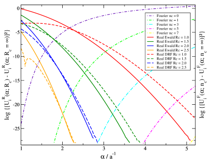
Figure 12: Quadratic deviation of the real and the reciprocal part of the energy from its convergence value (infinite Rc or nc) as a function of $\alpha$ calculated for several cut-off radii. Comparison between Ewald summation and DRF method. NaCl perfect crystal.

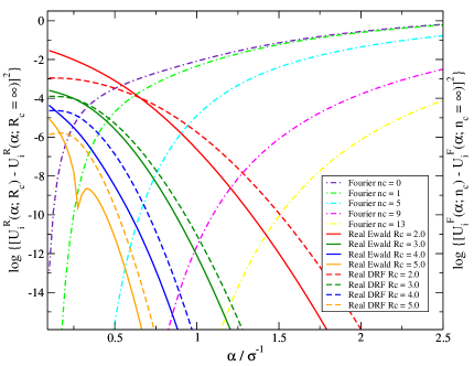
Figure 13: Quadratic deviation of the real and the reciprocal part of the energy from its convergence value (infinite Rc or nc) as a function of $\alpha$ calculated for several cut-off radii. Comparison between Ewald summation and DRF method. Molten ionic compound with stoichiometry 1:1.

V Conclusions

In this work we have considered a number of recent methodologies which allow to approximate the electrostatic energy of charged systems by means of effective pairwise potentials.Wolf et al. (1999); Fennell and Gezelter (2006); Fukuda et al. (2011)

Our theoretical study reveals that these methods may be actually considered as approximations to the real space Ewald sum only, Eq. (3), rather than to the sought Coulomb sum, Eq. (1). This is an important matter, because it means that the pairwise effective potentials cannot possibly account for the long range electrostatic response of charged systems. Particularly, such methods cannot account ab-initio for the surface term of the Coulomb energy, which is recovered in the full Ewald sum as the $k=0$ limit to the reciprocal space term.de Leeuw et al. (1980); Ballenegger (2014)

For cases where the damping parameter $\alpha$ is small enough, however, all terms besides the $k=0$ contribution to the reciprocal space sum are negligible and the Ewald self term, Eq. (5) is then a very good approximation for the Fourier space contribution, Eq. (4).

In such cases, our numerical study shows that pairwise effective potentials produce indeed a better convergence of the real space Ewald sum than the Ewald pair potential itself. In practice, this may be achieved by introducing a shifted,Wolf et al. (1999) or a shifted force,Fennell and Gezelter (2006) potential. However, our theoretical analysis shows that the correct electrostatic treatment may achieve both the potential and force shift by means of a generalization of the reaction field method,Fukuda et al. (2011) which damps the Coulomb potential via an $\mathrm{e}rfc(\alpha r)$ function. This damped reaction field method, used as an approximation to the real space Ewald sum smoothly transforms from a pure reaction field to an effective Ewald sum, by tuning the damping parameter $\alpha$.

We have studied the performance of the modified Coulomb sums in a particularly difficult case of an ionic crystal and its melt. This provides a stringent test of all methods and thus allows to draw more general conclusions. Our results show that the new damped reaction field method, which has a much more clear electrostatic significance, is also the method which provides better convergence of the energy and the virial for both the crystal and the melt.

A close inspection of the convergence errors allows to identify two different regimes. Firstly, a reaction field regime, corresponds to small $\alpha R_{c}$, where effective pair wise methods such as the damped reaction field method converge better than the bare $\mathrm{e}rfc(\alpha r)/r$ potential. Secondly, an Ewald regime, corresponding to large $\alpha R_{c}$, where the bare Ewald potential actually converges better than all effective pair wise methods studied. Our numerical study shows that the crossover from the reaction field to the Ewald regime occurs precisely for those values of $\alpha$ where the reciprocal space sum has an error about the same size as the real space sum. Since this equality is the condition for optimization of the Coulomb sum,Kolafa and Perram (1992) the implication is that for an optimized calculation of the electrostatic energy the Ewald sum method is not improved by effective pair wise methods. Such methods do remain useful and produce improved convergence of the Ewald sum in those cases where high accuracy calculations, or optimization of the Coulomb sum are not a concern. Alternatively, they might also be competitive in cases where the availability of parallel computing does not make competitive the calculation of the reciprocal space sum.