On the Per-Sample Capacity of
Nondispersive Optical Fibers

Abstract

The capacity of the channel defined by the stochastic nonlinear Schrödinger equation, which includes the effects of the Kerr nonlinearity and amplified spontaneous emission noise, is considered in the case of zero dispersion. In the absence of dispersion, this channel behaves as a collection of parallel per-sample channels. The conditional probability density function of the nonlinear per-sample channels is derived using both a sum-product and a Fokker-Planck differential equation approach. It is shown that, for a fixed noise power, the per-sample capacity grows unboundedly with input signal. The channel can be partitioned into amplitude and phase subchannels, and it is shown that the contribution to the total capacity of the phase channel declines for large input powers. It is found that a two-dimensional distribution with a half-Gaussian profile on the amplitude and uniform phase provides a lower bound for the zero-dispersion optical fiber channel, which is simple and asymptotically capacity-achieving at high signal-to-noise ratios (SNRs). A lower bound on the capacity is also derived in the medium-SNR region. The exact capacity subject to peak and average power constraints is numerically quantified using dense multiple ring modulation formats. The differential model underlying the zero-dispersion channel is reduced to an algebraic model, which is more tractable for digital communication studies, and in particular it provides a relation between the zero-dispersion optical channel and a $2\times 2$ multiple-input multiple-output Rician fading channel. It appears that the structure of the capacity-achieving input distribution resembles that of the Rician fading channel, i.e., it is discrete in amplitude with a finite number of mass points, while continuous and uniform in phase.

I Introduction

Although the capacity of many classical communication channels has been established, determining the capacity of fiber-optic channels has remained an open and challenging problem. The capacity of the optical fiber channel is difficult to evaluate because signal propagation in optical fibers is governed by the stochastic nonlinear Schrödinger (NLS) equation, which causes signal and noise to interact in a complicated way. This paper evaluates the capacity for models of the optical fiber channel in the case of zero dispersion.

The deterministic NLS equation is a partial differential equation in space and time exhibiting linear dispersion and a cubic nonlinearity, giving rise to a deterministic model of pulse propagation in optical fibers in the absence of noise. When distributed additive white noise is incorporated, a waveform communication channel is defined. This channel has an input-output map that is not explicit and instantaneous, but involves the evolution of the transmitted signal along the space dimension.

The exact capacity of the optical fiber with dispersion and nonlinearity is not yet known. Results so far are limited to lower bounds on the capacity in certain regimes of propagation or under some conditions. Some of these works include modeling the nonlinearity by multiplicative noise in the wavelength-division multiplexing (WDM) case [1], assuming a Gaussian distribution for the output signal when nonlinearity is weak [2], perturbing the nonlinearity parameter [3], approaching capacity via multiple-ring modulation formats [4], or specializing to the important case of zero dispersion [2, 5], which is the focus of this paper.

When dispersion is zero, pulse propagation is governed only by the Kerr nonlinearity and amplified spontaneous emission (ASE) noise. This eliminates the time-dependence of the stochastic NLS, reducing it to a nonlinear ordinary differential equation (ODE) as a function only of distance $z$. For a certain suboptimal receiver, as assumed later in the paper, transmission is then sample-wise and the channel can be viewed as a collection of parallel independent sub-channels, with noise interacting with the nonlinearity in the same channel, but not with neighboring channels located at other times. The problem becomes easier to analyze since, instead of describing the evolution of a random waveform and its entropy rate, we merely need to look at the evolution of a random variable and its entropy, which can be described by a single conditional probability density function (PDF).

In [2], Tang estimated the capacity in the dispersion-free case using Pinsker’s formula, based on the channel input-output correlation functions. Tang’s results show that capacity, ${\mathcal{C}}$, increases with input power power, ${\mathcal{P}}$, reaching a peak at a certain optimal input power, and then asymptotically vanishes as ${\mathcal{P}}\rightarrow\infty$. Estimates of the capacity in the general case [1, 3, 6, 4] also exhibit this behavior. However, the results of [2] can be viewed only as a lower bound on the capacity (even when the nonlinearity is weak), since the second-order statistics used in Pinsker’s formula do not capture the entire conditional PDF, which, of course, is required for the computation of ${\mathcal{C}}$.

The conditional probability density function (of the channel output given the channel input) for the dispersion-free optical fiber has been derived in [5] and [7]. In [5], the authors used the Martin-Siggia-Rose formalism in quantum mechanics to find a closed-form expression for the conditional joint PDF of the received signal amplitude and phase. Although they did not explicitly compute the capacity, they showed that the capacity asymptotically goes to infinity for large signal-to-noise ratios (SNRs).

With the exception of a few papers (e.g., [1, 2, 3, 5, 6, 4]), optical fiber communication is largely unstudied from the information theory point of view. Most previous papers on the capacity of optical fibers have focused on the dispersive channel directly from its description given by the stochastic nonlinear Schrödinger equation. This direct approach has had limited success, due to the complexity of the underlying channel model and its limited mathematical understanding. The stochastic nonlinear Schrödinger equation with dispersion parameter set to zero, on the other hand, leads to a model which is the basic building block of the dispersive optical fiber channel. It is therefore of fundamental interest to first study the zero-dispersion case. In this paper, we pursue such a bottom-up approach. Below, we highlight some of the contributions of this paper.

In Sec. III-A, we provide a simple derivation of the conditional PDF of the channel output given the channel input. Our approach is based on discretizing the fiber into a cascade of a large number of small fiber segments, which leads to a recursive computation of the PDF. An alternative perspective, using a stochastic calculus approach, is provided in Appendix A.

In Sec. III-B, we show that the probabilistic channel model in optical fibers can be understood in terms of the sum-product algorithm, or as a path integration. Such path integrals underlie the Martin-Siggia-Rose formalism, which was employed in [5].

In Sec. IV, for the first time to the best of our knowledge, the capacity of the dispersionless fiber is numerically evaluated as a function of the signal-to-noise ratio, for fixed noise spectral densities. The results re-affirm the conclusion of [5] that the channel capacity (when measured in bits per symbol) grows unbounded, at a fixed noise level, with increasing signal power.

In Sec. V, a decomposition is established between the amplitude and phase channels. The decoupling has the property that the input phase does not statistically excite the output amplitude. Using this amplitude and phase decomposition, the asymptotic result of [5] is then easily proved.

Also in Sec. V, a simplified model is derived for the dispersion-free optical channel. Simplification is achieved by reducing the differential model underlying the zero-dispersion channel to an algebraic model, which is more tractable for digital communication studies. Instead of a stochastic differential equation, the channel’s input/output relation is explicitly expressed as a simple 2$\times$2 MIMO system, similar to MIMO wireless multi-antenna models.

In Sec. VI we return to the amplitude/phase decomposition, and show that the phase channel exhibits a phase transition property: for very small or high signal power levels, the phase channel conveys little information, and the maximum information rate is achieved at a finite optimal power. This phase transition property partitions the ${\mathcal{P}}$-$\sigma^{2}$ plane into four regions which behave in different ways. This partitioning also enables us to find practically significant bounds on the capacity in some of these regions.

In [8] it was shown that for a simple intensity-modulation direct-detection (IM/DD) optical channel, a half-Gaussian distribution is asymptotically capacity-achieving at high SNRs. An important conclusion of Sec. VI is that, a two-dimensional distribution with a half-Gaussian profile on the amplitude and uniform phase provides an excellent global lower bound for the zero-dispersion optical fiber channel, which is simple and asymptotically capacity-achieving in a certain high SNR regime where ${\mathcal{P}}\rightarrow\infty$ and noise power is fixed.

In Sec. VII, we show that the channel capacity is indeed a two-dimensional function of the signal and noise powers and, unlike classical linear channels, is not completely captured by the signal-to-noise ratio.

In Sec. VIII, we address the relationship between the spectral efficiency in bits/s/Hz and capacity in bits/symbol. For many practical pulse shapes, even though the capacity (in bits/symbol) grows without bound (in agreement with [5]), spectral broadening resulting from the fiber nonlinearity sends the spectral efficiency (in bits/s/Hz) to zero (in agreement with the estimates of [2]). This result also agrees with the spectral-efficiency estimates of [1, 3, 6, 4] for fiber channels with nonzero dispersion.

In Sec. IX, the optical fiber at zero dispersion is related to the Rician fading channel in wireless communication. Although we do not provide a formal proof, numerical simulations indicate that the optimal capacity-achieving input distribution for the dispersion-free optical fiber appears to be discrete in amplitude and uniform in phase.

II Notation

The notation in this paper is mostly consistent with [9]. We use upper-case letters to denote scalar random variables taking values on the real line $\mathbb{R}$ or in the complex plane $\mathbb{C}$, and lower-case letters for their realizations. Random vectors are denoted with bold-face capital letters while their realizations are denoted by boldface lower-case letters. All deterministic quantities are treated as realizations of random variables. In order to avoid confusion with scalar random variables, we represent constant matrices with sans serif font, such as $\sf{K}$, $\sf{M}$, $\sf{P}$, and important scalars with calligraphic font such as power $\mathcal{P}$, bandwidth $\mathcal{W}$, capacity $\mathcal{C}$, rate $\mathcal{R}$. We reserve lower case Greek and Roman letters for special scalars. Real and complex normal random variables are shown as $\mathcal{N}_{\mathbb{R}}$ and $\mathcal{N}_{\mathbb{C}}$. We use the shorthand notation $\{\textbf{Z}_{k}\}\sim\textrm{IID}$ $\mathcal{N}_{\mathbb{R}}(0,\sigma^{2})$ to denote a sequence of real, independent, identically-distributed zero-mean Gaussian random variables with variance $\sigma^{2}$.

III Channel Model

Let $Q(z,t)$ be the complex envelope of the propagating electric field as a function of distance $z$ and time $t$, the latter measured with respect to a reference frame copropagating with the signal. Signal evolution in optical fibers with zero dispersion and distributed Raman amplification is modeled by the stochastic nonlinear ODE (see, e.g., [4, Eqn. (1) with $\beta_{2}=0$])

$$\frac{\partial Q(z,t)}{\partial z} = j\gamma Q(z,t)|Q(z,t)|^{2}+V(z,t),$$

$$Q(0,t) = Q_{0}(t),\quad 0\leq z\leq{\mathcal{L}}.$$ (1)

Here ${\mathcal{L}}$ is the length of the fiber, $V(z,t)$ is a zero-mean Gaussian process uncorrelated in space and time, i.e., with

$$\mathsf{E}[V(z,t)V^{*}(z^{\prime},t^{\prime})]=\sigma_{0}^{2}\delta(z-z^{\prime},t-t^{\prime}),$$

and $Q_{0}(t)$ is the complex envelope of the electric field applied at the fiber input. Finally, $\gamma$ is the Kerr nonlinearity parameter and $\sigma_{0}^{2}$ is the noise power spectral density. Following [4], we assume the fiber parameters given in Table I, with $\sigma_{0}^{2}=n_{\rm sp}h\nu\alpha=5.906\times 10^{-21}~{}{\rm W/(km}\cdot{\rm Hz)}$. The transmitted power is denoted as

$$P_{Q_{0}}=\frac{1}{{\mathcal{T}}}\int_{0}^{{\mathcal{T}}}|Q_{0}(t)|^{2}dt.$$

The transmitter will be constrained so that $\mathsf{E}P_{Q_{0}}={\mathcal{P}}_{0}$.

The stochastic differential equation (1) is interpreted in the Itô sense via its equivalent integral representation [10]. Note that in (1) the white noise $V(z,t)$ is added to the spatial derivative of the signal, as opposed to the signal itself, and has units of ${\rm W}^{1/2}/{\rm km}$. Note further that (1) contains no loss parameter, since losses are assumed to be perfectly compensated for by Raman amplification [11]. The time variable $t$ appears in (1) essentially as a parameter. Some limitations of the zero-dispersion model (1) are discussed in Section VIII.

TABLE I: Fiber Parameters

$n_{\rm sp}$ 1 spontaneous emission factor $h$ $6.626\times 10^{-34}{\rm J}\cdot{\rm s}$ Planck’s constant $\nu$ 193.55 THz center frequency $\alpha$ $0.046~{}{\rm km}^{-1}$ fiber loss (0.2 dB/km) $\gamma$ $1.27~{}{\rm W}^{-1}{\rm km}^{-1}$ nonlinearity parameter $B$ 125 GHz maximum bandwidth

Suppose the communication channel (1), i.e., the waveform channel from $Q(0,t)$ to $Q({\mathcal{L}},t)$, is used in the time interval $[0,{\mathcal{T}}]$ for some fixed ${\mathcal{T}}$ and that the input waveform $Q_{0}(t)$ is approximately bandlimited to ${\mathcal{W}}_{0}$ Hz. It is well known that, if ${\mathcal{W}}_{0}{\mathcal{T}}\gg 1$, the set of possible transmitted pulses spans a complex finite-dimensional signal space (called here the input space) with approximately $2{\mathcal{W}}_{0}{\mathcal{T}}$ dimensions (complex degrees of freedom). Since the channel is dispersionless, the pulse duration remains constant during propagation; however, as discussed in Sec. VIII, the pulse bandwidth may continuously grow because of the nonlinearity. We denote by ${\mathcal{W}}_{\mathcal{L}}$ the bandwidth of the waveform received at the output of the fiber. The received waveform is an element of a signal space (called here the output space) of dimension $2{\mathcal{W}}_{\mathcal{L}}{\mathcal{T}}\geq 2{\mathcal{W}}_{0}{\mathcal{T}}$. In other words, the dimension of the signal space grows while the signal is propagated.

We consider a model in which noise throughout the fiber is bandlimited to ${\mathcal{W}}_{{\mathcal{L}}}$ using in-line channel filters. Therefore, throughout the fiber, the noise lies in the output space. Both the input waveform and the output waveform can be represented by samples taken $1/2{\mathcal{W}}_{{\mathcal{L}}}$ seconds apart. At the fiber input, where the signal is constrained to lie in the input space, information can be encoded in samples corresponding to the input signal degrees of freedom (called the principal samples). All other samples are interpolated as appropriate linear combinations of the principal samples. These samples, though not innovative, carry correlation information, much like parity-checks in a linear code, that are potentially useful for optimal detection.

In this paper, however, we consider a suboptimal receiver that ignores the additional samples, and bases its decision only on the principal samples. The resulting channel is consequently a set of parallel independent scalar channels (called per-sample channels) defined via

$$\frac{\partial Q(z)}{\partial z} = j\gamma Q(z)|Q(z)|^{2}+V(z),$$

$$\mathsf{E}[V(z)V^{*}(z^{\prime})] = \sigma^{2}\delta(z-z^{\prime}),\qquad\mathsf{E}|Q_{0}|^{2}\leq{\mathcal{P}},$$ (2)

where $\sigma^{2}=2{\mathcal{W}}_{{\mathcal{L}}}\sigma_{0}^{2}$, $Q_{0}\in\mathbb{C}$ is the channel input sample value, and ${\mathcal{P}}$ is the per-sample power. The output of the channel is $Q({\mathcal{L}})\in\mathbb{C}$.

III-A A Simple Recursive Derivation of the Conditional PDF

The differential model in the form given by (2) is not directly suitable for an information-theoretic analysis. Instead, we require an explicit input-output probabilistic model, i.e., the conditional probability density function of the channel output given the channel input. The conditional PDF of $Q({\mathcal{L}})$ given $Q(0)$ was derived in [7] and [5]. Although the direct calculation of moments of the received signal, or equivalently the moment generating function as in [7], leads to an expression for the PDF, it does not provide enough insight into the statistical nature of the channel. The approach of [5] relies on the Martin-Siggia-Rose formalism in quantum mechanics and expresses the PDF as a path integral. Below we derive the PDF in a simple way, by breaking the fiber into a cascade of a large number of small segments, and recursively compute the PDF. With this approach, we are able to illustrate some important properties of the statistical channel model.

In order to describe the statistics of the per-sample channels in (2), we look at the fiber as a cascade of a large number $n\rightarrow\infty$ of pieces of discrete fiber segments by discretizing the equation (2). The recursive stochastic difference equation giving the input-output relation of the $k^{\textrm{th}}$ incremental channel is given by

$$Q_{k+1}=Q_{k}+j\epsilon\gamma|Q_{k}|^{2}+\sqrt{\epsilon}V_{k},\quad{0\leq k\leq n-1},$$ (3)

in which $\epsilon={\mathcal{L}}/n$, and the discrete noise $V_{i}\sim\mathcal{N}_{\mathbb{C}}(0,\sigma^{2})$ has been scaled by the square root of the step size, i.e., multiplied by $1/\sqrt{\epsilon}$. Note that from (3) the cascade of incremental fiber segments forms a discrete-time continuous-state Markov chain

$$Q_{0}\rightarrow Q_{1}\rightarrow\cdots\rightarrow Q_{n-1}.$$ (4)

Given $Q_{0}$, the signal entropy is increased by a tiny, signal-dependent, amount in each of these incremental channels. In fact, the conditional entropy increases more for transmitted signals with higher amplitude than those with smaller amplitude. In a sphere-packing picture, “noise balls” surrounding a transmitted symbol increase in volume as the symbol amplitude increases, and indeed are not perfectly spherical.

Each of the incremental channels, though still nonlinear with respect to the input signal, is conditionally Gaussian with PDF

$$f_{Q_{k+1}|Q_{k}}(q_{k+1}|q_{k}) = \frac{1}{\pi\sigma^{2}\epsilon}$$ (5)

$$\exp\left(-\frac{\left|q_{k+1}-q_{k}-j\epsilon\gamma q_{k}|q_{k}|^{2}\right|^{2}}{\epsilon\sigma^{2}}\right).$$

Using the Markov property (4), the probability density function for the cascade of two consecutive incremental channels is given by the Chapman-Kolmogorov equation

$$f_{Q_{k+2}|Q_{k}}(q_{k+2}|q_{k})=$$

$$\int\limits_{\mathbb{C}}f_{Q_{k+2}|Q_{k+1}}(q_{k+2}|q_{k+1})f_{Q_{k+1}|Q_{k}}(q_{k+1}|q_{k})dq_{k+1}.$$ (6)

Repeated application of (6) gives the overall conditional PDF

$$f_{Q_{n}|Q_{0}}(q_{n}|q_{0})=\int\limits_{\mathbb{C}}\ldots\int\limits_{\mathbb{C}}\frac{1}{(\pi\sigma^{2}\epsilon)^{n}}$$ (7)

$${}\prod_{k=0}^{n-1}{}\>\exp\left(-\frac{\left|q_{k+1}-q_{k}-j\epsilon\gamma|q_{k}|^{2}q_{k}\right|^{2}}{\epsilon\sigma^{2}}\right)\prod_{k=1}^{n-1}dq_{k}$$

$$= \frac{1}{\pi\sigma^{2}\epsilon}\int\limits_{\mathbb{C}}\ldots\int\limits_{\mathbb{C}}\exp\left\{-\frac{\epsilon}{\sigma^{2}}\left[\sum\limits_{k=0}^{n-1}\left|\frac{q_{k+1}-q_{k}}{\epsilon}-j\gamma|q_{k}|^{2}q_{k}\right|^{2}\right]\right\}$$ (8)

$$\times\frac{dq_{n-1}}{\pi\epsilon\sigma^{2}}\frac{dq_{n-2}}{\pi\epsilon\sigma^{2}}\cdots\frac{dq_{1}}{\pi\epsilon\sigma^{2}},$$

where $q_{k}=r_{k}\exp(j\phi_{k})$ and integrations are performed over the entire complex plane.

We proceed to solve multiple integrals (8). First a change of variables is introduced to make the exponent quadratic in $q_{k}$. The integrating factor for the noiseless equation (2) serves as the new variable

$$p_{k}=q_{k}\exp\left(-j\epsilon\gamma\sum\limits_{m=0}^{k-1}\left|q_{m}\right|^{2}\right)\quad k=1,\ldots,n-1.$$ (9)

Plugging (9) into (8), each term in the exponent, except the first and last terms, is

$$\epsilon\left|\frac{q_{k+1}-q_{k}}{\epsilon}-j\gamma|q_{k}|^{2}q_{k}\right|^{2}\\ =\epsilon\biggl{|}\frac{p_{k+1}\exp(j\epsilon\gamma|p_{k}|^{2})-p_{k}}{\epsilon}-j\gamma|p_{k}|^{2}p_{k}\biggr{|}^{2}\\ =\epsilon\left|\frac{p_{k+1}-p_{k}}{\epsilon}\right|^{2}+O(\epsilon^{2}),$$

where we have assumed $(p_{k+1}-p_{k})/\epsilon$ is bounded. It follows that each middle term in the exponent of (7) is simplified to $\epsilon\left|\frac{p_{k+1}-p_{k}}{\epsilon}\right|^{2}$, which is correct up to first order in $\epsilon$.

The treatment of the boundary terms is different and in particular they lead to new expressions. The first term is treated as above to give

$$\epsilon\biggl{|}\frac{p_{1}\exp(j\epsilon\gamma|q_{0}|^{2})-q_{0}}{\epsilon}-j\gamma|q_{0}|^{2}q_{0}\biggr{|}^{2}=\epsilon\left|\frac{p_{1}-q_{0}}{\epsilon}\right|^{2}+O(\epsilon^{2}),$$

while the last term reads

$$\epsilon\biggl{|}\frac{q_{n}\exp\left(-j\gamma\epsilon\sum\limits_{k=0}^{n-1}|p_{k}|^{2}\right)-p_{n-1}}{\epsilon}\biggr{|}^{2}+Q(\epsilon^{2}).$$

As can be seen, the end point is now interpreted as $q_{n}\exp(-j\epsilon\gamma\sum\limits_{k=0}^{n-1}|p_{k}|^{2})$ which has a variable phase. In order to consistently convert all correlated integrals to Gaussian type integrals, one can assume that the received phase

$$\theta_{n}=\phi_{n}-\epsilon\gamma\sum\limits_{k=0}^{n-1}|p_{k}|^{2},$$ (10)

is constant, and then integrate over $0\leq\theta_{n}<2\pi$. For fixed $\theta_{n}$, the resulting integrand is an exponential with a complex quadratic polynomial in the exponent, and boundary terms $r_{0}\exp j\phi_{0}$ and $r_{n}\exp j\theta_{n}$. However phase constraint (10) implies that for each value of $\theta_{n}$, integration is performed under the constraint $\epsilon\gamma\sum\limits_{k=0}^{n-1}|p_{k}|^{2}=\phi_{n}-\theta_{n}$.

To enforce constraint (10), the function under the integration is multiplied by the delta function representing that constraint, giving

$$\delta\left(\phi_{n}-\theta_{n}-\epsilon\gamma\sum\limits_{k=0}^{n-1}|p_{k}|^{2}\right)$$

$$= \sum\limits_{m=-\infty}^{\infty}\delta\left(\phi_{n}-\theta_{n}-\epsilon\gamma\sum\limits_{k=0}^{n-1}|p_{k}|^{2}+2m\pi\right)$$

$$= \frac{1}{2\pi}\sum\limits_{m=-\infty}^{\infty}\exp\left[jm\left(\phi_{n}-\theta_{n}-\epsilon\gamma\sum\limits_{k=0}^{n-1}|p_{k}|^{2}\right)\right].$$

where we have used phase periodicity and expanded the train of impulse functions as a complex Fourier series.

Summarizing, the conditional PDF now reads

$$f_{Q_{n}|Q_{0}}(q_{n}|q_{0})=\frac{1}{2\pi}\sum\limits_{m=-\infty}^{\infty}e^{jm\phi_{n}}\int\limits_{\theta_{n}=0}^{2\pi}e^{-jm\theta_{n}}\ \\ \frac{1}{\pi\sigma^{2}\epsilon}\int\limits_{\mathbb{C}}\ldots\int\limits_{\mathbb{C}}\exp\left\{-\epsilon\sum\limits_{k=0}^{n-1}\left[\frac{1}{\sigma^{2}}\left|\frac{p_{k+1}-p_{k}}{\epsilon}\right|^{2}+j\gamma m|p_{k}|^{2}\right]\right\}\\ \times\frac{dp_{n-1}}{\pi\epsilon\sigma^{2}}\frac{dp_{n-2}}{\pi\epsilon\sigma^{2}}\cdots\frac{dp_{1}}{\pi\epsilon\sigma^{2}},$$ (11)

where we assumed $p_{0}=q_{0}$ and $p_{n}=r_{n}\exp j\theta_{n}$, and used the fact that the Jacobian of the transformation (9) is unity, since it represents a lower triangular matrix with unit magnitude on its diagonal elements.

The integrals in (11) are complex Gaussian and can be solved directly. We proceed to calculate

$$T_{m}(r_{n})=\int\limits_{0}^{2\pi}d\theta_{n}e^{-jm\theta_{n}}\int\limits_{\mathbb{C}}\ldots\int\limits_{\mathbb{C}}\frac{dp_{n-1}}{\pi\epsilon\sigma^{2}}\frac{dp_{n-2}}{\pi\epsilon\sigma^{2}}\cdots\frac{dp_{1}}{\pi\epsilon\sigma^{2}}\times$$

$$\frac{1}{\pi\sigma^{2}\epsilon}\exp\left\{-\epsilon\sum\limits_{k=0}^{n-1}\left[\frac{1}{\sigma^{2}}\left|\frac{p_{k+1}-p_{k}}{\epsilon}\right|^{2}+j\gamma m|p_{k}|^{2}\right]\right\}.$$ (12)

This is done by first integrating over phases, starting from the very last term $\theta_{n}$ where only one variable is involved. It can be shown that (III-A) simplifies to

$$T_{m}(r_{n})=\left(\frac{2}{\epsilon\sigma^{2}}\right)^{n}e^{-jm(\theta_{0}+\gamma\epsilon r_{0}^{2})}\exp\left(-\frac{r_{n}^{2}+r_{0}^{2}}{\epsilon\sigma^{2}}\right)$$ (13)

$$\int\limits_{r_{n-1}}^{\infty}\cdots\int\limits_{r_{1}}^{\infty}dr_{n-1}\cdots dr_{1}$$

$$\prod\limits_{k=1}^{n-1}r_{k}\exp\left\{-\frac{2+jm\gamma\epsilon^{2}\sigma^{2}}{\epsilon\sigma^{2}}r_{k}^{2}\right\}I_{m}\left(\frac{2r_{k}r_{k+1}}{\epsilon\sigma^{2}}\right)$$

$$\times I_{m}\left(\frac{2r_{1}r_{0}}{\epsilon\sigma^{2}}\right),$$ (14)

where $I_{m}$ denotes the $m^{th}$ order modified Bessel function of the first kind, and where we have used (62) from Appendix B.

Integrals (14) involve products of Bessel functions and can be computed iteratively with the help of identity (63) in Appendix B. We have

$$T_{m}(r_{2}) = \frac{2}{\epsilon\sigma^{2}(2+jm\gamma\epsilon^{2}\sigma^{2})}e^{-jm(\theta_{0}+\gamma r_{0}^{2}\epsilon)}$$

$$\times \exp\left\{-\frac{1}{\epsilon\sigma^{2}}\left(\frac{1+jm\gamma\epsilon^{2}\sigma^{2}}{2+jm\gamma\epsilon^{2}\sigma^{2}}\right)(r_{0}^{2}+r_{2}^{2})\right\}$$

$$\times I_{m}\left(\frac{2r_{0}r_{2}}{\epsilon\sigma^{2}(2+jm\gamma\epsilon^{2}\sigma^{2})}\right).$$

As the calculations for $T_{m}(r_{2})$ and identity (63) suggest, $T_{m}(r_{n})$ keeps its structure for $n\geq 3$, and can be parametrized in the form

$$T_{m}(r_{n}) = 2b_{n}(m)e^{-jm(\theta_{0}+\gamma r_{0}^{2}n\epsilon)}\exp\left\{-a_{n}(m)(r_{0}^{2}+r_{n}^{2})\right\}$$ (15)

$$\times I_{m}\left(2b_{n}(m)r_{0}r_{n}\right),$$

where $a_{n}(m)$ and $b_{n}(m)$ are parameters to be determined. It can be shown that $T_{m}(r_{n})$ satisfies

$$T_{m}(r_{n+1})=\int\limits_{r_{n}=0}^{\infty}K(r_{n},r_{n+1})T_{m}(r_{n})dr_{n},$$ (16)

where kernel $K(r_{n+1},r_{n})$ is

$$K(r_{n+1},r_{n})=\frac{2}{\epsilon\sigma^{2}}r_{n}$$

$$\exp\left\{-\frac{1}{\epsilon\sigma^{2}}\left[r_{n+1}^{2}+(1+jm\gamma\epsilon^{2}\sigma^{2})r_{n}^{2}\right]\right\}I_{m}(\frac{2r_{n}r_{n+1}}{\epsilon\sigma^{2}}).$$

Substituting (15) into (16) and comparing exponents on both sides, recursive equations are obtained for $a_{n}(m)$ and $b_{n}(m)$, namely,

$$b_{n+1} = \frac{b_{n}}{\epsilon\sigma^{2}[a_{n}+\frac{1+jm\gamma\epsilon^{2}\sigma^{2}}{\epsilon\sigma^{2}}]},$$

$$a_{n+1} = \frac{1}{\epsilon\sigma^{2}}-\frac{1}{(\epsilon\sigma^{2})^{2}[a_{n}+\frac{1+jm\gamma\epsilon^{2}\sigma^{2}}{\epsilon\sigma^{2}}]}$$

$$= a_{n}-\frac{jm\gamma\epsilon^{2}\sigma^{2}}{\epsilon\sigma^{2}}-\frac{b_{n}^{2}}{[a_{n}+\frac{1+jm\gamma\epsilon^{2}\sigma^{2}}{\epsilon\sigma^{2}}]},$$

with

$$a_{2}=\frac{1+jm\gamma\epsilon^{2}\sigma^{2}}{\epsilon\sigma^{2}(1+jm\gamma\epsilon^{2}\sigma^{2})},\qquad b_{2}=\frac{1}{\epsilon\sigma^{2}(2+jm\gamma\epsilon^{2}\sigma^{2})}.$$

Solving these equations, we obtain expressions for $a(m)$ and $b(m)$ in the limit as $n\rightarrow\infty$ ($n\epsilon={\mathcal{L}}$):

$$a(m) = \lim_{\begin{subarray}{c}n\epsilon={\mathcal{L}}\\ n\rightarrow\infty\end{subarray}}a_{n}(m)=\frac{\sqrt{jm\gamma}}{\sigma}\coth\sqrt{jm\gamma\sigma^{2}}{\mathcal{L}},$$

$$b(m) = \lim_{\begin{subarray}{c}n\epsilon={\mathcal{L}}\\ n\rightarrow\infty\end{subarray}}b_{n}(m)=\frac{\sqrt{jm\gamma}}{\sigma}\frac{1}{\sinh\sqrt{jm\gamma\sigma^{2}}{\mathcal{L}}}.$$ (17)

Finally, using (III-A) we obtain the conditional PDF of $Q$ in the zero-dispersion model (2)

$$f(r,\phi|r_{0},\phi_{0}) = \frac{f_{R|R_{0}}(r|r_{0})}{2\pi}$$ (18)

$$\>+\frac{1}{\pi}\sum_{m=1}^{\infty}\Re\left(C_{m}(r)e^{jm(\phi-\phi_{0}-\gamma r_{0}^{2}{\mathcal{L}})}\right),$$

where $f_{R|R_{0}}(r|r_{0})$ is the probability density of the amplitude of the received signal

$$f_{R|R_{0}}(r|r_{0})=\frac{2r}{\sigma^{2}{\mathcal{L}}}\exp(-\frac{r^{2}+r_{0}^{2}}{\sigma^{2}{\mathcal{L}}})I_{0}(\frac{2rr_{0}}{\sigma^{2}{\mathcal{L}}}),$$ (19)

and where the Fourier coefficient $C_{m}(r)$ is given by

$$C_{m}(r)=rb(m)\exp\left[-a(m)\left(r^{2}+r_{0}^{2}\right)\right]I_{m}(2b(m)r_{0}r).$$

Remark 1.

Note that $f(r,\phi|r_{0},\phi_{0})$ is symmetric with respect to the phase $\phi$. We rely on this property in Sec. IV to simplify the optimization problem in the capacity question.

Remark 2.

One can verify that the conditional PDF of the amplitude of the received field given the amplitude of the transmitted signal (19) is in fact the conditional PDF for the intensity-modulated direct-detection (IM/DD) channel

$$R_{k}=\left|Q_{0}^{k}+Z_{k}\right|\quad k=0,1,\ldots,$$ (20)

where $Z_{k}\sim\mathcal{N}_{\mathbb{C}}(0,\sigma^{2}{\mathcal{L}})$. It is easy to see that the conditional PDF depends only on $R_{0}=|Q_{0}|$, as in (19).

The conditional PDF (18) defines a communication channel having the complex plane as the input alphabet, for which the information capacity ${\mathcal{C}}$ is defined as

$${\mathcal{C}}({\mathcal{P}},\sigma^{2}{\mathcal{L}},\gamma) = \max\limits_{f(r_{0},\phi_{0})\in{\mathcal{F}}}\quad I(R,\Phi;R_{0},\Phi_{0})$$ (21)

$$\textnormal{subject to}\quad ER_{0}^{2}\leq{\mathcal{P}},$$

where

$$I(R,\Phi;R_{0},\Phi_{0}) {=} \iiiint f(r_{0},\phi_{0})f(r,\phi|r_{0},\phi_{0})$$

$$\cdot\>\log\frac{f(r,\phi|r_{0},\phi_{0})}{f(r,\phi)}dr_{0}d\phi_{0}drd\phi,$$

and where ${\mathcal{F}}$ is the space of probability densities, and $f(r,\phi)=\iint f(r,\phi|r_{0},\phi_{0})f(r_{0},\phi_{0})dr_{0}d\phi_{0}$.

The per-sample capacity (21) can be related to the capacity of the waveform dispersion-free optical channel. It can be argued that a uniform power allocation is optimal for principal samples. The capacity of the entire ensemble of the principal per-sample channels is

$$2{\mathcal{W}}_{0}{\mathcal{T}}{\mathcal{C}}\left(\frac{{\mathcal{P}}_{0}}{2{\mathcal{W}}_{0}{\mathcal{T}}},\frac{2\sigma_{0}^{2}{\mathcal{L}}{\mathcal{W}}_{{\mathcal{L}}}}{2{\mathcal{W}}_{0}{\mathcal{T}}},\gamma\right)\quad\textnormal{bits per channel use},$$

which, as discussed before, is a lower bound on the capacity of the zero-dispersion waveform channel (1). Therefore in this paper we only estimate the per-sample capacity of (2).

The following theorem is a simple way to establish the results of [5].

Theorem 1.

Let $\rho={\mathcal{P}}/\sigma^{2}{\mathcal{L}}$ be the signal-to-noise ratio. Then ${\mathcal{C}}\geq\frac{1}{2}\log\rho-\frac{1}{2}$ and in particular $\lim\limits_{\rho\rightarrow\infty}{\mathcal{C}}(\rho)=\infty$.

Proof:

Using the chain rule for mutual information

$$I(R,\Phi;R_{0},\Phi_{0}) = I(R;R_{0},\Phi_{0})+I(\Phi;R_{0},\Phi_{0}|R)$$

$$\geq I(R;R_{0},\Phi_{0})=I(R;R_{0}).$$

As mentioned in Remark 2, $I(R;R_{0})$ is the mutual information function for the intensity-modulated direct-detection (IM/DD) channel for which the lower bound $\frac{1}{2}\log\rho-\frac{1}{2}$ is already known [7]. It therefore follows that ${\mathcal{C}}\geq\frac{1}{2}\log\rho-\frac{1}{2}$. ∎

Put in other words, Theorem 1 simply says that the amount of information which can be sent over the complex channel (2) is no less than what can be transmitted and received by the amplitude alone. From (19), the communication channel from $R_{0}$ to $R$ does not depend on the nonlinearity parameter $\gamma$, is independent of input phase and supports an unbounded information rate when increasing power indefinitely. Since the capacity of (2) was discussed to be a lower bound to the capacity of (1), we conclude that the capacity of the zero dispersion optical fiber (1) also goes to infinity with SNR.

III-B Sum-product probability flow in zero-dispersion fibers

The recursive computation of the PDF in the previous section was algebraic and still not a suitable way to visualize signal statistics. In this section, we show that the structure of the probability flow in zero-dispersion fibers is given by the sum-product algorithm or a path integral. Such path integration underlies the Martin-Siggia-Rose formalism in quantum field theory (QFT), which was directly used in [5]. This connects the results of the previous section to [5].

Computation of the conditional PDF as explained in the previous section was a marginalization process. In our example, the Markov property (4) made it possible to perform marginalization, since the conditional PDF factors as a product of certain normalized functions. This observation allows us to apply the sum-product algorithm known already in coding theory. As a matter of fact, the reader can notice that (7) is a sum-product computation, with a slight difference that instead of multiple summation, we performed multiple integrations, which is indeed a continuous limit of the sum-product algorithm in the signal dimension. It might be, however, more insightful to restore the analysis and represent the technique in the discrete domain.

While discretizing the fiber in the distance dimension, we will also at the end of at each fiber segment quantize the signal $q_{k}$ into a large number of small bins in the complex plane

$$q_{k}\in\mathcal{S} = \{q_{n}^{m}=r_{n}\exp(j\phi_{m})|r_{n}=n(\delta r),\quad n=1,\ldots,N,\quad$$ (22)

$$\phi_{m}=m(\delta\phi),\quad m=0,1,\ldots,M-1\},$$

for small $\delta r$ and $\delta\phi$. This turns each incremental channel into a discrete memoryless channel (DMC) described by a transition matrix; moreover, the overall channel matrix is the product of all of these transition matrices. The probability of receiving $q_{k}^{l}=r_{k}\exp j\phi_{l}$ at $z={\mathcal{L}}$ given the $q_{i}^{j}=r_{i}\exp j\phi_{j}$ is transmitted at $z=0$, is the sum over the probability of all possible transitions (paths) from $q_{i}^{j}$ to $q_{k}^{l}$. This is graphically illustrated in Fig. 1 as a trellis. Nodes of the trellis are quantized points in the complex plane and edges have weights corresponding to transition probabilities (5).

Figure 1: Graphical computation of the probability density function $f(r,\phi|r_{0},\phi_{0})$. The probability of receiving $r_{n}\exp\phi_{m}$ given transmission of $r_{k}\exp\phi_{l}$ is the sum over the probability of each possible path between start and end points shown schematically in the figure. The probability of each path is the product of of the transition probabilities of all edges forming that path, computable from (5).

It follows that the essence of the probabilistic model in optical fibers is a propagator ${\sf{A}}(\delta r,\delta\phi,\epsilon)$, independent of spatial index $k$, which for the case of (2) can be described by a single functional matrix

$$[{\sf{A}}(\delta r,\delta\phi,\epsilon)]_{i,j}=\frac{|q_{n}^{m}|\delta r\delta\phi}{\pi\sigma^{2}\epsilon}\exp\left(-\frac{\left|q_{n}^{m}-q_{k}^{l}-j\epsilon\gamma q_{k}^{l}|q_{k}^{l}|^{2}\right|^{2}}{\epsilon\sigma^{2}}\right),$$

where $i=(k-1)M+l$ and $j=(n-1)M+m$. The probabilities of $\{q_{n}^{m}\}_{n,m=0}^{N,M}$ are then recursively updated as

$$\textbf{p}(k+1)={\sf{A}}(\delta r,\delta\phi,\epsilon)\textbf{p}(k),$$

where p is the vector of the probabilities of $\{q_{n}^{m}\}_{n,m=0}^{N,M}$. By diagonalizing the propagator ${\sf{A}}={\sf{U}}{\sf{\Lambda}}{\sf{U}}^{-1}$, the overall conditional distribution is $\textbf{p}(n)={\sf{U}}{\sf{\Lambda}}^{n}{\sf{U}}^{-1}$, which is a function of eigenvalues and eigenvectors of the propagator.

In the language of the statistical mechanics, the limit of the expression (8) when $n\rightarrow\infty$ is a path integral and is represented as

$$f_{Q|Q_{0}}(q|q_{0})=$$

$$\int_{r_{0}e^{j\phi_{0}}}^{re^{j\phi}}\exp\left(-\int_{0}^{z}\frac{\left|\frac{\partial q}{\partial z^{\prime}}-j\gamma|q(z^{\prime})|^{2}q(z^{\prime})\right|^{2}}{\sigma^{2}}dz^{\prime}\right)\mathfrak{D}q,$$ (23)

where the expression is understood as in [12]. Equation (III-B) is just a symbolic representation of (8) and follows from the definition of the path integral [12], [13].

The computation of path integrals whose exponent can be made quadratic in $q$ and $\partial q/\partial z$ is standard in quantum mechanics and, in the case of (III-B), this computation has been done in [5] to find the conditional PDF. Indeed path integral (III-B) is an immediate consequence of the Martin-Siggia-Rose formalism, a more generic framework in quantum mechanics dealing with stochastic dynamical systems [5]. To compute (III-B), roughly speaking, one needs to sum over the input-output paths giving the largest contributions, i.e., the path corresponding to minimizers of the integral exponent in (III-B). This classical path is given by the Euler-Lagrange equations, with all other paths considered as a perturbation around this classical path, serving as a normalization constant in the PDF.

It is interesting to see the effect of the change in variables (9) in the sum-product algorithm. One can verify that the equation (2) when noise is zero has the solution

$$q(z)=q_{0}\exp(j\gamma|q_{0}|^{2}z).$$ (24)

In other words, while the signal is propagated down the noiseless fiber, it remains on a circle in the complex plane with radius $|q_{0}|$ and rotates counterclockwise with phase velocity $\gamma|q_{0}|^{2}$ rad/m. We call this solution the deterministic path, which is a helix twisted around the fiber. With the change of variable (9), the accumulated phase from the beginning of the fiber to an arbitrary distance $z$ is subtracted from the (nonlinear) phase of the signal, to compensate for the signal rotation. The deterministic path is then a straight line, rather than a twisted helix. In this view, (24) gives rise to nonlinear phase compensation at the receiver, often used in optical communications.

When using (9), the trellis in Fig. 1 is transformed to a new trellis. Since the change of variable (9) has memory of the form $\exp\left(-j\epsilon\gamma\sum\limits_{m=0}^{k-1}\left|q_{m}\right|^{2}\right)$, it causes a transformation from paths to points

$$\mathbb{P}:(q_{0},q_{1}^{m_{1}},q_{2}^{m_{2}},\cdots,q_{k}^{m_{k}})\mapsto p_{k}^{l}.$$

In general $q_{n}^{m}$ at stage $k$ of the old trellis is mapped to a number of points at stage $k+1$ in the new trellis, depending on the total number of paths from $q_{0}$ to $q_{n}^{m}$. These points lie on a circle and correspond to rotations of constellations in the old trellis. The structure of the $p$-trellis, in the limits $\delta r,\delta\phi\rightarrow 0$, is same as Fig. 1 except that instead of a single terminal point at the end of the diagram, there is a circle of radius $|q_{k}^{l}|$. The transformed trellis is shown in Fig. 2.

Figure 2: Transformation of the q-trellis (the trellis in Fig. 1) under the transformation (9). The result is called the p-trellis.

The expression (7) is then the sum over the probability of all transition paths starting with $q_{0}=q_{i}^{j}$ and ending in any of the resulting terminal points. The overall sum can be decomposed into a number of subgroups, with each subgroup a sum-product from $r_{i}\exp j\phi_{j}$ to one of the output terminal points $r_{k}\exp j\theta_{l}$, for some $l$ as in (22). The total sum is then obviously sum over all these sub-sum-products corresponding to different phase levels

$$P[r_{k}\exp j\phi_{l}|r_{i}\exp j\phi_{j}]\\ =\sum\limits_{\textnormal{all possible }\theta_{l}}\mathbb{\textnormal{SP}}(q_{0}=q_{i}^{j}\rightarrow q_{k}^{l}=r_{k}\exp j\theta_{l}),$$

where $\mathbb{\textnormal{SP}}(q_{0}=q_{i}^{j}\rightarrow q_{k}^{l}=r_{k}\exp j\theta_{l})$ is a sum-product from $q_{i}^{j}$ to $q_{k}^{l}$. In terms of Fig. 2, this is a sum-product from $q_{0}$ to one of the points on the terminal circle. Note that, however, each sum-product from $r_{i}\exp j\phi_{j}$ to $r_{k}\exp j\theta_{l}$ is a constrained sum-product, i.e., instead of all possible paths between these two points, the summation in (III-A) is performed over only feasible paths consistent with (10). This is accomplished by multiplying the edge-weights by an indicator function representing (10), and then summing over all possible paths between $r_{i}\exp j\phi_{j}$ to $r_{k}\exp j\theta_{l}$. The indicator function is later expanded in terms of Fourier series to make analytical computations possible.

IV Numerical Evaluation of the Capacity

In this section we numerically evaluate the per-sample capacity of the communication channel (2) to observe the general trend of the capacity as a function of the input average power. In particular, we are interested in observing the effect of the signal-dependent noise in the absence of dispersion. The spectral efficiency of the dispersive optical channel as a function of the input power is known to have a peak [1]. The peak is often attributed to the fact that increasing the signal power will increase the noise power as well (which is signal-dependent). The same type of behavior was observed in [2] for the nondispersive channel as well. In this section, we numerically observe that with no dispersion, although the channel is still nonlinear, the signal-dependent noise is not strong enough to suppress the capacity to zero.

We consider a 5000 km optical fiber operating at zero average dispersion and using distributed Raman amplification [11]. Among several sources of noise, ASE noise is assumed to be the dominant stochastic impairment, which can be modeled as additive white Gaussian noise. All other nominal simulation parameters are given in Table. I [4, 14].

We sample the conditional PDF (18) in a high resolution grid in the complex plane with $N$ rings and $M$ symbols on each ring. The values of $N$ and $M$, or the size of bins, depend on the noise standard deviation and are chosen so that in each noise standard deviation there are sufficiently many bins so that the conditional PDF of the channel is normalized over the entire partition. This is very similar to the multiple ring modulation format, an idea well-known in the context of AWGN channels and recently employed in optical communication in [4].

The accumulated noise level in the optical fiber, albeit signal dependent, is still much smaller than the noise level in typical AWGN channels. Thus compared to the AWGN channels, more resolution is needed to numerically approach the capacity of optical channels via this technique. In addition, it is known that in a dispersive channel, dispersion and nonlinearity to some extent cancel out each some of the detrimental effects of the other, leading to a balanced propagation. In the absence of dispersion such balance does not exist anymore, and the channel exhibits stronger nonlinear properties. This makes it more difficult to numerically evaluate the capacity of the dispersionless channel.

Estimates of the capacity are found and compared using two methods: the Blahut-Arimoto algorithm with power constraint [15] and a logarithmic barrier interior-point method [16]. From the phase symmetry of the channel matrix, a capacity-achieving input distribution will have uniform phase distribution. In both algorithms, we enforce this constraint to make the problem effectively a one dimensional optimization program, which considerably stabilizes and speeds up the underlying numerical optimization.

Note that the Blahut-Arimoto algorithm in its original form was developed for linear inequality constraints, and cannot be directly used to approximate the capacity in a region where ${\mathcal{C}}$ is decreasing with ${\mathcal{P}}$. One might modify the original Blahut-Arimoto algorithm to take into account the equality constraints as well. However since in our numerical simulations capacity is never found to be constant when increasing power, the inequality power constraint is always active at the optimal solution and no such modification is required. Because for small SNRs capacity follows Shannon’s limit for linear Gaussian channels, the Lagrange multiplier is started at a large value and is iterated down to zero at the optimum, with increasing resolution.

The results of the numerical calculation of the capacity are shown in Figs. 3-5. Fig. 3

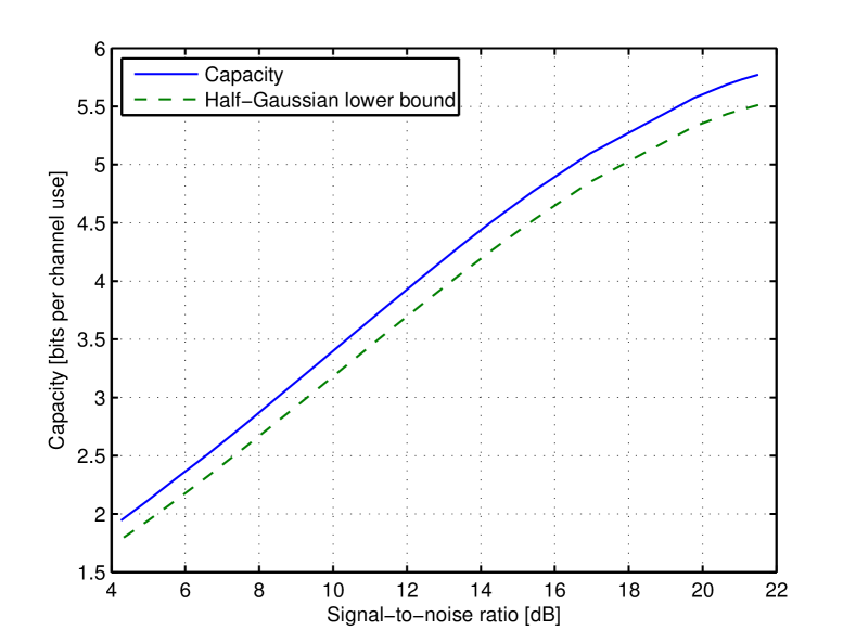
Figure 3: Capacity as a function of SNR with peak power ${\mathcal{P}}_{0}=10$mW and noise spectral density $10^{-1}\mu$W/GHz. The end of the graph occurs at about 20% of the peak power.

shows the per-sample capacity ${\mathcal{C}}$ of channel (2) as a function of input average signal power ${\mathcal{P}}$ for noise spectral density $10^{-1}~{}\mu$ W/GHz. We can see that the channel capacity increases indefinitely with the average input power. Moreover, as evident in Fig. 3, in the high power regime the capacity growth is linear on a logarithmic scale. To simulate at increased power levels, a prohibitive number of symbols is required.

Motivated by previous work [2, 5], we searched for peaks in the capacity curve for different set of fiber parameters. Simulations were performed for a wide range of parameters to operate at low and high SNRs. No peak was found within our computational ability of finding capacity at high SNRs.

Although there is no peak in the capacity curve, the phase channel $\Phi_{0}\mapsto(R,\Phi)$ was found to always having a global maximum in its ${\mathcal{C}}-{\mathcal{P}}$ plot. Intuitively this behavior is a consequence of the observation that the phase of the received field is uniform and independent of the transmitted signal, if very low or high energy signals are sent through the channel. For a fixed noise variance, when signal power level ${\mathcal{P}}$ is small, phase supports little information because the linear phase noise dominates and is uniformly distributed in $[0,2\pi]$. On the other hand when ${\mathcal{P}}$ is large, the nonlinear phase noise takes over the whole interval [0,$2\pi$] and the phase sub-channel is unable to carry data. This effect is illustrated in Fig. 4.

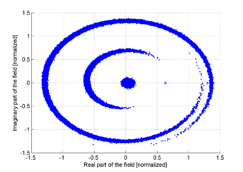
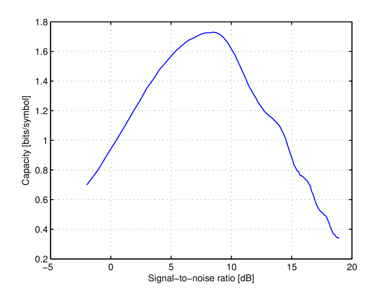
Figure 4: (a) Simulation of the optical phase channel channel operating at zero-dispersion for 3 transmitted points. It can be seen that for signals with very low or high power, the phase of the received signal contains almost no information. (b) Capacity of the phase modulation dispersion-free optical channel as a function of SNR.

In Fig. 5 we have plotted the capacity and the mutual information that uncoded phase-shift keying modulation formats can achieve in the zero-dispersion optical fiber. Similar to the AWGN channel, binary signaling is suboptimal at low SNRs (e.g., $\textnormal{SNR}<0$). More symbols are required to get close to the capacity with increasing SNR.

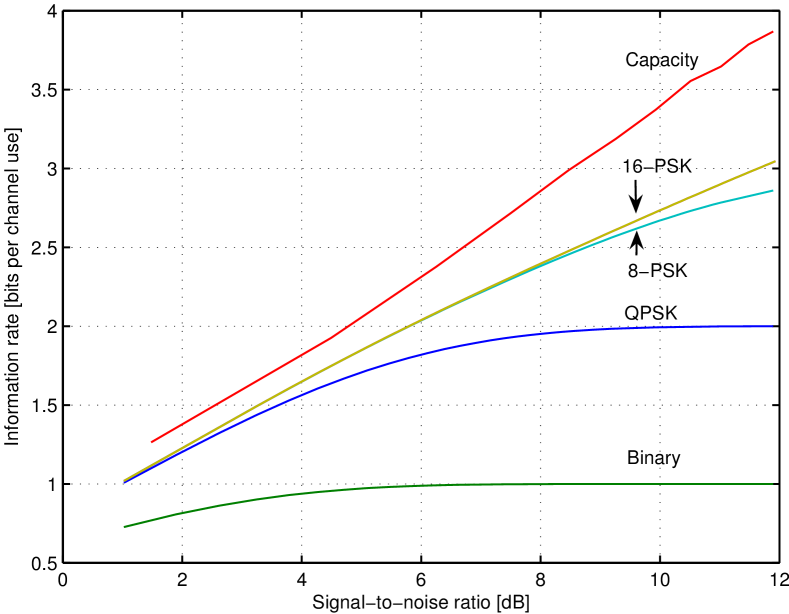
Figure 5: Achievable information rates in zero-dispersion optical fiber with M-PSK modulation formats

V An Algebraic Model

Although we used the PDF (18) to numerically find the capacity, it provides limited direct information-theoretic insights into the behavior of the channel. We therefore proceed with a more intuitive and simplified expression for the channel model. We reduce the differential model (2) to an algebraic model, which is more tractable for an information-theoretic analysis.

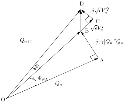
(a) (b)

Figure 6: (a) Vector diagram showing the signal evolution in the $n^{\textrm{th}}$ incremental piece of the fiber (b) Information streaming in the dispersion-free optical channel. Note that no information is transferred from $\Phi_{0}$ to $R$.

The vector diagram in Fig. 6(a) pictorially shows the evolution of the signal in the $n^{\textrm{th}}$ incremental piece of the fiber. The nonlinear term $j|Q|^{2}Q$ is orthogonal to the signal and, to the first order in $\epsilon$, does not change the amplitude. In other words, since in Fig. 6(a)

$$|\vec{OB}|=|\vec{OA}|+O(\epsilon^{2}),$$

the orthogonality of the nonlinearity to the signal implies that the nonlinear coefficient $\gamma$ is responsible only for an angular rotation; it does not contribute to random fluctuations across the radius. Therefore for the description of the amplitude channel we can set $\gamma=0$ without incurring any local or global error at the end of the fiber

$$|Q_{n+1}|=|\vec{OD}| = |\vec{OB}+\sqrt{\epsilon}V_{n}^{I}+j\sqrt{\epsilon}V_{n}^{Q}|$$ (25)

$$= |Q_{n}+\sqrt{\epsilon}V_{n}|+O(\epsilon^{2}),$$

where $V^{I}$ and $V^{Q}$ are in-phase and quadrature components of the noise, and we have used the fact that white noise preserves its properties under rotation. Similarly for the phase channel

$$\Phi_{n+1} = \Phi_{n}+\tan^{-1}j\gamma\epsilon|Q_{n}|^{2}+\tan^{-1}\frac{|\sqrt{\epsilon}V_{n}^{Q}|}{|R_{n}+\sqrt{\epsilon}V_{n}^{I}|}$$ (26)

$$= \Phi_{n}+\Phi_{L}+j\gamma\epsilon|Q_{n}|^{2}+O(\epsilon^{2}).$$

Hence from (25)-(26) it follows that

$$R(z)=|Q_{0}+W(z)|=|R_{0}+W(z)|,$$ (27)

$$\Phi(z)=\Phi_{L}(z)+\gamma\int_{0}^{z}|Q_{0}+W(z)|^{2},$$ (28)

where $W(z){=}\int_{0}^{z}V(\lambda)d\lambda$ is the Wiener process with $EW(z)W^{*}(z^{\prime}){=}\sigma^{2}\min(z,z^{\prime})$. The linear part of the phase $\Phi_{L}(z)$ from Fig. 6(a) is only a function of the amplitude $|\vec{OB}|$ and the noise $V_{n}$. As a result, setting $\gamma=0$ in (2) it is given by

$$\Phi_{L}(z)=\angle(Q_{0}+W(z)).$$ (29)

A byproduct of (27)-(29) is the compact solution of the nonhomogeneous stochastic ODE (2)

$$Q(z) = (Q_{0}+W(z))\exp(j\gamma\int\limits_{0}^{z}|Q_{0}+W(z^{\prime})|^{2}dz^{\prime}).$$ (30)

The first equation in the system (27)-(28) is decoupled from the second one and hence, neither deterministic amplitude nor its noisy perturbation depends on the Kerr nonlinearity constant $\gamma$. In particular, from (27) the probability density function of $R$ follows, as in (19). This is schematically shown in Fig. 6(b). Information is streamed from $R_{0}$ to $(R,\Phi)$, but $\Phi_{0}$ does not excite the output amplitude.

Amplitude and phase channels are defined by (27)-(29). Statistics can be directly computed from these equations and are generally signal-dependant Gaussian noises, and Gaussian squared (chi-squared) noise-noise beats. The original PDF can be rederived by calculating these statistics. To simplify the model, we replace the noise-noise beat terms with worst case Gaussian noises with the same mean and covariance matrix. In addition, we ignore the linear phase $\Phi_{L}$ compared to $\Phi_{\textnormal{NL}}$, which is stochastically valid for ${\mathcal{P}}\gg\sigma^{2}{\mathcal{L}}$. Though it is possible to calculate the statistics directly, it is generally easier to replace the Wiener process with its Karhunen-Loéve (KL) expansion in order to substitute the correlated sums with summations with uncorrelated terms and ease the following calculations. We are in accord of [17] concerning the use of Karhunen-Loéve expansion for such simplification. The KL expansion for the Wiener process reads [10]

$$W(z)=\sum\limits_{k=1}^{\infty}\sigma_{k}X_{k}\psi_{k}(z),\qquad 0\leq z\leq{\mathcal{L}},$$

where $\{X_{k}\}\sim\textrm{IID}$ $\mathcal{N}_{\mathbb{C}}(0,\sigma^{2}{\mathcal{L}})$ is a sequence of independent identically distributed zero-mean complex Gaussian random variables, and eigenvalues $\sigma_{k}$ and eigenfunctions $\psi_{k}(z)$ are defined as

$$\psi_{k}(z) = \sqrt{2}\sin\left(\frac{(2k-1)\pi}{2{\mathcal{L}}}z\right),\qquad 0\leq z\leq{\mathcal{L}},$$

$$\sigma_{k} = \frac{2}{(2k-1)\pi}.$$

At the end of the fiber $z={\mathcal{L}}$ we have, after some algebra,

$$R^{2} = |Q_{0}+Z_{1}|^{2}=R_{0}^{2}+2\Re{\{Q_{0}Z_{1}\}}+|Z_{1}|^{2},$$

$$\Phi \approx \Phi_{0}+\gamma{\mathcal{L}}\left(R_{0}^{2}+\frac{2}{\sqrt{3}}\Re{\{Q_{0}Z_{2}\}}+Z_{3}\right),$$ (31)

where $Z_{1}\sim\mathcal{N}_{\mathbb{C}}(0,\sigma^{2}{\mathcal{L}})$, $Z_{2}\sim\mathcal{N}_{\mathbb{C}}(0,\sigma^{2}{\mathcal{L}})$, $EZ_{1}Z_{2}^{*}=\frac{\sqrt{3}}{2}\sigma\sqrt{{\mathcal{L}}}$ and $Z_{3}=\sum_{k=0}^{\infty}\sigma_{k}^{2}|X_{k}|^{2}$ is a non-Gaussian random variable correlated with $Z_{1}$ and $Z_{2}$. In matrix notation

$$\textbf{Y}\simeq\textbf{X}+{\mathbb{H}}\textbf{Z}_{1}+\textbf{Z}_{2},\quad\textbf{Y}_{2}\>\textrm{mod}\>2\pi,$$ (32)

in which

$$\textbf{Y}=\left(\begin{array}[]{ll}R^{2}\\ \frac{\Phi}{\gamma{\mathcal{L}}}\end{array}\right),\ \textbf{X}=\left(\begin{array}[]{ll}R_{0}^{2}\\ \frac{\Phi_{0}}{\gamma{\mathcal{L}}}+R_{0}^{2}\end{array}\right),\mathbb{H}=\left(\begin{array}[]{ll}R_{0}&0\\ 0&R_{0}\end{array}\right),$$

and $\textbf{Z}_{1}\sim\mathcal{N}_{\mathbb{R}}\!\left(0,{\sf{P}}_{1}\right)$, while $\textbf{Z}_{2}$ is a non-zero mean random variable related to central chi-square random variables with $\mathsf{E}(\textbf{Z}_{2}-\mathsf{E}\textbf{Z}_{2})(\textbf{Z}_{2}-\mathsf{E}\textbf{Z}_{2})^{T}={\sf{P}}_{2}$. It can be shown that

$${\sf{P}}_{1}=\sigma^{2}{\mathcal{L}}\left(\begin{array}[]{ll}2&1\\ 1&\frac{2}{3}\end{array}\right),\quad{\sf{P}}_{2}=\sigma^{4}{\mathcal{L}}^{2}\left(\begin{array}[]{ll}1&\frac{1}{3}\\ \frac{1}{3}&\frac{1}{6}\end{array}\right),\quad\textbf{Z}_{1}\perp\textbf{Z}_{2}.$$

Gaussian random variables in model (32) can be further decoupled by performing the Cholesky factorization of the ${\sf{P}}_{1}=LL^{T}$ and processing ${\sf{L}}^{-1}\textbf{Y}$ as the output. Equations (V) can also be approximated as

$$R = |R_{0}+Z_{1}|,$$

$$\Phi \approx \Phi_{0}+\gamma{\mathcal{L}}|R_{0}+\frac{Z_{2}}{\sqrt{3}}|^{2},\qquad{\mathcal{P}}\gg\sigma^{2}{\mathcal{L}}.$$

From (32), nonlinearity introduces two important stochastic effects which are always absent in linear channels: signal-noise beat ${\sf{H}}\textbf{Z}_{1}$ and non-Gaussian noise-noise beat $\textbf{Z}_{2}$. In our problem, signal-noise beat is a simple signal-dependent noise in the form of the product of a Gaussian random variable with amplitude of the signal and stands for the amplification of the noise with signal during the propagation in the fiber. Noise-noise beat is related to chi-square random variables, which is independent of the signal, orthogonal to signal-noise beat and represents the gradual interaction of the Gaussian noise with itself through the nonlinearity.

VI Bounds on the Capacity – Performance of the Half-Gaussian Distribution

The algebraic model given in the equation (32) is a $2\times 2$ MIMO conditionally Gaussian channel model. It is very closely related to the Rician fading channel model, except that the term which comes directly from the signal at the output of (32) is the square of the signal, rather than the signal itself. However it still does not seem amenable to a closed form expression for the capacity.

For a simple intensity-modulated direct-detection channel (20), it is known that half-Gaussian distribution for the input amplitude (i.e., a Gaussian distribution truncated and normalized to nonnegative arguments) comes close to the capacity [8, 9]. Motivated by this, in this section we evaluate the mutual information that the half-Gaussian distribution $Q^{*}$ can achieve for the zero-dispersion optical channel, there $Q^{*}$ corresponds to the density function

$$f_{R_{0}.\Phi_{0}}(r_{0},\phi_{0})=\begin{cases}\frac{2}{2\pi\sqrt{2\pi{\mathcal{P}}}}\exp(-\frac{r_{0}^{2}}{2{\mathcal{P}}})&\text{if }r_{0}\geq 0,\\ 0&\text{if }r_{0}<0.\end{cases}$$

We show that, interestingly, a distribution with a truncated Gaussian profile on the amplitude and uniform phase provides an excellent global lower bound for the zero-dispersion optical fiber, and is asymptotically capacity-achieving in a high SNR region where ${\mathcal{P}}\gg\max\{\frac{6\pi^{2}}{\gamma^{2}\sigma^{2}{\mathcal{L}}^{3}},\sigma^{2}{\mathcal{L}}\}$. Note that the power of $Q^{*}$ is $\tilde{{\mathcal{P}}}=(1-\frac{2}{\pi}){\mathcal{P}}=0.36{\mathcal{P}}$.

Although the algebraic model (32) is much more tractable than (2) or the PDF (18), estimating the resulting output entropy for $Q^{*}$ is still complicated, though $f_{\textbf{Y}_{1},\textbf{Y}_{2}}(\textbf{y}_{1},\textbf{y}_{2})$ can be computed explicitly. In the case of a simple optical intensity channel, the data processing inequality for relative entropies was used in [9] to bound output entropy in terms of input entropy, by transferring the difficulty to the input side. This technique however is not immediately implementable for the two-dimensional problem here. We use several observations based on the algebraic model to evaluate the mutual information for the distribution $Q^{*}$.

Let $f_{\textbf{Y}_{2}|\textbf{X}_{2},{\mathbb{H}}}(\textbf{y}_{2}|\textbf{x}_{2},{\sf{H}})$ be the conditional probability density function of the phase channel in the simplified model (32). Replacing $\textbf{Z}_{2}$ with a worst-case Gaussian random variable with the same covariance matrix for the purpose of the lower bound, we have

$$f_{\textbf{Y}_{2}|\textbf{X}_{2},{\mathbb{H}}}(\textbf{y}_{2}|\textbf{x}_{2},{\sf{H}})=\sum\limits_{k=-\infty}^{\infty}\frac{1}{\sqrt{2\pi\sigma_{\textbf{Y}_{2}}^{2}}}\exp{-\frac{(\textbf{y}_{2}+2k\pi-\textbf{x}_{2})^{2}}{2\sigma_{\textbf{Y}_{2}}^{2}}}.$$

where $\sigma_{\textbf{Y}_{2}}^{2}$ is the variance of $\textbf{Y}_{2}$, and the summation is a result of $\textnormal{mod }2\pi$ reduction. Pictorially $f_{\textbf{Y}_{2}|\textbf{X}_{2},{\mathbb{H}}}(\textbf{y}_{2}|\textbf{x}_{2},{\sf{H}})$ is the summation of shifted Gaussians separated by distance $2\pi$. However if $\frac{2}{3}\sigma^{2}{\mathcal{L}}\left(\gamma{\mathcal{L}}\right)^{2}{\mathcal{P}}\ll(2\pi)^{2}$ all Gaussians are localized in the intervals $[-\frac{(k-1)\pi}{\gamma{\mathcal{L}}},\frac{(k+1)\pi}{\gamma{\mathcal{L}}}]$ centered approximately at the mean nonlinear phase noise and only one Gaussian is present in the interval of interest. In this region we would be able to find a lower bound by ignoring phase wraparounds. Conversely, if $\frac{2}{3}\sigma^{2}{\mathcal{L}}\left(\gamma{\mathcal{L}}\right)^{2}{\mathcal{P}}\gg(2\pi)^{2}$ all Gaussians look globally flat and from the symmetry of pairwise terms around the middle term, conditional phase tends to be uniformly distributed in $[\frac{-(k-1)\pi}{\gamma{\mathcal{L}}},\frac{(k-1)\pi}{\gamma{\mathcal{L}}}]$. In this case, we would be able to lower bound capacity by treating phase noise as a uniform random variable independent of the channel input. We make these intuitive statements precise in the next two subsections.

We also observe that in the zero-dispersion channel, it follows from phase symmetry that the capacity-achieving input distribution is uniform in phase, and thus the search for the optimal input distribution should be really done only over one-dimensional distributions. When applying the input distribution $Q^{*}$ to the original PDF (18), the sophisticated dependency on $\phi$ terms disappears since input phase is assumed to be uniform. We therefore use the exact original PDF (18) to find the output entropy, while conditional entropy is computed from the algebraic model (32). Offset term $\log|\det{\sf{J}}|$, with ${\sf{J}}$ being the Jacobian of the transformation relating these two models, is added to account for the mismatch between these two models.

VI-A Capacity bounds in the high-power regime

In the the high power regime where $\gamma^{2}{\mathcal{P}}\sigma^{2}{\mathcal{L}}^{3}\gg 6\pi^{2}$, the signal-dependent phase noise takes over the entire phase interval $[0,2\pi]$ and we conclude that phase carries no information. It follows that in this regime the zero-dispersion model (2) is reduced to the optical intensity-modulated direct-detection channel (20). For the latter channel, a lower bound was derived in [8] under average power constraint which is asymptotically exact. In fact, applying distribution $Q^{*}$ to the amplitude PDF (19), it is easy to show that

$${\mathcal{C}}_{H}\geq\frac{1}{2}\log(\rho)-\frac{1}{2},$$

where ${\mathcal{C}}_{H}$ is the capacity in the high-power regime, and $\rho={\mathcal{\tilde{P}}}/\sigma^{2}{\mathcal{L}}$ is the signal-to-noise ratio. Moreover from the duality-based upper bound developed in [9]

$${\mathcal{C}}_{H}\leq\frac{1}{2}\log(\rho)-\frac{1}{2}+o_{{\mathcal{P}}}(1),$$

where $o_{{\mathcal{P}}}(1)\rightarrow 0$ when ${\mathcal{P}}\rightarrow\infty$. We conclude that the capacity of the zero-dispersion optical channel asymptotically, in the region ${\mathcal{P}}\gg\max\{\frac{6\pi^{2}}{\gamma^{2}\sigma^{2}{\mathcal{L}}^{3}},\sigma^{2}{\mathcal{L}}\}$, is

$$C\sim\frac{1}{2}\log(\rho)-\frac{1}{2}.$$

A distribution with a half-Gaussian profile for the amplitude and uniform phase is capacity achieving at such high powers.

VI-B Capacity lower bound in the medium-power regime

As mentioned before, in a power region where $\gamma^{2}{\mathcal{P}}\sigma^{2}{\mathcal{L}}^{3}\ll 6\pi^{2}$, the effect of the phase wraparounds is negligible and the phase channel qualitatively acts similar to the amplitude channel. The resulting model is then similar to two amplitude channels correlated with each other

$$\textbf{Y}=\textbf{X}+{\sf{H}}\textbf{Z}_{1}+\textbf{Z}_{2},$$ (33)

where now Y is extended over the entire real line. We proceed to bound the mutual information for the distribution $Q^{*}$ and model (33)

$$I(R,\Phi;R_{0},\Phi_{0})|_{Q^{*}} = I(R^{2},\Phi;R_{0}^{2},\Phi_{0})|_{Q^{*}}$$

$$= h(R^{2},\Phi)-h(R^{2},\Phi|R_{0}^{2},\Phi_{0})$$

$$= h(\textbf{Y})-h(\textbf{Y}|\textbf{X}).$$

It can be shown that $\textbf{Z}_{1}\perp\textbf{Z}_{2}$ and therefore at the end of the fiber $z={\mathcal{L}}$ we can write

$${\sf{P}} = \mathsf{E}[(\textbf{Y}-\mathsf{E}\textbf{Y})(\textbf{Y}-\mathsf{E}\textbf{Y})^{H}|\textbf{X}]$$

$$= \sigma^{2}{\mathcal{L}}R_{0}^{2}\left(\begin{array}[]{ll}2&1\\ 1&\frac{2}{3}\end{array}\right)+\sigma^{4}{\mathcal{L}}^{2}\left(\begin{array}[]{ll}1&\frac{1}{3}\\ \frac{1}{3}&\frac{1}{6}\end{array}\right),$$

and

$$\det{\sf{P}}=\frac{\sigma^{4}{\mathcal{L}}^{2}}{3}(R_{0}^{4}+R_{0}^{2}\sigma^{2}{\mathcal{L}}+\frac{1}{6}\sigma^{4}{\mathcal{L}}^{2}).$$

Therefore for the conditional output entropy

$$h(\textbf{Y}|\textbf{X}) = \log(\gamma{\mathcal{L}})+\mathsf{E}_{\textbf{X}}[h(\textbf{Y}|\textbf{X}=\textbf{x}_{0})]$$

$$\leq \log(\gamma{\mathcal{L}})+\mathsf{E}_{R_{0},\Phi_{0}}[\frac{1}{2}\log((2\pi e)^{2}\det{\sf{P}})]$$

$$= \log(\gamma{\mathcal{L}})+\log(2\pi e)+\frac{1}{2}\log(\frac{\sigma^{4}{\mathcal{L}}^{2}}{3})$$

$$+ \frac{1}{2}E_{R_{0}}[\log(R_{0}^{2}+\alpha_{1}\sigma^{2}{\mathcal{L}})(R_{0}^{2}+\alpha_{2}\sigma^{2}{\mathcal{L}})],$$ (36)

in which $\alpha_{1}=\frac{3+\sqrt{3}}{6}$ and $\alpha_{2}=\frac{3-\sqrt{3}}{6}$. Note that the entropy of the small extra non-Gaussian ASE-ASE noise term $\textbf{Z}_{2}$ was upper bounded in (VI-B) by its equivalent worst-case Gaussian. For the half-Gaussian distribution, with the help of [18] one can verify that

$$E_{R_{0}}[\frac{1}{2}\log(R_{0}^{2}+q^{2}\sigma^{2}{\mathcal{L}})] = \frac{1}{2}\log({\mathcal{P}})-\frac{1}{2}\log(2)-\frac{1}{2}\zeta$$ (37)

$${-}\>\frac{q^{2}\sigma^{2}{\mathcal{L}}}{2{\mathcal{P}}}H([1,1],[\frac{3}{2},2],\frac{q^{2}\sigma^{2}{\mathcal{L}}}{2{\mathcal{P}}})$$

$${+}\>\frac{\pi}{2}\textrm{Erfi}(q\sqrt{\frac{\sigma^{2}{\mathcal{L}}}{2{\mathcal{P}}}}),$$

where $\zeta{=}0.5772$ is the Euler constant, $q\in\mathbb{R}^{+}$, $\textrm{Erfi}(x)=-j\textrm{erf}(jx)$ is the imaginary error function [18]

$$\textrm{Erfi(x)}=\frac{1}{\sqrt{\pi}}(2x+\frac{2}{3}x^{3}+\frac{1}{5}x^{5}+\frac{1}{27}x^{7}+\ldots),\,|x|\ll 1,$$

and $H(\textbf{p},\textbf{q},x)$ is the Hyper-geometric function

$$H([1,1],[\frac{3}{2},2],x) = \sum_{k=0}^{\infty}c_{k}x^{k}=1+\frac{1}{3}x+\frac{4}{45}x^{2}$$

$${+}\>\frac{4}{105}x^{3}+\ldots$$

$$\frac{c_{k+1}}{c_{k}} = \frac{k+1}{(k+\frac{3}{2})(k+2)}.$$

From (36)-(37)

$$h(\textbf{Y}|\textbf{X}) \leq \log({\mathcal{P}}\sigma^{2}{\mathcal{L}})+\log(\gamma{\mathcal{L}})+\log(2\pi e)$$ (38)

$$-\frac{1}{2}\log(3)-\log(2)-\zeta+F(\frac{\sigma^{2}{\mathcal{L}}}{2{\mathcal{P}}},\alpha_{1})$$

$$+\>F(\frac{\sigma^{2}{\mathcal{L}}}{2{\mathcal{P}}},\alpha_{2}).$$

where

$$F(x,\alpha)=\frac{\pi}{2}\textnormal{Erfi}(\sqrt{\alpha^{2}x})-\alpha^{2}xH([1,1],[\frac{3}{2},2],\alpha^{2}x).$$

Output entropy $h(\textbf{Y})$ cannot be straightly computed similar to $h(\textbf{Y}|\textbf{X})$ from the algebraic model (33). As explained at the beginning of this section, we instead exploit the phase symmetry of (18) and compute $h(\textbf{Y})$ directly from the original accurate PDF (18). The output PDF is computed as

$$f_{R,\Phi}(r,\phi) = \frac{\exp\left(-\frac{r^{2}}{2{\mathcal{P}}+\sigma^{2}{\mathcal{L}}}\right)}{2\pi\sqrt{\pi(2{\mathcal{P}}+\sigma^{2}{\mathcal{L}})}}[1+\textrm{erf}(\sqrt{\frac{2{\mathcal{P}}}{\sigma^{2}{\mathcal{L}}(2{\mathcal{P}}+\sigma^{2}{\mathcal{L}})}}r)]$$ (39)

$$\approx \frac{2}{2\pi}\frac{\exp\left(-\frac{r^{2}}{2{\mathcal{P}}+\sigma^{2}{\mathcal{L}}}\right)}{\sqrt{\pi(2{\mathcal{P}}+\sigma^{2}{\mathcal{L}})}}\qquad r\geq 0,$$

where the asymptote of the Bessel function $I_{0}(x)\sim\frac{1}{\sqrt{2\pi x}}\exp{x}$ has been used for $|x|\gg 1$, and $\frac{r}{r_{0}}\approx 1$. Note that this means that with uniform input phase, from the point of view of input-output densities, the zero-dispersion channel acts like the intensity-modulated direct-detection channel.

From (39) and changing the variable $\tilde{R}=R^{2}$, $f_{R^{2},\Phi}(r^{2},\phi)$ is obtained, which consequently leads to

$$h(\textbf{Y}){=}\frac{3}{2}\log(\pi)+\log(2{\mathcal{P}}+\sigma^{2}{\mathcal{L}})-\frac{1}{2}\zeta+\frac{1}{2}.$$ (40)

Finally from (40) and (38), a lower bound to the capacity of the zero-dispersion channel in the medium-power range $\sigma^{2}{\mathcal{L}}{\ll}{\mathcal{P}}{\ll}\frac{6\pi^{2}}{\gamma^{2}\sigma^{2}{\mathcal{L}}^{3}}$ follows

$${\mathcal{C}}_{M} \geq \frac{1}{2}\log(\frac{{\mathcal{P}}}{\sigma^{2}{\mathcal{L}}})+\frac{1}{2}\log(\frac{3\pi}{\gamma^{2}{\mathcal{P}}\sigma^{2}{\mathcal{L}}^{3}})+\frac{\zeta-1}{2}$$ (41)

$${-}\>F(\frac{\sigma^{2}{\mathcal{L}}}{2{\mathcal{P}}},\alpha_{1})-F(\frac{\sigma^{2}{\mathcal{L}}}{2{\mathcal{P}}},\alpha_{2}),$$

where $\zeta\approx 0.5772$ is the Euler constant.

The first term in (41) is $\frac{1}{2}\log(\rho)$ and is attributed to the amplitude channel. The rest of the terms are the phase contributions to the lower bound. Note that the lower bound (41) depends not only on the ratio $\rho={\mathcal{P}}/\sigma^{2}{\mathcal{L}}$, but also on the product of the signal and noise powers. In the low-power regime where ${\mathcal{P}}\ll\sigma^{2}{\mathcal{L}}$ the linear phase cannot be ignored relative to the nonlinear phase noise.

VII Two-dimensionality of the capacity

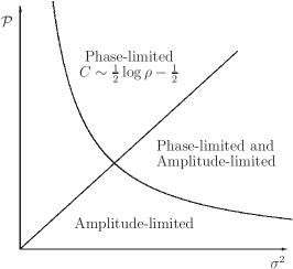
Figure 7: Fundamental transmission regimes in the ${\mathcal{P}}-\sigma^{2}$ plane. The line ${\mathcal{P}}=C_{1}\sigma^{2}$ marks the boundary between high and low SNR regimes, where the amplitude channel is approximately on, or approximately off. The curved boundary is of the form ${\mathcal{P}}=\frac{C_{2}}{\sigma^{2}}$ and separates two regions where the phase channel supports, or stops, to support information.

A distinguishing feature of the capacity of the system (2) is the two-dimensionality of the capacity as a function of both signal and noise powers. Unlike linear Gaussian channels, the dependency of the capacity of the nonlinear channels to signal and noise powers is not simply through the ratio $\rho={\mathcal{P}}/\sigma^{2}{\mathcal{L}}$. This is in sharp contrast to AWGN channels where capacity is completely captured by the signal-to-noise ratio.

For the IM/DD channel (20), it can be shown that although channel is still nonlinear in signal and noise, capacity is only a function of SNR. This basically follows from the scale-invariance property of the PDF (19) with respect to the noise power. The PDF of the whole channel (18) does not have such property. By scaling (2), if $(Q,V,\gamma)$ is a solution of (2), so is $(\lambda Q,\lambda V,\frac{\gamma}{\lambda^{2}})$. This implies that changing the Kerr coefficient, e.g., when $\lambda\rightarrow 0$, keeps the signal-to-noise ratio constant while capacity varies by $\gamma$. As a result, capacity is not completely captured by the SNR. It follows that when characterizing capacity as a function of SNR, one should make sure that within the working range of parameters, results are not affected by the choice of ${\mathcal{P}}$ and $\sigma^{2}$ for a fixed SNR.

VIII Spectral Considerations

Spectral efficiencies of the dispersion-free optical fiber have been studied in [2],[5]. In [2], the author used Pinsker’s formula to relate the spectral efficiency to input-output correlation functions. Such a result should be used with caution since second-order correlation functions do not capture the knowledge of the whole PDF, which is required for the computation of the capacity. In fact, Pinsker’s formula was originally formulated for (linear dispersive) Gaussian waveform channels. Therefore, the results of [2] can be viewed as a lower bound to the capacity, not ultimate achievable rates.

The asymptotic tail of the capacity was proved to be growing unboundedly in [5] by an asymptotic analysis. The authors then concluded that “a naive straightforward application of the Pinsker formula for evaluation of the capacity of a nonlinear channel as, for instance, in [2], can lead to wrong conclusions regarding the asymptotic behavior of the capacity with $S/N\rightarrow\infty$”.

There are a number of points to note when comparing the results of [2] with [5]. Firstly, while Pinsker’s formula works on waveform channels (like (1)), the finding of [5], is indeed the per-sample capacity of the zero-dispersion channel (2), which is only a lower bound to the capacity of waveform model (1). Secondly, and most importantly, in [5] the authors neglect the issue of spectrum broadening, which is essential when comparing capacity in bits per channel use (as in [5]) to spectral efficiency in bits per second per Hertz (as in [2]). Below we discuss this spectral broadening issue.

The nonlinear term in the phase creates new frequency components in the pulse spectrum. While the pulse propagates down the fiber, its spectrum may grow continuously. The amount of spectrum broadening depends on the pulse shape and generally is proportional to the signal peak power [14]. For the zero-dispersion case, eventually the pulse may need a large transmission bandwidth when increasing the average launched power. While bit/symbol versus power increases indefinitely, bit/sec/Hz may asymptotically vanish with power, hence having a peak in its curve. In the following, we make an analogy with FM signals to estimate the bandwidth growth. We assume that the effect of the noise on bandwidth growth is negligible, and therefore look at the deterministic spectrum broadening.

The solution of (2) in the absence of the noise is

$$q(t,z)=r_{0}\exp{j(\gamma r_{0}^{2}z+\phi_{0})}=q(t,0)\exp(j\gamma|q(t,0)|^{2}z).$$ (42)

Since we are interested in estimates of bandwidth, not the entire spectrum, one can assume that the input is a single-tone signal whose frequency is the maximum frequency component of the actual input. The term $\exp(j\gamma|q(t,0)|^{2}z)$ individually can be looked upon as an instance of phase modulation (FM) with no carrier. The spectrum of $q(t,z)$ in (42) then involves Bessel functions and depends on the envelop of the pulse.

For pulses of the form

$$q(t,0)=e^{j\phi(t)}\begin{cases}+A&t\in T_{1},\\ -A&t\in T_{2},\\ 0&t\in\bar{T}_{1}\cap\bar{T}_{2},\end{cases}$$

where $T_{1},\>T_{2}$ are subsets of $\mathbb{R}$ and $\bar{T}$ is the $T$ complement, we have $q(t,{\mathcal{L}})=e^{j\gamma A^{2}{\mathcal{L}}}q(t,0)$. For these signals, such as constant intensity waveforms, where the nonlinear phase noise $\phi_{NL}=\gamma r_{0}^{2}z$ is not a function of time, there is no spectral broadening in the zero-dispersion fiber. This is a consequence of the fact that the nonlinearity for such pulses becomes constant across the pulse. For other pulse shapes, a qualitative argument can be made for the purpose of asymptotic analysis. Two regimes are considered. In the narrowband approximation regime where the maximum nonlinear phase noise $\Psi_{\max}=\gamma{\mathcal{P}}_{0}z$ is less than one radian, spectral broadening is negligible. If ${\mathcal{W}}_{z}$ is the bandwidth of the pulse at distance z, then

$${\mathcal{W}}_{z}\approx 3{\mathcal{W}}_{0}.$$

In most practical optical systems, $\Psi_{\max}$ exceeds 2$\pi$. In such a wideband regime, the effective single-tone bandwidth, following Carson’s rule, is

$${\mathcal{W}}_{z}\approx{\mathcal{W}}_{0}+\Delta f+{\mathcal{B}},$$ (43)

in which ${\mathcal{B}}$ is the bandwidth of $m(t)=\frac{d}{dt}r_{0}^{2}(t)$, and $\Delta f$ is the frequency deviation proportional to the peak power of the message $m(t)$. The precise value of the broadening is pulse-dependent, but from (43) it is qualitatively affine in peak power. Taking the peak power close to the average power, bandwidth increases linearly with the average power as well. Because capacity in bit/symbol is at most logarithmic in power, for such pulse shapes spectral efficiency should vanish at high average powers.

It follows that the exact relationship between bits per symbol and bits per second per Hertz is pulse-dependent. For constant intensity modulation formats, such as square NRZ, these two are proportional since there is no bandwidth broadening. All other pulse shapes which experience even a slight bandwidth enlargement at a given average power, eventually (when ${\mathcal{P}}\rightarrow\infty$) require infinite bandwidth for transmission. For such pulse shapes, the spectral efficiency asymptotically vanishes as in [2].

The optimal pulse shape from a bits/s/Hz aspect depends on the average launched power and the target distance. Square pulses, such as RZ or NRZ pulse formats which are common in optical communication, although not bandwidth efficient at the transmitter, are optimal at high powers or long distances. For short distances or lower transmitted power levels, pulse shapes like Gaussians which are more spectrally compact at transmitter generally give better overall spectral efficiency.

As mentioned earlier, with $2W_{0}{\mathcal{T}}$ complex degrees of freedom at the input of the fiber, the capacity of the waveform channel is $2{\mathcal{W}}_{0}{\mathcal{C}}(\frac{{\mathcal{P}}_{0}}{2{\mathcal{W}}_{0}{\mathcal{T}}},\frac{2\sigma_{0}^{2}{\mathcal{W}}_{\mathcal{L}}{\mathcal{L}}}{2{\mathcal{W}}_{0}{\mathcal{T}}},\gamma)$ bits/sec. If one requires the whole pulse at the end of the fiber to recover data, then the spectral efficiency of such scheme is $2\frac{{\mathcal{W}}_{0}}{{\mathcal{W}}_{{\mathcal{L}}}}{\mathcal{C}}(\frac{{\mathcal{P}}_{0}}{2{\mathcal{W}}_{0}{\mathcal{T}}},\frac{2\sigma_{0}^{2}{\mathcal{W}}_{\mathcal{L}}{\mathcal{L}}}{2{\mathcal{W}}_{0}{\mathcal{T}}},\gamma)$. Note that unlike the AWGN channel, bandwidth does not cancel out through the ratio of the signal and noise powers (SNR). Spectral efficiency depends on the initial bandwidth ${\mathcal{W}}_{0}$ and bandwidth enlargement factor $\frac{{\mathcal{W}}_{{\mathcal{L}}}}{{\mathcal{W}}_{0}}$. For a fixed maximum input bandwidth, increasing average input power or transmission distance, not only deteriorates spectral efficiency by a factor of $\frac{{\mathcal{W}}_{0}}{{\mathcal{W}}_{{\mathcal{L}}}}$, but also allows more noise in the system, which results in even worse performance.

Note that in our discussion of spectrum broadening, we have neglected the influence of noise. In particular, in the presence of the noise even constant intensity modulation schemes will no longer have a time-independent nonlinear phase, and hence they will also suffer from spectral broadening. Such bandwidth enlargement as a result of the noise might be negligible at low signal and noise powers, but asymptotically when ${\mathcal{P}}\rightarrow\infty$ will cause an infinite spectrum broadening and send the capacity to zero. In addition to this, in practice a small deviation from an ideal pulse like NRZ square pulse would lead to the same asymptotic result.

The spectral efficiencies of the dispersive nonlinear optical fiber has been studied in [1], [3],[4],[6]. It is often reasoned that the peak in the spectral efficiency is the result of the signal-dependent noise. Increasing the signal power, amplifies noise power to an extent that sends the capacity to zero. In contrast, an important result of this paper implies that the peak in the spectral efficiency, at least at zero-dispersion, is a consequence of spectrum broadening, not signal-dependent noise. It is a deterministic product of the nonlinearity, and not a noise property. From equation (27) and following Jensen’s inequality, increasing the signal level expands the noise ball as well, but no more than signal growth rate.

It is worthwhile to mention that spectrum broadening may be absent in dispersive fibers. If $\beta_{2}\neq 0$, the nonlinear Schrödinger equation is integrable and in particular solitons can exist. These are localized pulses that keep their shape or periodically recur to their initial state. A fundamental soliton, for example, suffers from no bandwidth enlargement. It would be interesting to investigate the relationship between bit/s/Hz and bit/s in the dispersive fiber.

Practical application of zero-dispersion optical fibers is quite limited compared to the standard fiber. Optical fibers can operate either at shifted zero-dispersion wavelength of 1.55 $\mu$m, or less commonly, at natural 1.3 $\mu$m zero dispersion wavelength. The International Telecommunication Union (ITU) Recommendations G.652 and ITU-T G.653 describe single-mode optical fibers optimized to operate respectively at 1.31 $\mu$m zero-dispersion and 1.55 $\mu$m shifted zero-dispersion wavelengths [19, 20]. There are nevertheless various issues concerning the practical application of the nondispersive fibers. Since dispersion is absent, nonlinear impairments such as self-phase modulation (SPM) and cross-phase modulation (XPM) might be stronger in nondispersive fibers. This together with spectrum broadening issue limit the application of nondispersive fibers in WDM systems.

Optical fibers greatly benefit from dispersion management. In these systems fiber segments with positive and negative chromatic dispersion are placed in tandem to cancel out chromatic dispersion on average. This keeps pulses localized in their time span, and is known to have numerous other benefits. The resulting system however might not be equivalent to the perfectly non-dispersive model discussed in this paper. In a realistic system, one has a net residual dispersion, loss, other sources of noise such as Rayleigh scattering [11], multiple wavelengths and multiple modes which we have not modeled in this paper.

IX The structure of the capacity-achieving input distribution

The capacity of the quadrature additive white Gaussian noise channel (complex AWGN) subject to average and peak power constraints was proved to be discrete in amplitude with a finite number of mass points and uniform in phase [21]. Discreteness of the capacity-achieving input distribution has been established for a number of other channels, such as the Poisson channel with average and peak power constraints, the Rayleigh fading channel under average power constraint [22] and more generally, conditionally Gaussian channels under certain conditions [23]. See [23] for a list of known channels having this property.

The amplitude channel in (27) is closely related to the Rician fading channel in the wireless communication. The authors of [22] proved that the the optimal capacity-achieving input distribution for the discrete-time memoryless Rayleigh fading channel is discrete with a finite number of mass points. The same result was proved in [24] for the non-coherent Rician fading model

$$Y_{i}=mX_{i}+A_{i}X_{i}+Z_{i},$$

where $A_{i}$ and $Z_{i}$ are independent identically-distributed Gaussian random variables and $m$ is a deterministic constant representing the line of sight component of the fading.

The IM/DD optical channel shares similarities with the Rician fading channel. Both have the same type of the signal-dependent noise, although signal levels are stronger in IM/DD channels. Note that in fading channels, there is no deterministic rotation or nonlinear phase noise. The similarity should be understood by the virtue of the algebraic model (32), rather than the original equation (2) or (42). Capacity techniques and coding schemes for Rician fading channels might be useful for IM/DD as well. In particular, the structure of the capacity-achieving input distribution tends to be discrete in both cases.

A rigorous proof of the discrete character of the capacity-achieving input distribution for the optical channel is not presented here. Instead, we perform a number of simulations to reveal this structure numerically. Fig. 8

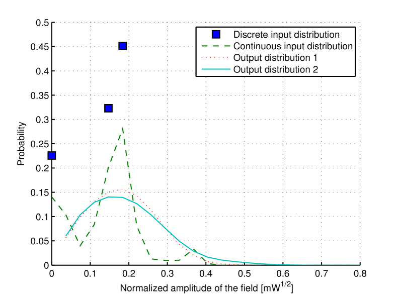
Figure 8: Capacity-achieving input and output distributions at SNR=2.6 dB. The noise power density is 1$\mu$W/GHZ and peak power ${\mathcal{P}}_{0}$=10 mW.

shows the capacity-achieving input distribution for the amplitude and the corresponding output distribution. Like the Rician fading channel, there is always a single mass point at the zero intensity with high probability. This is not unusual and exists in peak-constrained AWGN channels as well. Turning off the transmitter sufficiently frequently helps to stay within the given power budget, while mutual information is maximized over the remaining degrees of freedom. Like the AWGN channel, in low SNRs (SNR $<$6 dB), simple on-off keying (OOK) is near-optimal. In this case the channel is off more often than it is on. The ratio of on-to-off probabilities is 0.3 at SNR=2.5 dB, and decreases with increasing the SNR.

The surface of the mutual information as a function of the input probability distribution is flat around the optimum. Hence although the capacity optimization problem is a convex program with a unique optimum, there are distributions that come very close to the capacity but with quite different structure. With increasing SNR, the number of mass points and their locations increases. More powerful numerical methods are required to find discrete mass points at higher SNRs. We use the solution of the interior-point method as an starting point to search for discrete distributions using a second layer of interior-point optimization. The combined method was used to find discrete mass points at SNR=13 dB in Fig. 9.

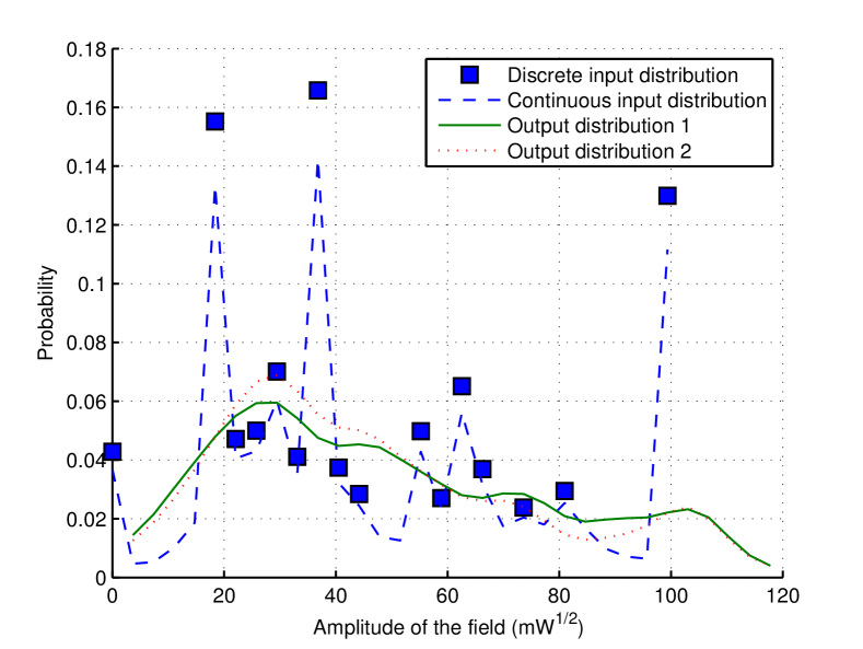
Figure 9: Capacity-achieving input and output distributions at SNR=13 dB. The noise power density is 1$\mu$W/GHZ and peak power ${\mathcal{P}}_{0}$=10 mW

Note that the number of mass points increases considerably beyond the low power region SNR$>$6 dB. Some of the points may be merged with a slight capacity loss. Indeed the controlled increase of the power shows that new mass points are created by splitting a single mass point with high probability into two new mass points. With no peak power, new mass points might come from infinity as conjectured in [22] for Rayleigh fading channel under average power constraint.

It is interesting to note that even though the capacity-achieving input distribution is not unique (in the sense that semi-continuous distributions are near-optimal within our affordable numerical accuracy), the output distribution appears to be unique. This can be observed in Fig. 8 and Fig. 9, where the corresponding output distribution is plotted for a discrete and semi-continuous input distribution. Capacity deviates $\pm$0.1 bits/symbol which is less than 4% error.

X Conclusion

We have considered the capacity of the per-sample channels that arise from a model of dispersion-free optical fibers. The capacity and capacity-achieving input distribution were evaluated numerically. We observed that the signal phase carries little or no information at very low and at very high signal-power levels, an observation that enabled us to find a simple lower bound on the capacity of the dispersion-free fiber which is asymptotically exact. Although the overall capacity subject to the average power constraint does not have a peak in its ${\mathcal{C}}$-${\mathcal{P}}$ curve and grows indefinitely with input signal power, there exists an optimal power for which the phase channel reaches its maximum bits/symbol capacity. For zero-dispersion fibers, neglecting spectral broadening may lead to wrong conclusions regarding the asymptote of the spectral efficiency.

Appendix A A stochastic calculus approach for the derivation of the conditional PDF

In this appendix we provide a different approach for the derivation of the conditional PDF of $Q(z)$ in the per-sample channel model (2), namely, $f_{Q(z)|Q(0)}(q(z)|q(0))$. The method is based on simple mathematical techniques for manipulating random differential equations, i.e., methods of the stochastic calculus (see e.g., [10]).

A-A Itô calculus

We start by separating the real and imaginary components of $Q(z)$ in (2), writing

$$\frac{\partial X_{1}(z)}{\partial z} = -\gamma X_{2}(X_{1}^{2}+X_{2}^{2})+V_{1}(z),$$

$$\frac{\partial X_{2}(z)}{\partial z} = \gamma X_{1}(X_{1}^{2}+X_{2}^{2})+V_{2}(z),$$ (44)

where $X_{1}(z)=\Re Q(z)$, $X_{2}(z)=\Im Q(z)$, and $V_{i}(z)$, $i=1,2$, are two independent zero-mean real Gaussian processes with $\mathsf{E}(V_{i}(z)V_{i}(z^{\prime}))=(\sigma^{2}/2)\delta(z-z^{\prime})$.

Note that, in strict mathematical terms, channel model (2) (or (A-A)) does not exist. To see this, let $\gamma$ be zero in (2). Solution of the equation is then $W(z)=\int_{0}^{z}V(z^{\prime})dz^{\prime}$, i.e., the Wiener process. The Wiener process is, however, known to be differentiable nowhere, to satisfy $\partial W/\partial z=V(z)$. To resolve this issue, stochastic differential equation (2) should be interpreted via its equivalent integral representation

$$Q(z)=Q_{0}+\int_{0}^{z}\gamma|Q|^{2}Qdz^{\prime}+\int_{0}^{z}V(z^{\prime})dz^{\prime}.$$ (45)

This eliminates problems with differentiating a stochastic process (one could also live in the Schwartz space of distributions and consider the original differential equation in the weak sense).

The system of stochastic differential equations (A-A) can be transformed to polar coordinates via the transformation

$$R=\sqrt{X_{1}^{2}+X_{2}^{2}},\quad\Phi=\tan^{-1}\frac{X2}{X1}.$$ (46)

However since (A-A) is a stochastic system, such a transformation cannot be executed simply based on the ordinary calculus.

Roughly speaking, the difference between the classical deterministic calculus and the stochastic calculus stems from the fact that, unlike the classical calculus in which terms proportional to ${\rm d}t^{2}$ are ignored, we can not neglect ${\rm d}W^{2}$ (square of infinitesimal increments of the Wiener process) in stochastic equations. Intuitively, this is because ${\rm d}W\sim\mathcal{N}_{\mathbb{C}}(0,\sigma^{2}dz)$ and therefore $\mathsf{E}({\rm d}W^{2})=\sigma^{2}dz$, i.e., ${\rm d}W^{2}$ is of order $dz$ and cannot be neglected. To see this more precisely, let us integrate the equation of $X_{1}(z)$ in (A-A) from $z$ to $z+\Delta z$ for small $\Delta z$

$$X_{1}(z+\Delta z)-X_{1}(z) \approx -\gamma X_{2}(z)\left(X_{1}(z)^{2}+X_{2}(z)^{2}\right)\Delta z$$

$$+\int_{z}^{z+\Delta z}V_{1}(z^{\prime})dz^{\prime}.$$

Following the classical calculus, the second term $\int_{z}^{z+\Delta z}V_{1}(z^{\prime})dz^{\prime}$ is approximated by $V_{1}(z)\Delta z$, similar to the first term. However, it is a fact that the variance of the summation of a sequence of independent random variables is the summation of the individual variances. In other words, the linearity is on the variance, not the standard deviation or the radius of the balls (signal level). Therefore, the second term properly is approximated by $V_{1}(z)\sqrt{\Delta z}$ which consequently affects the chain rule for differentiation. This can be also understood from the fact that, when one discretizes the differential equation (2) at points $z_{k}=k\epsilon$, the continuous-space stochastic process $V(z)$ is replaced by a sequence of random variables $\left\{\frac{V_{k}}{\sqrt{\epsilon}}\right\}$, where $V_{k}$ is a sequence of i.i.d zero-mean Gaussian random variables with $\mathsf{E}|V_{k}|^{2}=\sigma^{2}$.

In (45), any stochastic integral of the form $\int_{0}^{z}G(Q(z^{\prime}),z^{\prime})V(z^{\prime})dz^{\prime}$ is understood by definition as

$$\textnormal{mean-square}\lim\limits_{n\rightarrow\infty}\sum\limits_{k=1}^{n}G(Q(\tau_{k}),\tau_{k})\left(W(z^{\prime}_{k})-W(z^{\prime}_{k-1})\right),$$ (47)

where $\textnormal{mean-square}\lim$ is the mean square probabilistic limit, $z^{\prime}_{0}=0<z^{\prime}_{1}<\cdots<z^{\prime}_{n}=z$ is a partition of the interval $[0,z]$, and $z^{\prime}_{k-1}\leq\tau_{k}\leq z^{\prime}_{k}$. Unlike the classical calculus, the choice of the intermediate point $\tau_{k}\in[z^{\prime}_{k-1},z^{\prime}_{k}]$ affects the result of integration. Choosing $\tau_{k}=z^{\prime}_{k-1}$ leads to Itô’s interpretation of the stochastic integral, while using $\left\{G(Q(\tau_{k}),\tau_{k-1})+G(Q(\tau_{k-1}),\tau_{k-1})\right\}/2$ in (47) instead of $G(Q(\tau_{k}),\tau_{k})$, gives Stratonovich’s definition. As common in this context, in this paper we adopt Itô’s definition, which consequently leads to Itô calculus.

The following lemma is used when changing variables in a stochastic differential equation.

Lemma 2 (Itô’s lemma).

Let $\textbf{X}(z)$ be an n-dimensional stochastic process evolving according to the following first order stochastic differential equation

$${\rm d}\textbf{X}=\textbf{a}(\textbf{X},z){\rm d}z+{\sf{B}}(\textbf{X},z){\rm d}\textbf{W}(z),$$ (48)

where $\textbf{a}(\textbf{X},z)\in\mathbb{C}^{n}$ and ${\sf{B}}(\textbf{X},z)\in\mathbb{C}^{n\times n}$ are respectively vector-valued and matrix-valued functions, and elements of ${\rm d}\textbf{W}(z)$ are infinitesimal increments of independent Wiener processes with

$$\mathsf{E}\{W_{i}(z)W_{i}^{*}(z^{\prime})\}=\min(z,z^{\prime}),\quad i=1,\cdots,n.$$

Then for any twice continuously differentiable function $g(\textbf{X},z)$

$${\rm d}g(\textbf{X},z) = \biggl{\{}\dot{g}(\textbf{X},z)+\sum\limits_{i}\textbf{a}_{i}(\textbf{X},z)\partial_{i}g(\textbf{X},z)$$ (49)

$$+\>\frac{1}{2}\sum\limits_{i,j}[{\sf{B}}(\textbf{X},z){\sf{B}}(\textbf{X},z)^{T}]_{ij}\partial_{i}\partial_{j}g(\textbf{X},z)\biggr{\}}{\rm d}z$$

$$+\>\sum\limits_{i,j}{\sf{B}}_{ij}(\textbf{X},z)\partial_{i}g(\textbf{X},z){\rm d}W_{j}(z),$$

where $\dot{g}(\textbf{X},z)=\partial g(\textbf{X},z)/\partial z$, and $\partial_{i}$ stands for ordinary partial differentiation with respect to $\textbf{X}_{i}$.

Proof:

See [10]. ∎

In the context of statistical physics, the first order stochastic dynamical system (48) is called the nonlinear Langevin equation. The quantities $\textbf{a}(\textbf{X},z)$ and ${\sf{B}}(\textbf{X},z)$ are drift and diffusion coefficients. Note that the term $\frac{1}{2}\sum\limits_{i,j}[{\sf{B}}(\textbf{X},z){\sf{B}}(\textbf{X},z)^{T}]_{ij}\partial_{i}\partial_{j}g(\textbf{X},z)$ can be obtained only via the Itô calculus (unless $\textbf{a}(\textbf{X},z)$ is linear in X).

In the case of (A-A), ${\sf{B}}(\textbf{X},z)=\frac{\sigma}{\sqrt{2}}{\sf{I}}_{2}$, and all other constants are easily extracted from (A-A). Applying Lemma 2 to (46), the per-sample model (2) is properly transformed to polar coordinates

$$\begin{pmatrix}\frac{\partial R}{\partial z}\\ \frac{\partial\Phi}{\partial z}\end{pmatrix} = \begin{pmatrix}\overset{\textrm{Ito calculus}}{\overbrace{\frac{\sigma^{2}}{4R}}}\\ \gamma R^{2}\end{pmatrix}$$ (50)

$$+\>\frac{\sigma}{\sqrt{2}}\begin{pmatrix}\cos\Phi&\sin\Phi\\ -\sin\Phi/R&\cos\Phi/R\end{pmatrix}\begin{pmatrix}V_{1}\\ V_{2}\end{pmatrix}.$$

Note that in (50) we have assumed

$$\mathsf{E}\{V_{i}(z)V_{i}(z^{\prime})\}=\delta(z-z^{\prime}),\quad i=1,\cdots,n,$$ (51)

to be consistent with the statement of the Lemma 2, in which the amplitude of impulse functions is unit.

The radial diffusion term $\frac{\sigma^{2}}{4R}$ is the term which cannot be obtained by classical calculus and significantly changes the results. The new channel in the polar coordinates (50) is itself another Langevin equation whose parameters can be extracted from (50).

A-B Fokker-Planck equation

Consider now the Langevin equation (50), in which the stochastic process $\textbf{X}(z)=[R,\Phi]^{T}$ evolves in the distance dimension $z$. For a fixed $z$, $\textbf{X}(z)$ is a random variable with a probability density function $f_{\textbf{X}}(\textbf{x},z)$ parametrized by $z$. Since for the information-theoretic purposes we are not interested in correlation between intermediate space samples of random process, e.g., $\mathsf{E}\{\textbf{X}_{i}(z)\textbf{X}_{j}(z^{\prime})^{H}\}$, $0<z<z^{\prime}<{\mathcal{L}}$, a single conditional PDF at the output of the fiber completely describes the underlying channel. The stochastic process contains much more information, but this is irrelevant to our application.

Let $g(\textbf{X},z)$ be a general function in Lemma 2, independent of $z$, and with vanishing boundary terms in $\textbf{X}_{i}$ (i.e., if the support of densities extends to infinity, then $g(\pm\infty,z)=0$). One can look at the evolution of $\mathsf{E}g(\textbf{X},z)$, which is deterministic. The result is a deterministic equation in terms of $g(\textbf{X},z)$ and $f_{\textbf{X}}(\textbf{x},z)$. Since $g$ can be varied to be any change of variable, it follows that $f_{\textbf{X}}(\textbf{x},z)$ should satisfy a certain evolution equation. Let, therefore, fix $\textbf{X}=\textbf{x}$ in (49), multiply both sides of (49) by $f_{\textbf{X}}(\textbf{x},z)$, i.e., the PDF of $\textbf{X}(z)$ at a fixed $z$, and integrate with respect to x. Both sides can then be integrated by parts which transfers differentials from $g(\textbf{x},z)$ to $f_{\textbf{X}}(\textbf{x},z)$. Since the resulting integral holds for any $g(\textbf{x},z)$, the following lemma is obtained (for the case $n=1$).

Lemma 3 (Nonlinear Fokker-Planck equation).

Let $f_{\textbf{X}}(\textbf{x},z)$ be the probability density function of $\textbf{X}(z)$ at a fixed $z$ in the Langevin equation (48). Then $f_{\textbf{X}}(\textbf{x},z)$ satisfies the following differential equation

$$\frac{\partial f_{\textbf{X}}(\textbf{x},z)}{\partial z} = -\sum\limits_{i}\frac{\partial}{\textbf{x}_{i}}[\textbf{a}(\textbf{x},z)f_{\textbf{X}}(\textbf{x},z)]$$ (52)

$$+\>\frac{1}{2}\sum\limits_{i,j}\frac{\partial^{2}}{\partial\textbf{x}_{i}\partial\textbf{x}_{j}}\left\{[{\sf{B}}(\textbf{x},z){\sf{B}}(\textbf{x},z)^{T}]_{ij}f_{\textbf{X}}(\textbf{x},z)\right\}.$$

Proof:

For the single variable case, the proof outlined above simply gives the desired result. The generalization to the multivariable case is, however, complicated since boundary terms are now surfaces and curves, instead of points. See [10] for the complete proof. ∎

Description of the probability density function via the Fokker Planck equation is incomplete without specifying the boundary conditions. In the multivariable case, such conditions may render the problem hard to solve analytically. In this paper, we assume

$$f_{\textbf{X}}(\textbf{x},z=0)=\delta(q-q_{0}),\quad\lim\limits_{|\textbf{x}|_{i}\rightarrow\infty}f_{\textbf{X}}(\textbf{x},z)=0,\quad\forall i.$$

The delta function implies that we are looking for the conditional PDF $f_{\textbf{X}}(\textbf{x},z|\textbf{x}_{0},z_{0})$. In the following, we unambiguously use $f_{\textbf{X}}(\textbf{x},z)$ instead of $f_{\textbf{X}}(\textbf{x},z|\textbf{x}_{0},z_{0})$ for the sake of brevity. Depending on the structure of the problem, other appropriate boundary conditions might be assumed, such as periodic, absorbing or reflecting boundary conditions.

Note that according to the Fokker-Planck equation, matrix ${\sf{B}}(\textbf{X},z)$ in the dynamics of the stochastic process affects the PDF in the form of ${\sf{B}}(\textbf{X},z){\sf{B}}(\textbf{X},z)^{T}$. In other words, probabilistically channel (50) is equivalent to

$$\begin{pmatrix}\frac{\partial R}{\partial z}\\ \frac{\partial\Phi}{\partial z}\end{pmatrix} = \begin{pmatrix}\frac{\sigma^{2}}{4R}\\ \gamma R^{2}\\ \end{pmatrix}+\>\frac{\sigma}{\sqrt{2}}\begin{pmatrix}1&0\\ 0&\frac{1}{R^{2}}\end{pmatrix}\begin{pmatrix}V_{1}\\ V_{2}\end{pmatrix},$$ (53)

which corresponds to the following Fokker-Planck equation

$$\frac{\partial f(r,\phi,z)}{\partial z} = -\gamma r^{2}\frac{\partial f}{\partial\phi}+\frac{1}{4}\sigma^{2}\left[\frac{\partial^{2}f}{\partial r^{2}}+\frac{1}{r^{2}}\frac{\partial^{2}f}{\partial\phi^{2}}\right]$$ (54)

$$-\>\overset{\textrm{Ito term}}{\overbrace{\frac{\sigma^{2}}{4}\frac{\partial}{\partial r}\left(\frac{f}{r}\right)}},$$

$$f(r,\phi,0) = \delta(r-r_{0},\phi-\phi_{0}).$$

Remark 3 (Phase Symmetry).

If $f(r,\phi,z)$ is a solution of (54), so is $f(r,\phi-\phi_{1},z)$ for any $\phi_{1}$. The PDF is therefore symmetric with respect to the phase, i.e., it is a function of $\phi-\phi_{0}$. This essentially comes from the fact that in the nonlinear Schrödinger equation, the cubic nonlinearity is of the form $|Q|^{2}Q$, as opposed to $Q^{3}$. This roots back to the underlying physics of the fiber, in which the nonlinear refractive response of the silica glass to an external light beam is deterministically proportional to the intensity $|Q|^{2}$ of the incoming beam. The absolute value is responsible for some very important properties of the nonlinear Schrödinger equation.

We proceed to solve the resulting partial differential equation (54). First, we find the marginal PDF of the amplitude channel alone. Integrating both sides of (54) with respect to $\phi$ in the interval $[0,2\pi]$, assuming phase continuity $f(r,0,z)=f(r,2\pi,z)$, and performing phase marginalization, we obtain

$$\frac{\partial f(r,z)}{\partial z} = \frac{1}{4}\sigma^{2}\frac{\partial^{2}f(r,z)}{\partial r^{2}}-\frac{\sigma^{2}}{4}\frac{\partial}{\partial r}\left[\frac{f(r,z)}{r}\right],$$ (55)

$$f(r,0) = \delta(r-r_{0}).$$

The PDF of the amplitude, $f(r,z)$, satisfies (55). If at $z=0$, $r=r_{0}$, then the conditional PDF $f(r,z|r_{0})$ is the solution of (55). We make the following observations about the resulting PDE.

Remark 4 (Scaling Property).

Partial differential equation (55) admits an important scaling property: if $f(r,z|r_{0})$ is a solution of (55), then so is $f(\lambda r,\lambda^{2}z|\lambda r_{0})$ for any real nonzero $\lambda$. Such scaling is indeed a Lie symmetry group of the partial differential equation (55) and corresponds to a conserved quantity. The essential feature of the symmetry group is that it conserves the set of solutions of the differential equation, inducing a set of orbits under action by the group. Each symmetry group may be visualized as permuting integral curves of the partial differential equation among themselves.

Remark 5 (Robustness).

The PDF of the amplitude does not depend on the Kerr nonlinearity constant $\gamma$, hence the operation of an amplitude detector (e.g., a photodetector) is also independent of $\gamma$.

We use the scaling property in Remark 4 to solve the partial differential equation (55). Such scaling implies that the ratios $r^{2}/z$ and $rr_{0}/z$ are important quantities for the equation (55). We therefore search for the solutions of the form $f(r,z)=h(\frac{r^{2}}{z},\frac{rr_{0}}{z})$. Substituting this into (55) and after straightforward algebra, we obtain the solution

$$f(r,z)=\frac{2r}{\sigma^{2}z}e^{-\frac{r^{2}+r_{0}^{2}}{\sigma^{2}z}}I_{0}\left(\frac{rr_{0}}{\sigma^{2}z}\right),$$ (56)

where we have scaled $f$ so that it stands for a probability distribution, and $f\rightarrow\delta(r-r_{0})$ when $z\rightarrow 0$ ( if $z\rightarrow 0$, then $I_{0}(\frac{2rr_{0}}{\sigma^{2}z})\rightarrow\frac{1}{r}\sqrt{\frac{\sigma^{2}z}{2\pi}}e^{\frac{2rr_{0}}{\sigma^{2}z}}$). Below we use (56) to solve (54). Note that alternatively one may solve (55) using Remark 5: since the PDF of the amplitude does not depend on $\gamma$, one can assume $\gamma=0$ in the original equation $\eqref{eq:zerodis}$ and find the PDF of the amplitude of a complex Brownian motion.

We use the method of separation of variables to solve the PDE (54). Assuming $f$ is separable in $r$ and $\phi$, i.e.,

$$f(r,\phi,z)=g(r,z)h(\phi,z),$$ (57)

and plugging (57) into (54), we get

$$\frac{1}{g}\frac{\partial g(r,z)}{\partial z}+\frac{1}{h}\frac{\partial h(\phi,z)}{\partial z}=-\gamma r^{2}\frac{1}{h(\phi,z)}\frac{\partial h(\phi,z)}{\partial\phi}$$

$$+\>\frac{1}{4}D\biggl{\{}\frac{1}{g(r,z)}\frac{\partial^{2}g(r,z)}{\partial r^{2}}+\frac{1}{r^{2}}\frac{1}{h(r,z)}\frac{\partial^{2}h(\phi,z)}{\partial\phi^{2}}$$

$$-\frac{1}{g(r,z)}\frac{\partial}{\partial r}(\frac{g(r,z)}{r})\biggr{\}}.$$ (58)

If

$$\frac{1}{h(\phi,z)}\frac{\partial h(\phi,z)}{\partial\phi}=c$$ (59)

for some constant $c$, then

$$\frac{1}{h(\phi,z)}\frac{\partial^{2}h(\phi,z)}{\partial\phi^{2}}=c^{2}.$$

In this case, (A-B) allows a separation of variables. Solution of the phase part in (59) is $h(\phi,z)=\exp\left[c\left(\phi-\phi_{0}\right)\right]$ and the equation for the amplitude part, $g(r,z)$, is

$$\frac{\partial g_{c}}{\partial z}=\frac{\sigma^{2}}{4}\frac{\partial^{2}g_{c}}{\partial r^{2}}+\left(\frac{c^{2}}{r^{2}}\frac{\sigma^{2}}{4}-\gamma cr^{2}\right)g_{c}-\frac{\sigma^{2}}{4}\frac{\partial}{\partial r}\left(\frac{g_{c}}{r}\right).$$ (60)

Due to phase periodicity, naturally one can assume $c=jm$, whence the PDF is written as a Fourier series with coefficient $g_{m}(z,r)$.

Although (60) is linear in $g_{c}$, applying Fourier or Laplace transform gives another PDE which is as hard as (60) to solve. We prefer to use a variational method. If $c=0$, (60) is reduced to (55) whose solution is then (56). We therefore assume the general solution for $c\neq 0$ to be a variation of the solution at $c=0$,

$$g_{c}(r,z)=\frac{r}{\pi\sigma^{2}z}e^{-\left(r^{2}+r_{0}^{2}\right)a(z)}I_{m}(2rr_{0}b(z))$$ (61)

for some unknown $a(z)$ and $b(z)$ to be determined. Finally, $\eqref{eq:gc-candid}$ is plugged in (60) to get differential equations for $a(z)$ and $b(z)$. After some rather tedious but straightforward algebra, the overall PDF

$$f(r,z)=\sum\limits_{m=-\infty}^{\infty}e^{jm(\phi-\phi_{0}-\gamma r_{0}^{2}z)}g_{m}(r,z)$$

is obtained, in which

$$g_{m}(r,z)=\frac{rb(m)}{\pi}e^{-a_{m}(z)\left(r^{2}+r_{0}^{2}\right)}I_{|m|}(2b_{m}(z)r_{0}r),$$

where

$$a_{m}(z) = \frac{\sqrt{jm\gamma}}{\sigma}\coth\sqrt{jm\gamma\sigma^{2}}z,$$

$$b_{m}(z) = \frac{\sqrt{jm\gamma}}{\sigma}\frac{1}{\sinh\sqrt{jm\gamma\sigma^{2}}z}.$$

Functions $g_{m}(r,z)$ can be considered as eigenfunctions in the amplitude PDE (60), $\partial g/\partial z=Hg=\lambda g$ (see the literature in time-dependent Schrödinger equation in quantum mechanics). The PDF (18) then appears to be an expansion in terms of eigenfunctions of the associated Fokker-Planck equation. Each of these terms is a solution of the Fokker-Planck equation and the summation in (18) is to create the delta function $\delta(\phi-\phi_{0})$ at the beginning of the fiber.

As this paper was going to press, we became aware that a similar Fokker-Planck approach to describing the statistics of the model (2) has been worked out—in the context of nonlinear oscillators—in [25].

Appendix B Useful identities

$$\frac{1}{2\pi}\int\limits_{0}^{2\pi}e^{-jm\theta+x\cos(\theta-\theta_{0})}d\theta = I_{m}(x)e^{-jm\theta_{0}}$$ (62)

$$\int\limits_{0}^{\infty}xe^{-ax^{2}}I_{m}(bx)I_{m}(cx)dx = \frac{1}{2a}e^{\frac{b^{2}+c^{2}}{4a}}I_{m}(\frac{bc}{2a})$$ (63)

Frank R. Kschischang received the B.A.Sc. degree (with honors) from the University of British Columbia, Vancouver, BC, Canada, in 1985 and the M.A.Sc. and Ph.D. degrees from the University of Toronto, Toronto, ON, Canada, in 1988 and 1991, respectively, all in electrical engineering. He is a Professor of Electrical and Computer Engineering at the University of Toronto, where he has been a faculty member since 1991. During 1997-98, he was a visiting scientist at MIT, Cambridge, MA and in 2005 he was a visiting professor at the ETH, Zurich. His research interests are focused primarily on the area of channel coding techniques, applied to wireline, wireless and optical communication systems and networks. In 1999 he was a recipient of the Ontario Premier’s Excellence Research Award and in 2001 (renewed in 2008) he was awarded the Tier I Canada Research Chair in Communication Algorithms at the University of Toronto. In 2010 he was awarded the Killam Research Fellowship by the Canada Council for the Arts. Jointly with Ralf Koetter he received the 2010 Communications Society and Information Theory Society Joint Paper Award. He is a Fellow of IEEE and of the Engineering Institute of Canada. During 1997-2000, he served as an Associate Editor for Coding Theory for the IEEE TRANSACTIONS ON INFORMATION THEORY. He also served as technical program co-chair for the 2004 IEEE International Symposium on Information Theory (ISIT), Chicago, and as general co-chair for ISIT 2008, Toronto. He served as the 2010 President of the IEEE Information Theory Society.

References

- [1] P. P. Mitra and J. B. Stark, “Nonlinear limits to the information capacity of optical fiber communications,” Letters to Nature, vol. 411, pp. 1027–1030, 2000.
- [2] J. Tang, “The Shannon channel capacity of dispersion-free nonlinear optical fiber transmission,” J. Lightw. Technol., vol. 19, no. 8, pp. 1104–1109, 2001.
- [3] E. E. Narimanov and P. Mitra, “The channel capacity of a fiber optics communication system: perturbation theory,” J. Lightw. Technol., vol. 20, no. 3, pp. 530–537, 2002.
- [4] R. J. Essiambre, G. Kramer, P. J. Winzer, G. J. Foschini, and B. Goebel, “Capacity limits of optical fiber networks,” J. Lightw. Technol., vol. 28, no. 4, pp. 662–701, February 2010.
- [5] K. S. Turitsyn, S. A. Derevyanko, I. V. Yurkevich, and S. K. Turitsyn, “Information capacity of optical fiber channels with zero average dispersion,” Phys. Rev. Lett., vol. 91, no. 20, p. 203901, 2003.
- [6] J. M. Kahn and K.-P. Ho, “Spectral efficiency limits and modulation/detection techniques for DWDM systems,” IEEE. J. Sel. Topics Quantum Electron., vol. 10, no. 2, pp. 259–272, Mar./Apr. 2004.
- [7] A. Mecozzi, “Limits to long-haul coherent transmission set by the Kerr nonlinearity and noise of the in-line amplifiers,” J. Lightw. Technol., vol. 12, no. 11, pp. 1993–2000, 1994.
- [8] A. Mecozzi and M. Shtaif, “On the capacity of intensity modulated systems using optical amplifiers,” IEEE Photon. Technol. Lett., vol. 13, no. 9, pp. 1029–1031, 2001.
- [9] S. M. Moser, “Duality-based bounds on channel capacity,” Ph.D. dissertation, ETH Zurich, Switzerland, 2004.
- [10] C. W. Gardiner, Handbook of Stochastic Methods for Physics, Chemistry, and the Natural Sciences. Springer-Verlag New York, 1985.
- [11] M. N. Islam, Raman Amplifiers for Telecommunications: Sub-systems and systems. Springer, 2003.
- [12] R. P. Feynman and A. R. Hibbs, Quantum Mechanics and Path Integrals, McGraw-Hill, 1965.
- [13] J. Zinn-Justin, Quantum Field Theory and Critical Phenomena. Oxford University Press, 2002.
- [14] G. P. Agrawal, Nonlinear Fiber Optics. Springer, 2006.
- [15] R. E. Blahut, “Computation of channel capacity and rate-distortion functions,” IEEE Trans. Inf. Theory, vol. 18, no. 4, pp. 460–473, July 1972.
- [16] S. Boyd and L. Vandenberghe, Convex Optimization. Cambridge University Press, 2004.
- [17] K. P. Ho, “Probability density of nonlinear phase noise,” J. Opt. Soc. Amer. B., vol. 20, no. 9, pp. 1875–1879, 2003.
- [18] I. S. Gradštejn, I. M. Ryžik, A. Jeffrey, and D. Zwillinger, Table of Integrals, Series, and Products, 6th ed. Academic Press, 2000.
- [19] Characteristics of a single-mode optical fibre and cable. ITU-T Recommendation G.652, International Telecommunication Union (ITU), 2000.
- [20] Characteristics of a dispersion-shifted single-mode optical fibre and cable. ITU-T Recommendation G.653, International Telecommunication Union (ITU), 1997.
- [21] S. Shamai and I. Bar-David, “The capacity of average and peak-power-limited quadrature Gaussian channels,” IEEE Trans. Inf. Theory, vol. 41, no. 4, pp. 1060–1071, 1995.
- [22] I. C. Abou-Faycal, M. D. Trott, and S. Shamai, “The capacity of discrete-time memoryless Rayleigh-fading channels,” IEEE Trans. Inf. Theory, vol. 47, no. 4, pp. 1290–1301, 2001.
- [23] T. H. Chan, S. Hranilovic, and F. R. Kschischang, “Capacity-achieving probability measure for conditionally Gaussian channels with bounded inputs,” IEEE Trans. Inf. Theory, vol. 51, no. 6, pp. 2073–2088, 2005.
- [24] M. C. Gursoy, H. V. Poor, and S. Verdu, “The noncoherent Rician fading channel-part I: structure of the capacity-achieving input,” IEEE Trans. on Wireless Commun., vol. 4, no. 5, pp. 2193–2206, 2005.
- [25] J. E. Prilepsky and S. A. Derevyanko, “Statistics of noise-driven coupled nonlinear oscillators: Applications to systems with Kerr nonlinearity,” Physica D, vol. 203, pp. 249–269, 2005.