The Numerical Simulation of Ship Waves
using Cartesian Grid Methods

Abstract

Two different cartesian-grid methods are used to simulate the flow around the DDG 5415. The first technique uses a “coupled level-set and volume-of-fluid” (CLS) technique to model the free-surface interface. The no-flux boundary condition on the hull is imposed using a finite-volume technique. The second technique uses a level-set technique (LS) to model the free-surface interface. A body-force technique is used to impose the hull boundary condition. The predictions of both numerical techniques are compared to whisker-probe measurements of the DDG 5415. The level-set technique is also used to investigate the breakup of a two-dimensional spray sheet.

1 Introduction

At moderate to high speed, the turbulent flow along the hull of a ship and behind the stern is characterized by complex physical processes which involve breaking waves, air entrainment, free-surface turbulence, and the formation of spray. Traditional numerical approaches to these problems, which use boundary-fitted grids, are difficult and time-consuming to implement. Also, as waves steepen, boundary-fitted grids will break down unless ad hoc treatments are implemented to prevent the waves from getting too steep. At the very least, a bridge is required between potential-flow methods, which model limited physics, and more complex boundary-fitted grid methods, which incorporate more physics, albeit with great effort and with limitations on the wave steepness. Cartesian-grid methods are a natural choice because they allow more complex physics than potential-flow methods, and, unlike boundary-fitted methods, cartesian-grid methods require minimal effort with no limitation on the wave steepness. Although cartesian-grid methods (CGM) are presently incapable of resolving the hull boundary-layer, CGM can model wave breaking, free-surface turbulence, air entrainment, spray-sheet formation, and complex interactions between the ship hull and the free surface, such as transom-stern flows and tumblehome bows. The cartesian-grid methods that are described in this paper use the panelized geometry that is used by potential-flow methods to automatically construct a representation of the hull. The hull representation is then immersed inside a cartesian grid that used to track the interface. No additional gridding beyond what is already used by potential-flow methods is required. We note that another variation of this approach is to use cartesian-grid methods to track the free-surface interface and body-fitted grids to model the ship hull.

For the calculation of ship waves, VOF and level-set methods have certain advantages and disadvantages. VOF uses the volume fraction ($F$) to track the interface. $F=0$ corresponds to gas and $F=1$ corresponds to liquid. For intermediate values, between zero and one, there exists an interface between the gas and the liquid. The interface between the gas and the liquid is sharp for a pure VOF method. Level-set methods use a level-set function ($\phi$) to model the gas-liquid interface. By definition, $\phi<0$ denotes gas, $\phi>0$ denotes liquid, and $\phi=0$ is the interface. For conventional level-set schemes, the interface between the gas and the liquid is given a finite thickness[17], which is unlike conventional VOF schemes[3].

In the case of free-surface flows, where the density ratio between air and water is almost three orders of magnitude, the finite thickness of the interface that characterizes level-set methods has two advantages over VOF. First, the finite thickness tends to smooth jumps in the tangential component of the velocity on the interface. Second, the finite thickness tends to facilitate using multigrid methods to solve various types of elliptic equations that involve the density.

The advection algorithm that is used for VOF conserves mass if the flow field is solenoidal. The level-set advection equation tends to accumulate numerical errors. For the level-set method, the level-set function must be periodically reinitialized to maintain a proper thickness for the interface, otherwise the interface would become either too thick or too thin. The reinitialization process is a significant source of errors in the level-set method. Based on accuracy considerations, the calculation of gravity-driven flows tends to favor VOF over level-set methods.

The interface is reconstructed from the volume fractions in VOF. During the reconstruction process, the interface normals and curvature are calculated. Typically, the calculation of the interface normal and curvature are less accurate for VOF than for level-set methods. The interface normals and curvature are calculated directly in level-set methods in terms of gradients of the level-set function. As a result, the calculation of the normals and curvature are less costly for level-set methods relative to VOF. The calculation of surface tension effects, which are a function of the curvature of the interface, tends to favor level-set methods over VOF due to considerations of accuracy and efficiency.

On highly-stretched, multidimensional grids, VOF methods are less prone to aliasing errors than level-set methods. Level-set methods incur errors as the interface rotates through highly resolved regions into regions that are not resolved well. This type of aliasing error occurs in cartesian-grid methods when the mesh along one coordinate axis is more finely resolved than along another coordinate axis.

By definition, the level-set and volume-of-fluid function both allow mixing of gas and liquid. This feature of level-set and volume-of-fluid methods may be desirable for modeling gas entrainment such as the air that is entrained by a breaking wave. During the reinitialization process, level-set methods and “coupled level set and volume-of-fluid methods” (CLS) use a signed distance function to update the level-set function and the thickness of the interface. Naturally, the distance function could be used to model the intensity of turbulence and amount of gas entrainment as a function of the distance to the interface.

Dommermuth, et al., (1998) used a stratified flow formulation to simulate breaking bow waves on the DDG 5415 at a Froude number Fr=0.41. Their numerical results compared well to whisker-probe measurements in the bow region [8]. However, Dommermuth, et al., (1998) identified two issues that required further study. First, their stratified flow formulation allowed the free-surface interface to become too diffuse. Second, the contact-line treatment didnot allow the free surface to rise and fall cleanly along the side of the hull. The two new numerical approaches that are discussed in this paper are attempts to remedy these problems.

Both numerical approaches use a signed distance function to represent the hull. The distance of a point to the hull is negative inside the hull and positive outside the hull. The finite-volume approach uses the signed distance to calculate the area and volume fractions for computational cells cut by the hull, whereas the body-force technique uses the signed distance to prescribe a smooth forcing term. The coupled interface-tracking algorithm (CLS) uses level-set to calculate the normals (and curvature if needed) to the free-surface interface that are used in VOF. The advection portion of the algorithm is performed by VOF [16]. The level-set interface-tracking algorithm uses a new isosurface scheme to calculate the zero level-set. Then the minimal distance between the cartesian points and the zero level-set is calculated in a narrow band. The minimal distance is made positive in the water and negative in the air. This signed distance to the free surface is used to reinitialize the thickness of the interface.

The two numerical approaches are used to simulate the flow around the DDG 5415. The CLS technique is still under development, so only preliminary results are presented. The level-set technique includes upgrades to the numerical technique that is described in [8]. Those upgrades include a new body-force formulation that is mollified, a new reinitialization procedure, and a new finite-volume treatment of the convective terms. The original numerical procedure is not mollified and does not use reinitialization. In addition, the original central-difference formulation of the convective terms is not as robust as the new treatment using a flux integral formulation. We first review the governing equations and then we discuss the numerical approaches. Finally, we present some preliminary numerical results which illustrate various features of the numerical algorithms. The application of level-set methods to the breakup of spray sheets is also illustrated.

2 Field Equations

As in Dommermuth, et al., (1998), consider turbulent flow at the interface between air and water [8]. Let $u_{i}$ denote the three-dimensional velocity field as a function of space ($x_{i}$) and time ($t$). For an incompressible flow, the conservation of mass gives

$$\frac{\partial u_{i}}{\partial x_{i}}=0\;\;.$$ (1)

$u_{i}$ and $x_{i}$ are normalized by $U_{o}$ and $L_{o}$, which are the characteristic velocity and length scales of the body, respectively. On the surface of the moving body ($S_{b}$), the fluid particles move with the body:

$$u_{i}=U_{i}\;\;,$$ (2)

where $U_{i}$ is the velocity of the body.

Let $V_{\ell}$ and $V_{g}$ respectively denote the liquid (water) and gas (air) volumes. Following a procedure that is similar to [13, 15], we let $\phi$ denote a level-set function. By definition, $\phi=-1$ for ${\bf x}\in V_{g}$ and $\phi=1$ for ${\bf x}\in V_{\ell}$. The fluid interface corresponds to $\phi=0$.

The convection of $\phi$ is expressed as follows:

$$\frac{d\phi}{dt}=\frac{\partial Q}{\partial x_{j}}\;\;,$$ (3)

where $d/dt=\partial/\partial t+u_{i}\partial/\partial x_{i}$ is a substantial derivative. $Q$ is a sub-grid-scale flux which can model the entrainment of gas into the liquid. Details are provided in [8].

Let $\rho_{\ell}$ and $\mu_{\ell}$ respectively denote the density and dynamic viscosity of water. Similarly, $\rho_{g}$ and $\mu_{g}$ are the corresponding properties of air. The flow in the water and air is governed by the Navier-Stokes equations:

$$\frac{du_{i}}{dt} = F_{i}-\frac{1}{\rho}\frac{\partial P}{\partial x_{i}}+\frac{1}{\rho R_{e}}\frac{\partial}{\partial x_{j}}\left(2\mu S_{ij}\right)$$ (4)

$$-\frac{1}{F_{r}^{2}}\delta_{i3}+\frac{1}{\rho W_{e}}T_{i}+\frac{\partial\tau_{ij}}{\partial x_{j}}\;\;,$$

where $R_{e}=\rho_{\ell}U_{o}L_{o}/\mu_{\ell}$ is the Reynolds number, $F_{r}^{2}=U_{o}^{2}/(gL_{o})$ is the Froude number, and $W_{e}=\rho_{\ell}U_{o}^{2}L_{o}/\sigma$ is the Weber number. $g$ is the acceleration of gravity, and $\sigma$ is the surface tension. $F_{i}$ is a body force that is used to impose boundary conditions on the surface of the body. $P$ is the pressure. $T_{i}$ accounts for surface-tension effects. $\delta_{ij}$ is the Kronecker delta symbol. As described in [8], $\tau_{ij}$ is the subgrid-scale stress tensor. $S_{ij}$ is the deformation tensor:

$$S_{ij} = \frac{1}{2}\left(\frac{\partial u_{i}}{\partial x_{j}}+\frac{\partial u_{j}}{\partial x_{i}}\right)\;\;.$$ (5)

$\rho$ and $\mu$ are respectively the dimensionless variable densities and viscosities:

$$\rho(\phi) = \lambda+(1-\lambda){\rm H}(\phi)$$

$$\mu(\phi) = \eta+(1-\eta){\rm H}(\phi)\;\;,$$ (6)

where $\lambda=\rho_{g}/\rho_{\ell}$ and $\eta=\mu_{g}/\mu_{\ell}$ are the density and viscosity ratios between air and water. For a sharp interface, with no mixing of air and water, $H$ is a step function. In practice, a mollified step function is used to provide a smooth transition between air and water.

Based on [3, 4], the effects of surface tension are expressed as a singular source term in the Navier-Stokes equations:

$$T_{i}=\kappa(\phi)\frac{\partial}{\partial x_{i}}H(\phi)$$ (7)

where $\kappa$ is the curvature of the air-water interface expressed in terms of the level-set function:

$$\kappa(\phi)=\nabla\cdot\left(\frac{\nabla\phi}{|\nabla\phi|}\right)\;\;.$$ (8)

The pressure is reformulated to absorb the hydrostatic term:

$$P = P_{d}+P_{h}\;\;,$$ (9)

where $P_{d}$ is the dynamic pressure and $P_{h}$ is a hydrostatic pressure term:

$$P_{h} = -\int^{z}dz^{\prime}\rho(z^{\prime})\frac{1}{F_{r}^{2}}\;\;$$ (10)

As discussed in [8], the divergence of the momentum equations (4) in combination with the conservation of mass (1) provides a Poisson equation for the dynamic pressure:

$$\frac{\partial}{\partial x_{i}}\frac{1}{\rho}\frac{\partial P_{d}}{\partial x_{i}}=\Sigma\;\;,$$ (11)

where $\Sigma$ is a source term. Equation 11 is used to project the velocity onto a solenoidal field.

3 Enforcement of Body Boundary Conditions

Two different cartesian-grid methods are used to simulate the flow around the DDG 5415. The first technique imposes the no-flux boundary condition on the body using a finite-volume technique. The second technique imposes the no-flux boundary condition via an external force field. Both techniques use a signed distance function $\psi$ to represent the body. $\psi$ is positive outside the body and negative inside the body. The magnitude of $\psi$ is the minimal distance between the position of $\psi$ and the surface of the body.

With respect to the volume of fluid that is enclosed by the body ($V_{b}$), we define a function ${\cal F}$:

$${\cal F}({\bf x})=\left\{\begin{array}[]{l}1\;\;{\rm for}\;\;{\bf x}\in V_{b}\\ \frac{1}{2}\;\;{\rm for}\;\;{\bf x}\in S_{b}\\ 0\;\;{\rm for}\;\;{\bf x}\not\in V_{b}\end{array}\right.\;\;.$$ (15)

The function ${\cal F}$ can be expressed in terms of a surface distribution of normal dipoles [10].

$${\cal F}({\bf x}) = \frac{1}{4\pi}\int_{S_{b}}ds^{\prime}\frac{\partial}{\partial n^{\prime}}\frac{1}{R}\;\;,$$ (16)

where $n$ is the outward-pointing unit normal to the body, and $R$ is a Rankine source, $R=|{\bf x}-{\bf x}^{\prime}|$. $\psi$ is expressed in terms of ${\cal F}$ as follows,

$$\psi({\bf x})={\cal F}({\bf x})|{\bf x}-{\bf x}^{\prime}|_{min}\;\;,$$ (17)

where $|{\bf x}-{\bf x}^{\prime}|_{min}$ is the minimal distance between the field point ${\bf x}$ and the points on the body ${\bf x}^{\prime}$. In practice, the body is discretized using triangular panels. As a result, the calculation of the minimal distance sweeps over all the triangles comprising the body and must account for the possibility that the minimal distance may occur either at the corners of triangle, along the edges of triangle, or inside the triangle.

3.1 Free-slip conditions

In the finite volume approach, the irregular boundary (i.e. ship hull) is represented in terms of $\psi$ along with the corresponding area fractions $A$ and volume fractions $V$. $V=1$ for computational elements fully outside the body and $V=0$ for computational elements fully inside the body. The representation of irregular boundaries via area fractions and volume fractions has been used previously in the following work for incompressible flows [1, 19, 5].

Recall the pressure equation,

$$\nabla\cdot\frac{\nabla p}{\rho}=\nabla\cdot\mbox{\boldmath$W$\unboldmath}.$$ (18)

with the following no-flow boundary condition:

$$\frac{\nabla p}{\rho}\cdot\mbox{\boldmath$n$\unboldmath}_{wall}=\mbox{\boldmath$W$\unboldmath}\cdot\mbox{\boldmath$n$\unboldmath}_{wall}.$$ (19)

where $\mbox{\boldmath$n$\unboldmath}_{wall}$ is the outward normal drawn from the active flow region into the geometry region.

For each discrete computational element $\Omega_{i,j,k}$ we define the geometry volume fraction $V$ and area fraction $A$ as

$$V_{ijk}\equiv\frac{1}{|\Omega_{ijk}|}\int_{\Omega_{ijk}}H(\psi)d\mbox{\boldmath$x$\unboldmath}.$$

$$A_{i+1/2,j,k}\equiv\frac{1}{|\Gamma_{i+1/2,j,k}|}\int_{\Gamma_{i+1/2,j,k}}H(\psi)d\mbox{\boldmath$x$\unboldmath}.$$

$\Gamma_{i+1/2,j,k}$ represents the left face of a computational element; similar definitions apply to $\Gamma_{i-1/2,j,k}$, $\Gamma_{i,j+1/2,k}$, ….

In order to discretely enforce the boundary conditions (19) at the geometry surface, we use a finite volume approach for discretizing (18).

Given an irregular computational element $\Omega_{ijk}$ (see Figure 1), we have

$$\int_{\Omega_{ijk}}\nabla\cdot\mbox{\boldmath$U$\unboldmath}dV=\int_{\partial\Omega_{ijk}}\mbox{\boldmath$U$\unboldmath}\cdot\mbox{\boldmath$n$\unboldmath}_{wall}dA.$$

The divergence theorem motivates the following second order approximation of the divergence $\nabla\cdot\mbox{\boldmath$U$\unboldmath}$ at the centroid of $\Omega_{ijk}$:

$$\nabla\cdot\mbox{\boldmath$U$\unboldmath}\approx\frac{1}{|\Omega_{ijk}|}\int_{\partial\Omega_{ijk}}\mbox{\boldmath$U$\unboldmath}\cdot\mbox{\boldmath$n$\unboldmath}_{wall}dA.$$ (20)

In terms of geometry volume fractions $V_{ijk}$ and area fractions $A_{i+1/2,j,k}$, (20) becomes,

$$\nabla\cdot\mbox{\boldmath$U$\unboldmath}\approx\frac{1}{V_{ijk}\Delta x\Delta y\Delta z}[$$ (21)

$$(A_{i+1/2,j,k}\Delta y\Delta z)u_{i+1/2,j,k}-$$

$$(A_{i-1/2,j,k}\Delta y\Delta z)u_{i-1/2,j,k}+$$

$$(A_{i,j+1/2,k}\Delta x\Delta z)v_{i,j+1/2,k}-$$

$$(A_{i,j-1/2,k}\Delta x\Delta z)v_{i,j-1/2,k}+$$

$$(A_{i,j,k+1/2}\Delta x\Delta y)w_{i,j,k+1/2}-$$

$$(A_{i,j,k-1/2}\Delta x\Delta y)w_{i,j,k-1/2}-$$

$$L^{wall}_{ijk}\mbox{\boldmath$U$\unboldmath}^{wall}_{ijk}\cdot\mbox{\boldmath$n$\unboldmath}_{wall}].$$

For a zero flux boundary condition at the wall, the last term in (21), $L^{wall}_{ij}\mbox{\boldmath$U$\unboldmath}^{wall}_{ij}\cdot\mbox{\boldmath$n$\unboldmath}_{wall}$, is zero.

The finite volume approach, when applied to the divergence operator in (18) becomes:

$$\nabla\cdot\frac{1}{\rho}\nabla p\approx\frac{1}{V_{ijk}\Delta x\Delta y\Delta z}[$$

$$A_{i+1/2,j,k}\Delta y\Delta z(p_{x}/\rho)_{i+1/2,j,k}-$$

$$A_{i-1/2,j,k}\Delta y\Delta z(p_{x}/\rho)_{i-1/2,j,k}+$$

$$A_{i,j+1/2,k}\Delta x\Delta z(p_{y}/\rho)_{i,j+1/2,k}-$$

$$A_{i,j-1/2,k}\Delta x\Delta z(p_{y}/\rho)_{i,j-1/2,k}+$$

$$A_{i,j,k+1/2}\Delta x\Delta y(p_{z}/\rho)_{i,j,k+1/2}-$$

$$A_{i,j,k-1/2}\Delta x\Delta y(p_{z}/\rho)_{i,j,k-1/2}-$$

$$L^{wall}_{ijk}(\nabla p/\rho)^{wall}_{ijk}\cdot\mbox{\boldmath$n$\unboldmath}_{wall}].$$

and

$$\nabla\cdot\mbox{\boldmath$W$\unboldmath}\approx\frac{1}{V_{ijk}\Delta x\Delta y\Delta z}[$$

$$(A_{i+1/2,j,k}\Delta y\Delta z)u_{i+1/2,j,k}-$$

$$(A_{i-1/2,j,k}\Delta y\Delta z)u_{i-1/2,j,k}+$$

$$(A_{i,j+1/2,k}\Delta x\Delta z)v_{i,j+1/2,k}-$$

$$(A_{i,j-1/2,k}\Delta x\Delta z)v_{i,j-1/2,k}+$$

$$(A_{i,j,k+1/2}\Delta x\Delta y)w_{i,j,k+1/2}-$$

$$(A_{i,j,k-1/2}\Delta x\Delta y)w_{i,j,k-1/2}-$$

$$L^{wall}_{ijk}\mbox{\boldmath$W$\unboldmath}^{wall}_{ijk}\cdot\mbox{\boldmath$n$\unboldmath}_{wall}].$$

Due to the no flow condition (19), the terms $L^{wall}_{ijk}(\nabla p/\rho)^{wall}_{ijk}\cdot\mbox{\boldmath$n$\unboldmath}_{wall}$ and $L^{wall}_{ijk}\mbox{\boldmath$W$\unboldmath}^{wall}_{ijk}\cdot\mbox{\boldmath$n$\unboldmath}_{wall}$ cancel each other. The resulting discretization for $p$ is:

$$A_{i+1/2,j,k}\Delta y\Delta z(p_{x}/\rho)_{i+1/2,j,k}-$$

$$A_{i-1/2,j,k}\Delta y\Delta z(p_{x}/\rho)_{i-1/2,j,k}+$$

$$A_{i,j+1/2,k}\Delta x\Delta z(p_{y}/\rho)_{i,j+1/2,k}-$$

$$A_{i,j-1/2,k}\Delta x\Delta z(p_{y}/\rho)_{i,j-1/2,k}+$$

$$A_{i,j,k+1/2}\Delta x\Delta y(p_{z}/\rho)_{i,j,k+1/2}-$$

$$A_{i,j,k-1/2}\Delta x\Delta y(p_{z}/\rho)_{i,j,k-1/2}=$$

$$(A_{i+1/2,j,k}\Delta y\Delta z)u_{i+1/2,j,k}-$$

$$(A_{i-1/2,j,k}\Delta y\Delta z)u_{i-1/2,j,k}+$$

$$(A_{i,j+1/2,k}\Delta x\Delta z)v_{i,j+1/2,k}-$$

$$(A_{i,j-1/2,k}\Delta x\Delta z)v_{i,j-1/2,k}+$$

$$(A_{i,j,k+1/2}\Delta x\Delta y)w_{i,j,k+1/2}-$$

$$(A_{i,j,k-1/2}\Delta x\Delta y)w_{i,j,k-1/2}$$

where, for example, $(p_{x})_{i+1/2,j,k}$ is discretized as

$$\frac{p_{i+1,j,k}-p_{i,j,k}}{\Delta x}.$$

Figure 1: Diagram of computational element $(i,j)$ that is cut by the embedded geometry.

3.2 No-slip conditions

The boundary condition on the body can also be imposed using an external force field. Based on Dommermuth, et al., (1998), the distance function representation of the body ($\psi$) is used to construct a body force as follows:

$$F_{i}({\bf x},t)=-c_{f}{\cal A}(t)\left(1-\exp\left(-\left(\psi({\bf x})/\Delta\right)^{2}\right)\right)u_{i}({\bf x},t)$$

$$\forall\;\;\psi({\bf x})\leq 0\;\;,\;\;\;\;\;$$ (22)

where $c_{f}$ is a friction coefficient. $\Delta$ is used to mollify the body force such that it is gradually applied across the surface of the body. Recall that $\psi({\bf x})\leq 0$ corresponds to points within the body. $F_{i}=0$ outside of the body. ${\cal A}(t)$ is an adjustment function:

$${\cal A}(t)=1.0-\exp(-(t/T_{o}))\;\;.$$ (23)

$T_{o}$ is the adjustment time. The adjustment function smoothly increases to unity from its initial value of zero. The effect of the adjustment function is described in [8]. The adjustment function reduces the generation of non-physical high-frequency waves.

As constructed, the velocities of the points within the body are forced to zero. For a body that is fixed in a free stream, this corresponds to imposing no-slip boundary conditions.

4 Interface Tracking

Two methods are presented in our work for computing ship flows. Both methods use a “front-capturing” type procedure for representing the free surface separating the air and water. The first technique is based on the Coupled volume-of-fluid and level set method (CLS) and the second technique is based on the level set method (LS) alone.

4.1 CLS method

In this section, we describe the 2d coupled Level Set and Volume of Fluid (CLS) algorithm for representing the free surface. For more details, e.g. axisymmetric and 3d implementations, see [16]. In the CLS algorithm, the position of the interface is updated through the level set equation (level set function denoted by $\phi_{ij}$) and volume of fluid equation (volume fraction of liquid within each cell is denoted by $F_{ij}$),

$$\phi_{t}+\nabla\cdot(\mbox{\boldmath$U$\unboldmath}^{MAC}\phi)=0$$

$$F_{t}+\nabla\cdot(\mbox{\boldmath$U$\unboldmath}^{MAC}F)=0.$$

In order to implement the CLS algorithm, we are given a discretely divergence free velocity field $\mbox{\boldmath$u$\unboldmath}^{MAC}$ defined on the cell faces (MAC grid),

$$\frac{u_{i+1/2,j}-u_{i-1/2,j}}{\Delta x}+\frac{v_{i,j+1/2}-v_{i,j-1/2}}{\Delta y}=0.$$ (24)

Given $\phi_{ij}^{n}$, $F_{ij}^{n}$ and $\mbox{\boldmath$U$\unboldmath}^{MAC}$, we use a “coupled” second order conservative operator split advection scheme in order to find $\phi_{ij}^{n+1}$ and $F_{ij}^{n+1}$. The 2d operator split algorithm for a general scalar $s$ follows as

$$\tilde{s}_{ij} = \frac{s^{n}_{ij}+\frac{\Delta t}{\Delta x}(G_{i-1/2,j}-G_{i+1/2,j})}{1-\frac{\Delta t}{\Delta x}(u_{i+1/2,j}-u_{i-1/2,j})}$$ (25)

$$s_{ij}^{n+1}=\tilde{s}_{ij}+\frac{\Delta t}{\Delta y}(\tilde{G}_{i,j-1/2}-\tilde{G}_{i,j+1/2})+$$ (26)

$$\tilde{s}_{ij}(v_{i,j+1/2}-v_{i,j-1/2}),$$

where $G_{i+1/2,j}=s_{i+1/2,j}u_{i+1/2,j}$ denotes the flux of $s$ across the right edge of the $(i,j)$th cell and $\tilde{G}_{i,j+1/2}=\tilde{s}_{i,j+1/2}v_{i,j+1/2}$ denotes the flux across the top edge of the $(i,j)$th cell. The operations (25) and (26) represent the case when one has the “x-sweep” followed by the “y-sweep”. After every time step the order is reversed; “y-sweep” (done implicitly) followed by the “x-sweep” (done explicitly).

The scalar flux $s_{i+1/2,j}$ is computed differently depending on whether $s$ represents the level set function $\phi$ or the volume fraction $F$.

For the case when $s$ represents the level set function $\phi$ we have the following representation for $s_{i+1/2,j}$ ($u_{i+1/2,j}>0$),

$$s_{i+1/2,j} = s_{ij}^{n}+\frac{\Delta x}{2}(D_{x}s)_{ij}^{n}+$$

$$\frac{\Delta t}{2}(-u_{i+1/2,j}(D_{x}s)_{ij}^{n})$$

where

$$(D_{x}s)_{ij}^{n}\equiv\frac{s_{i+1,j}^{n}-s_{i-1,j}^{n}}{\Delta x}.$$

The above discretization is motivated by the second order predictor corrector method described in [2] and the references therein.

For the case when $s$ represents the volume fraction $F$ we have the following representation for $s_{i+1/2,j}$ ($u_{i+1/2,j}>0$),

$$s_{i+1/2,j}=\frac{\int_{\Omega}H(\phi^{n,R}_{ij}(x,y))d\Omega}{u_{i+1/2,j}\Delta t\Delta y}$$ (27)

where

$$\Omega\equiv\{(x,y)|x_{i+1/2}-u_{i+1/2,j}\Delta t\leq x\leq x_{i+1/2}$$

$$\mbox{and}\hskip 5.0pty_{j-1/2}\leq y\leq y_{j+1/2}\}$$

The integral in (27) is evaluated by finding the volume cut out of the region of integration by the line represented by the zero level set of $\phi^{n,R}_{ij}$.

The term $\phi^{n,R}_{ij}(x,y)$ found in (27) represents the linear reconstruction of the interface in cell $(i,j)$. In other words, $\phi^{n,R}_{ij}(x,y)$ has the form

$$\phi^{n,R}_{ij}(x,y)=a_{ij}(x-x_{i})+b_{ij}(y-y_{j})+c_{ij}.$$ (28)

A simple choice for the coefficients $a_{ij}$ and $b_{ij}$ is as follows,

$$a_{ij}=\frac{1}{2\Delta x}(\phi_{i+1,j}-\phi_{i-1,j})$$ (29)

$$b_{ij}=\frac{1}{2\Delta y}(\phi_{i,j+1}-\phi_{i,j-1}).$$ (30)

The intercept $c_{ij}$ is determined so that the line represented by the zero level set of (28) cuts out the same volume in cell $(i,j)$ as specified by $F_{ij}^{n}$. In other words, the following equation is solved for $c_{ij}$,

$$\frac{\int_{\Omega}H(a_{ij}(x-x_{i})+b_{ij}(y-y_{j})+c_{ij})d\Omega}{\Delta x\Delta y}=F_{ij}^{n}$$

where

$$\Omega\equiv\{(x,y)|x_{i-1/2}\leq x\leq x_{i+1/2}$$

$$\mbox{and}\hskip 5.0pty_{j-1/2}\leq y\leq y_{j+1/2}\}.$$

After $\phi^{n+1}$ and $F^{n+1}$ have been updated according to (25) and (26) we “couple” the level set function to the volume fractions as a part of the level set reinitialization step. The level set reinitialization step replaces the current value of $\phi^{n+1}$ with the exact distance to the VOF reconstructed interface. At the same time, the VOF reconstructed interface uses the current value of $\phi^{n+1}$ to determine the slopes of the piecewise linear reconstructed interface.

Remarks:

• The distance is only needed in a tube of $K$ cells wide $K=\epsilon/\Delta x+2$, therefore, we can use “brute force” techniques for finding the exact distance. See [16] for details.

• During the reinitialization step we truncate the volume fractions to be 0 or 1 if $|\phi|>\Delta x$. Although we truncate the volume fractions, we still observe that mass is conserved to within a fraction of a percent for our test problems.

4.1.1 CLS Contact angle boundary conditions in general geometries

The CLS contact angle boundary conditions are enforced by extending $\phi$ into regions where $V_{ij}<1$ (i.e. initializing “ghost” values of $\phi$ in the inactive portion of the computational domain).

The contact angle boundary condition at solid walls is given by

$$\mbox{\boldmath$n$\unboldmath}\cdot\mbox{\boldmath$n$\unboldmath}_{wall}=\cos(\theta),$$ (31)

where $\theta$ is a user defined contact angle and $\mbox{\boldmath$n$\unboldmath}_{wall}$ is the outward normal drawn from the active flow region into the geometry region.

In terms of $\phi$ (the free surface level set function) and $\psi$ (the geometry level set function), (31) becomes

$$\frac{\nabla\phi}{|\nabla\phi|}\cdot\frac{-\nabla\psi}{|\nabla\psi|}=\cos(\theta)$$

In figure 2, we show a diagram of how the contact angle $\theta$ is defined in terms of how the free surface intersects the geometry surface.

Figure 2: Diagram of gas/liquid interface meeting at the solid. The dashed line represents the imaginary interface created thru the level-set extension procedure.

The “extension” equation has the form of an advection equation:

$$\phi_{\tau}+\mbox{\boldmath$u$\unboldmath}^{extend}\cdot\nabla\phi=0\hskip 36.135pt\mbox{$\psi<0$}$$ (32)

In regions where $\psi\geq 0$, $\phi$ is left unchanged.

For a 90 degree contact angle (the default for our computations), we have

$$\mbox{\boldmath$u$\unboldmath}^{extend}=-\frac{\nabla\psi}{|\nabla\psi|}.$$

In other words, information propagates normal to the geometry surface.

For contact angles different from 90 degrees, the following procedure is taken to find $\mbox{\boldmath$u$\unboldmath}^{extend}$:

$$n \equiv \frac{\nabla\phi}{|\nabla\phi|}$$

$$\mbox{\boldmath$n$\unboldmath}_{wall} \equiv -\frac{\nabla\psi}{|\nabla\psi|}$$

$$\mbox{\boldmath$n$\unboldmath}_{1} \equiv -\frac{\mbox{\boldmath$n$\unboldmath}\times\mbox{\boldmath$n$\unboldmath}_{wall}}{|\mbox{\boldmath$n$\unboldmath}\times\mbox{\boldmath$n$\unboldmath}_{wall}|}$$

$$\mbox{\boldmath$n$\unboldmath}_{2} \equiv -\frac{\mbox{\boldmath$n$\unboldmath}_{1}\times\mbox{\boldmath$n$\unboldmath}_{wall}}{|\mbox{\boldmath$n$\unboldmath}_{1}\times\mbox{\boldmath$n$\unboldmath}_{wall}|}$$

$$c \equiv \mbox{\boldmath$n$\unboldmath}\cdot\mbox{\boldmath$n$\unboldmath}_{2}$$

$$\mbox{\boldmath$u$\unboldmath}^{extend}=\left\{\begin{array}[]{cc}\frac{\mbox{\boldmath$n$\unboldmath}_{wall}-\cot(\pi-\theta)\mbox{\boldmath$n$\unboldmath}_{2}}{|\mbox{\boldmath$n$\unboldmath}_{wall}-\cot(\pi-\theta)\mbox{\boldmath$n$\unboldmath}_{2}|}&\mbox{if $c<0$}\\ \frac{\mbox{\boldmath$n$\unboldmath}_{wall}+\cot(\pi-\theta)\mbox{\boldmath$n$\unboldmath}_{2}}{|\mbox{\boldmath$n$\unboldmath}_{wall}+\cot(\pi-\theta)\mbox{\boldmath$n$\unboldmath}_{2}|}&\mbox{if $c>0$}\\ \mbox{\boldmath$n$\unboldmath}_{wall}&\mbox{if $c=0$}\end{array}\right.$$

Remarks:

• In 3d, the contact line (CL) is the 2d curve which represents the intersection of the free surface with the geometry surface (ship hull). The vector $\mbox{\boldmath$n$\unboldmath}_{2}$ is orthogonal to the contact line (CL) and lies in the tangent plane of the geometry surface.

• Since both $\phi$ and $\psi$ are defined within a narrow band of the zero level set of $\phi$, we can also define $\mbox{\boldmath$u$\unboldmath}^{extend}$ within a narrow band of the free surface.

• We use a first order upwind procedure for solving (32). The direction of upwinding is determined from the extension velocity $\mbox{\boldmath$u$\unboldmath}^{extend}$. We solve (32) for $\tau=0\ldots\epsilon$.

• For viscous flows, there is a conflict between the no-slip condition and the idea of a moving contact line. See [6, 8, 9, 12] and the references therein for a discussion of this issue. We have performed numerical studies for axisymmetric oil spreading in water under ice [18] with good agreement with experiments. In the future, we wish to experiment with appropriate slip-boundary conditions near the contact line.

4.2 Level-set method

A key part of level-set methods is reinitialization. Without reinitialization, the thickness of the interface between the gas and the liquid can get either too thick or too thin. Reinitialization is based on the construction of a signed distance function that represents the distance of points from the gas-liquid interface. By definition, the signed distance is positive in the liquid and negative in the gas. At the interface, the distance function is zero. A variety of methods have been utilized for calculating the signed distance function, including a hyperbolic equation [17] and direct methods [16]. The hyperbolic equation methods tend to be less accurate but more efficient than direct methods. Here, we outline a direct method that can be efficiently implemented on parallel computers with second-order accuracy. The numerical scheme can also be generalized to higher order.

First, calculate the intersection points (${\bf x}_{p}$) where the zero level-set crosses each of the cartesian axes. At these intersection points calculate the normal to the interface (${\bf n}_{p}$). Together, ${\bf x}_{p}$ and ${\bf n}_{p}$ determine local approximations to the planes that pass through the zero level-set. For points that are within a narrow band of these planes, calculate the minimal distance to the planes. Once the minimal distance is calculated, assign the sign of the distance function based on the sign of the level-set function.

For example, consider a zero crossing along the $z-$axis. Locally, near the zero crossing, the level-set function $\phi$ is fitted with Lagrange polynomials.

$$\tilde{\phi}(z_{o})=\sum_{k=1}^{k=K}L_{k}(z_{o})\phi_{k}\;\;,$$ (34)

where $z_{o}$ is offset where interpolated level-set function $\tilde{\phi}=0$. $L_{k}$ are Lagrange polynomials and $\phi_{k}$ are discrete values of $\phi$ near the zero level-set along the $z-$axis. $K-1$ is the degree of the interpolating polynomial. $z_{o}$ is calculated directly for low-order polynomials and iteratively for high-order polynomials. Let ${\bf x_{o}}=(x_{o},y_{o},z_{o})$, where $(x_{o},y_{o},z_{o})$ is the coordinate of the zero crossing.

The unit normal $\bf n_{o}$ at the zero crossing is calculated in terms of the level-set function:

$${\bf n_{o}}=\frac{\nabla\phi}{|\nabla\phi|}\;\;{\rm at}\;\;{\bf x}={\bf x_{o}}\;\;,$$ (35)

where the gradient terms are calculated using finite difference formulas of desired order.

The minimal distance ($s$) between a point ($\bf x_{p}$) and a plane lies along the unit normal to the plane. Denote the position where the point intersection occurs as $\bf x_{s}$, then

$${\bf x_{s}}={\bf x_{p}}+s{\bf n_{o}}\;\;,$$ (36)

where $s$ is expressed in terms of a dot product:

$$s=({\bf x_{o}}-{\bf x_{p}})\cdot{\bf n_{o}}\;\;.$$ (37)

Note that higher-order corrections involve curvature terms, etc. As long as $|{\bf x_{o}}-{\bf x_{s}}|\leq\Delta_{g}$, where $\Delta_{g}$ is the grid size, then $s$ is potentially the minimal distance to the zero level-set. Other candidates include planes in the neighborhood of $\bf x_{p}$. On a structured grid, shifts along the cartesian axes can be performed to consider other candidates. Only $\bf x_{p}$ near the zero level-set are required in the reinitialization procedure. A simple procedure for finding points near the zero level-set involves weighted averages. First construct a stair-case approximation ($\Phi$) to the zero level-set:

$$\Phi_{i,j,k} = 1\;\;\forall\;\;\phi_{i,j,k}\geq 0$$

$$\Phi_{i,j,k} = -1\;\;\forall\;\;\phi_{i,j,k}<0\;\;.$$ (38)

A weighted average along the k-th indice is

$$\overline{\Phi}_{i,j,k}=(\Phi_{i,j,k+1}+\Phi_{i,j,k}+\Phi_{i,j,k-1})/3\;\;.$$ (39)

Similar expressions hold along the $i-th$ and $j-th$ indices. Repeated applications of weighted averages provide a narrow band that encompasses the zero level-set. The narrow band corresponds to the region $|\overline{\Phi}_{i,j,k}|<1$. The signed distance function $D$ is expressed in terms of the level-set function and the minimal distance:

$$D={\rm sign}(\phi)\,s\;\;.$$ (40)

Based on [17], $H(\phi)$ is reinitialized as follows:

$$H(\phi) = 1\;\;{\rm if}\;\;D>\Delta$$

$$H(\phi) = \sin(\frac{\pi D}{2\Delta})\;\;{\rm if}\;\;|D|\leq\Delta$$

$$H(\phi) = -1\;\;{\rm if}\;\;D<-\Delta\;\;,$$ (41)

where $\Delta$ is the desired thickness of the interface.

5 Flux Integral Methods

We define the temporal and spatial averaging over a time step and a cell as follows:

$$\widetilde{\overline{\phi}}=\frac{1}{\Delta t\Delta V}\int_{t}^{t+\Delta t}dt\int_{V}dv\,\phi\;\;,$$ (42)

where here, the tilde and overbar symbols respectively denote temporal and spatial averaging. $\Delta t$ is the time step, and $\Delta V$ is the volume of the cell.

As an example, consider the application of the preceding operator to the level-set equation (3):

$$\frac{\overline{\phi}^{n+1}-\overline{\phi}^{n}}{\Delta t}+\widetilde{\overline{\frac{\partial u_{j}\phi}{\partial x_{j}}}}=\widetilde{\overline{\frac{\partial Q}{\partial x_{j}}}}\;\;,$$ (43)

where here superscript $n$ denotes the time level. We focus our attention on the convective term. The convective term accounts for the flux of the level-set function across the faces of the control volume. A second-order approximation for the flux across one face of a cell is provided below:

$$F_{x}^{+}=\int_{x_{1}}^{x_{2}}dx\int_{y_{1}}^{y_{2}}dy\int_{z_{1}}^{z_{2}}dz\,\,\,\phi(x,y,z)\;\;,$$ (44)

where $F_{x}^{+}$ is the flux across the positive face along the x axis. The limits of integration are provided below:

$$x_{1} = \frac{\Delta x}{2}$$

$$x_{2} = \frac{\Delta x}{2}-u^{+}\Delta t$$

$$y_{1} = -\frac{\Delta y}{2}+(x-\frac{\Delta x}{2})\frac{v^{-}}{u^{+}}$$

$$y_{2} = \frac{\Delta y}{2}+(x-\frac{\Delta x}{2})\frac{v^{+}}{u^{+}}$$

$$z_{1} = -\frac{\Delta z}{2}+(x-\frac{\Delta x}{2})\frac{w^{-}}{u^{+}}$$

$$z_{2} = \frac{\Delta z}{2}+(x-\frac{\Delta x}{2})\frac{w^{+}}{u^{+}}\;\;,$$ (45)

where $\Delta x$, $\Delta y$, and $\Delta z$ are the lengths of the cell along the cartesian axes. $u^{+}$ is the normal component of fluid velocity at the center of positive face along the $x-$axis. $v^{+}$ and $v^{-}$ are the normal components of the fluid velocities at the centers of the positive and negative faces along the $y-$axis. Similar definitions hold for $w^{+}$ and $w^{-}$.

In a mapped coordinate system, the expression for the flux is

$$F_{x}^{+}=\int_{-1}^{1}\int_{-1}^{1}\int_{-1}^{1}drdsdt\,\,\,J\;\phi(x,y,z)\;\;,$$ (46)

where $J$ is the jacobian, and $x$, $y$, and $z$ are functions of $r$, $s$, and $t$:

$$x = \frac{\Delta x}{2}-\frac{(1+r)}{2}u^{+}\Delta t$$

$$y = \frac{s\Delta y}{2}-\frac{(1+r)(1+s)v^{+}\Delta t}{4}$$

$$-\frac{(1+r)(1-s)v^{-}\Delta t}{4}$$

$$z = \frac{t\Delta z}{2}-\frac{(1+r)(1+t)w^{+}\Delta t}{4}$$ (47)

$$-\frac{(1+r)(1-t)w^{-}\Delta t}{4}\;\;.$$

For this particular approximation, the jacobian is

$$J = \frac{\partial x}{\partial r}\frac{\partial y}{\partial s}\frac{\partial z}{\partial t}\;\;.$$ (48)

On any one face the stencil associated with the Lagrangian interpolation of $\phi$ is $3\times 3\times 3=27$ points, but for the entire cell, the stencil is $5\times 5\times 5=125$ points. We use a upwind-biased stencil for the momentum equations and a symmetric stencil for the level-set function. The diagonal and cross terms in the momentum equations are treated the same. Generally, we use eight-point Gaussian quadrature to evaluate the flux over each face. Details of the numerical algorithm are described in [7]. Various types of limiters are described in [11].

6 Preliminary Results

In section 6.1, we present preliminary computations of flow past a DDG 5415 ship. In section 6.2, we present preliminary computations of the breakup of a two-dimensional spray sheet.

6.1 Ship Wave Results

As a demonstration of the level-set and the coupled level-set and volume-of-fluid formulations, we predict the free-surface disturbance near the bow of the DDG 5415 moving with forward speed. The experiments were performed at the David Taylor Model Basin (DTMB), and are available via the world wide web at http://www50.dt.navy.mil/5415/. This is the same flow that Dommermuth, et al., (1998) originally investigated using their stratified flow formulation [8]. As before, we only consider the high speed case. For this case, a plunging breaker forms near the bow. Air is entrained and splash up occurs where the wave reenters the free surface. There is flow separation at the stern, and the transom is dry. A large rooster tail forms just behind the stern.

Based on the speed ($U_{o}$=6.02Knots) and the length ($L_{o}$=5.72m) of the model, the Reynolds and Froude numbers are $R_{e}=1.8\times 10^{7}$ and $Fr^{2}=0.41$. The effects of surface tension are not included. The density ratio of air and water is $\lambda=0.0012$ and the ratio of the dynamic viscosities is $\eta=0.018$.

In regard to the numerical parameters for the level-set formulation, we use a friction coefficient $c_{f}=500$ in the body-force term (3.2). The adjustment time is $T_{o}=0.02$. For the level-set formulation, the length and width of the computational domain are $L=2.5$ and $W=1.50$. The height of the air above the mean free-surface is $h=0.15$ and the depth below the mean free-surface is $d=1.0$. One grid resolution is used with $512\times 128\times 129$ grid points. Three different levels of grid stretching are used along the $y-$ and $z-$axes. For the highest grid resolution, the smallest grid spacing is $2.6\times 10^{-3}$ along the $y-$axis and $3.6\times 10^{-4}$ along the $z-$axis. For the medium resolution simulation, the smallest grid spacing is $3.8\times 10^{-3}$ along the $y-$axis and $1.8\times 10^{-3}$ along the $z-$axis. For the coarsest grid simulation, the smallest grid spacing is $3.8\times 10^{-3}$ along the $y-$axis and $3.5\times 10^{-3}$ along the $z-$axis. The grid spacing ($4.9\times 10^{-3}$) is constant along the $x-$axis for all three cases. The thicknesses of the free-surface interfaces for the fine, medium, and coarse simulation are respectively $\Delta=0.05$, $0.025$, and $0.0125$. The durations of the coarse and medium resolution simulations are $t=0.76$ and $t=0.68$, respectively. No special treatment is used for the level-set function inside the ship. These durations correspond to about three quarters of a ship length based on the present normalization. For these durations, the flow is steady near the bow and still evolving near the stern. (The fine resolution simulation is still evolving, and it is not possible at this time to present complete results. More complete results will be provided at the symposium and in the discussion section of this paper .) The ship is centered in the computational domain with the same fixed sinkage and trim as used in the experiments. In order to construct the body force term, the hull is panelized using approximately $4000$ panels.

Coarse and medium resolution simulations have been performed using the CLS formulation. The coarse simulation uses $256\times 64\times 64$ grid points, and the fine resolution uses $512\times 128\times 128$ grid points. The length, width, and height of the computational domain are $L=2$, $W=0.5$, and $H=0.5$, respectively. The water depth is $d=0.25$. The grid spacing is constant along all three cartesian axes. In the next phase of our research, we will implement grid stretching, which will allow greater water depths to be simulated. The durations of the CLS simulations are $t=0.75$. Unlike the level-set results, the CLS results extend the free-surface interface into the hull using the techniques outlined earlier in our paper.

The free-surface elevation was measured at DTMB using a whisker probe. Twenty-one transverse cuts were performed near the bow, extending from $x=0$ to $x=0.178$ in dimensionless units. The whisker probe measures the highest point of the free surface. In regions where there is wave breaking, the whisker probe measures the top of the breaking wave. Seventeen transverse cuts were performed in the stern, extending from $x=1.01$ to $x=1.22$.

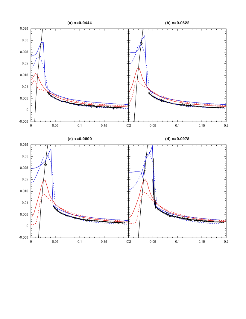
Figure 3: Flow near bow.

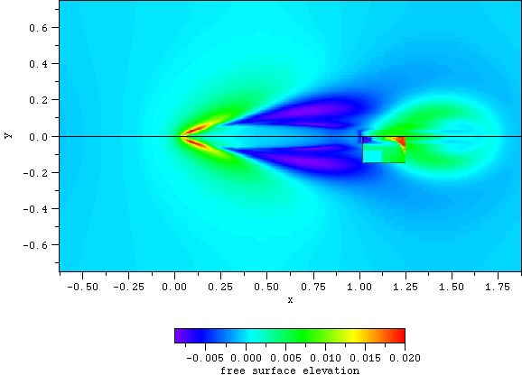
Figure 4: Flow near stern.

Figures 3 and 4 compare measurements at the bow and stern to the numerical predictions. The bow measurements include profile and whisker-probe measurements. Comparisons to the bow data are performed at four stations: $x=0.0444$, $x=0.0622$, $x=0.0800$, and $x=0.0978$. The circular symbol denotes profile measurements. The solid black lines denote the outline of the hull and the whisker-probe measurements. The solid blue line is medium CLS and the dashed blue line is coarse CLS. The solid red line is medium level-set and the dashed red line is coarse level-set. In general, the CLS technique captures the rapid rise up the side of the hull. The level-set technique does less well in this regard. In the outer-flow region the CLS coarse results are slightly better than the CLS fine results. This may be attributed to the shallow depth that is used in the CLS. The level-set results appear to converge better in the outer-flow region, but the results of the fine simulation are required for confirmation.

Figure 4 shows the entire flow around the ship for the medium resolution level-set simulation. The stern whisker-probe measurements are overlaid for the purposes of comparison. Although the numerical results are not stationary, the shape of the stern contours show general agreement with laboratory measurements. However, the amplitude of the numerical results are significantly lower than the measurements. Note that the stern is partially dry in the numerical simulations. The outline of the hull is visible in the numerical simulations because the level-set function intersects the hull.

6.2 Spray Sheet Results

The Navier-Stokes equations in combination with a level-set formulation are used to study the breakup of two-dimensional sheet of water. The sheet is $l_{o}=6$mm thick. The length of the sheet is 24mm. The top and bottom of the sheet are bounded by air. The initial mean-velocity of the water is $u_{o}=3$m/s. The initial rms turbulent velocity of the water is $\tilde{u}=1.2$m/s. The air is initially quiescent. Based on the sheet thickness ($l_{o}$) and the mean velocity ($u_{o}$), the Reynolds number is $R_{e}=u_{o}l_{o}/\mu=18,000$ and the Weber number is $W_{e}=\rho u_{o}^{2}l_{o}/\sigma=730$, where $\mu$ is the kinematic viscosity of water, $\rho$ is the water density, and $\sigma$ is the surface tension. The density and viscosity ratios are $\lambda=\rho_{g}/\rho_{\ell}=0.0012$ and $\eta=\mu_{g}/\mu_{\ell}=0.018$, which are appropriate for air-water interfaces. This parameter regime roughly corresponds to experiments that were performed by Sarpkaya and Merrill (1998), [14]. Numerical convergence is established using $2048^{2}$ and $4096^{2}$ grid points. Second-order accuracy in space is established. A third-order Runge-Kutta scheme is used to integrate the system of equations with respect to time. Mass is conserved to within 0.25% throughout the entire calculation.

Figure 5 illustrates the evolution of a two-dimensional spray sheet. The black contour lines indicate the interface between air and water. The water sheet is bounded by air both at the top and the bottom of the sheet. The color contours denote the vorticity. The flow is turbulent within the water sheet and laminar in the air. The mean velocity and rms velocity profiles are initially top-hat functions. The flow is moving from left to right. The turbulent fluctuations in the water are initially immersed below the top of the sheet and above the bottom of the sheet (see Fig. 5:$\,t=0$).

The turbulence in the water diffuses and interacts with the interfaces (see Fig. 5:$\,t=2.5$). The initial interaction is a roughening of the air-water interface. A thin boundary layer forms in the air. The boundary layer is colored blue (negative) at the top of the sheet and colored red (positive) at the bottom of the sheet. As the interface gets rougher and ligaments begin to form, the air separates from the back of the ligaments. The boundary layer thickens, and air is dragged along the top and the bottoms of the sheet.

Primary vortex shedding initially occurs behind the ligaments (see lower left of sheet in Fig. 5:$\,t=5$). As the primary vortices are shed, their interactions lead to the formation of secondary and tertiary vorticity (see upper middle of sheet in Fig. 5:$\,t=7.5$). Vortices are periodically shed from the backs of ligaments (see lower middle of sheet in Fig. 5:$\,t=10$). There is evidence of vortex merging both in the air and in the water (see upper left of Fig. 5:$\,t=17.5$). Although there is significant flow separation in the air, there is little or no separation in the water. The largest ligaments are formed by eddies impinging on the interface (see upper left of Fig. 5:$\,t=12.5$). Cavities form in regions where primary vortices are trapped. The inlets to the cavities shed secondary vorticity, which tends to make the cavities even larger (see middle of sheet in Fig. 5:$\,t=15$). At the inlets to the cavities, vortex pairs are formed. Under their own self-induced velocities, the vortex pairs move into the cavities where they diffuse.

Note that droplets do not actually form at the tips of the ligaments because 2d flows are not subject to the same instabilities as 3d flows. The turbulent kinetic energy tends to concentrate in the thicker portions of the deformed spray sheet. The flow within the ligaments is relatively benign. In agreement with theory, the pressure at the tips of the longest ligaments roughly scales like $P=(W_{e}r)^{-1}$, where $r$ is the radius of curvature of the tip.

7 Conclusion

In this paper, we have outlined the key numerical algorithms for simulating free-surface flows on cartesian grids using level-set and coupled level-set and volume-of-fluid techniques. Preliminary numerical results have been shown for ship waves and spray sheets. The ship wave results indicate that cartesian-grid methods are capable of resolving the flow around a ship if the grid resolution is sufficient. Near the bow and stern, we estimate that the grid spacing along all three cartesian axes should be $\Delta=0.0005$ (based on ship length) in order to resolve breaking waves. On a parallel computer, it is possible to approach this level of grid resolution, but adaptive gridding may also be required to fully resolve the entire flow around a ship [15]. Alternatively, cartesian-grid methods could be embedded in more conventional boundary-fitted methods to capture complex flows near the bow or stern. The spray-sheet results show that cartesian-grid methods are capable of resolving the air and water boundary layer at realistic Reynolds numbers.

Acknowledgments. The first author is supported in part by NSF Division of Mathematical Sciences under award number DMS 9996349. The second author is supported by ONR under contract number N00014-97-C-0345. Dr. Edwin P. Rood is the program manager. The numerical simulations have been performed on the T3E computer at the Naval Oceanographic Office using funding provided by a Department of Defense Challenge Project. We are very grateful to Mr. George Innis, Dr. James Rottman, and Mr. Andrew Talcott for assistance with this paper.

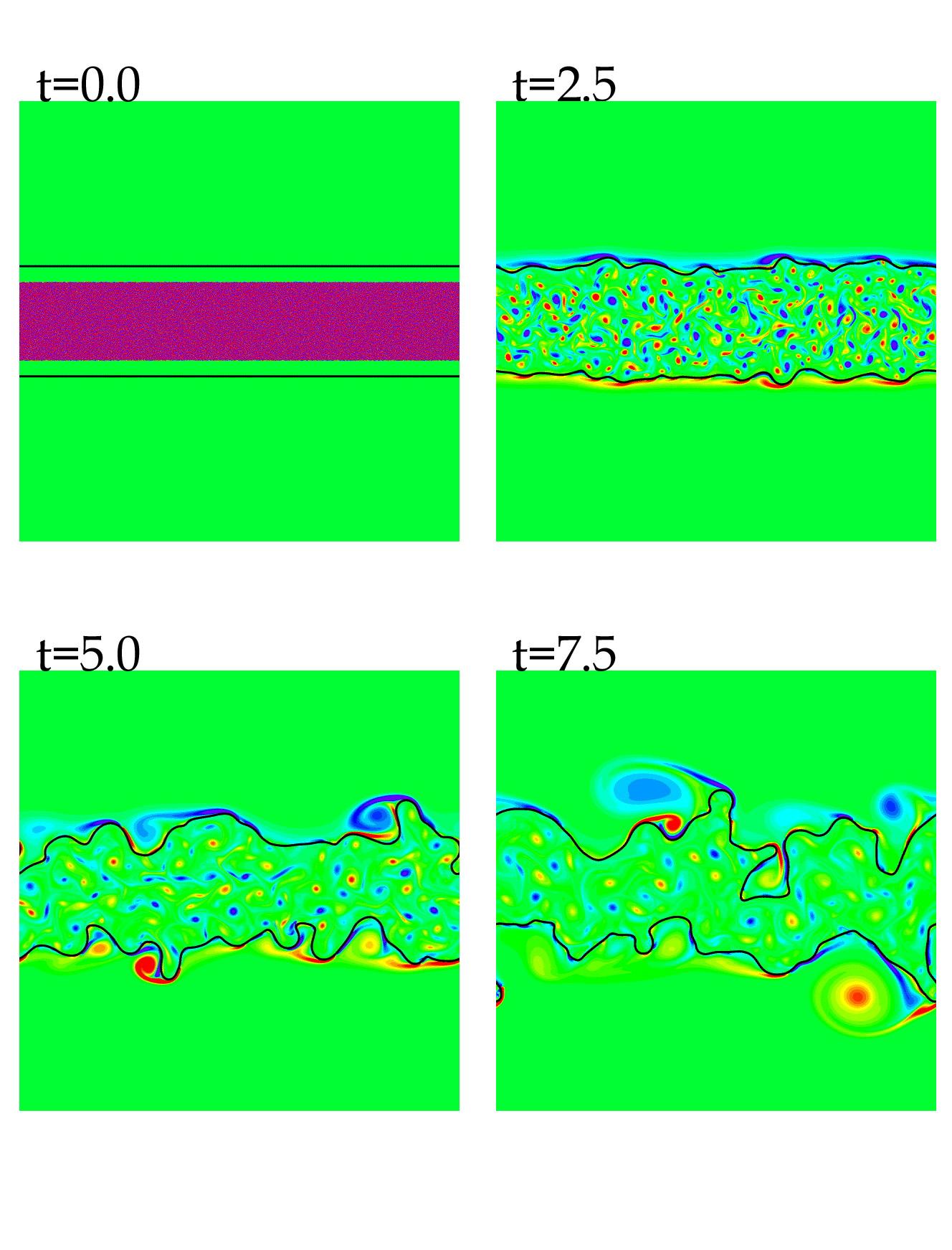
Figure 5: 2d spray sheet.

Figure 5: 2d spray sheet continued.

References

- [1] A. S. Almgren, J. B. Bell, P. Colella, and T. Marthaler. A cartesian grid projection method for the incompressible euler equations in complex geometries. SIAM J. Sci. Comput., 18(5):1289–1309, 1997.
- [2] J. B. Bell, P. Colella, and H. M. Glaz. A second-order projection method for the incompressible Navier-Stokes equations. J. Comput. Phys., 85:257–283, December 1989.
- [3] J. U. Brackbill, D. B. Kothe, and C. Zemach. A continuum method for modeling surface tension. J. Comput. Phys., 100:335–353, 1992.
- [4] Y.C. Chang, T.Y. Hou, B. Merriman, and S. Osher. Eulerian capturing methods based on a level set formulation for incompressible fluid interfaces. J. Comput. Phys., 124:449–464, 1996.
- [5] P. Colella, D.T. Graves, D. Modiano, E.G. Puckett, and M. Sussman. An embedded boundary/volume of fluid method for free surface flows in irregular geometries. In proceedings of the 3rd ASME/JSME joint fluids engineering conference, number FEDSM99-7108, San Francisco, CA, 1999.
- [6] R.G. Cox. The dynamics of the spreading of liquids on a solid surface. part 1. viscous flow. J. Fluid Mech., 168:169–194, 1986.
- [7] D.G. Dommermuth. Numerical Flow Analysis (nfa) working papers. Technical report, Science Applications International Corporation, 2000.
- [8] D.G. Dommermuth, G.E. Innis, T. Luth, E.A. Novikov, E. Schlageter, and J.C. Talcott. Numerical simulation of bow waves. In proceedings of the Twenty Second Symposium on Naval Hydro., pages 508–521, Washington, D.C., 1998.
- [9] L.M. Hocking and A.D. Rivers. The spreading of a drop by capillary action. J. Fluid Mech., 121:425–442, 1982.
- [10] H. Lamb. Hydrodynamics. Dover Publications, New York, 1932.
- [11] B. J. Leonard. Bounded higher-order upwind multidimensional finite-volume convection-diffusion algorithms. In W.J. Minkowycz and E.M. Sparrow, editors, Advances in Numerical Heat Transfer, volume I, pages 1–58. Taylor & Francis, 1997.
- [12] C.G. Ngan and E.B. Dussan V. On the dynamics of liquid spreading on solid surfaces. J. Fluid Mech., 209:191–226, 1989.
- [13] S. Osher and J. A. Sethian. Fronts propagating with curvature-dependent speed: Algorithms based on hamilton-jacobi formulations. J. Comput. Phys., 79(1):12–49, 1988.
- [14] T. Sarpkaya and C. Merrill. Spray formation at the free surface of liquid wall jets. In proceedings of the Twenty Second Symposium on Naval Hydro., pages 796–808, Washington, D.C., 1998.
- [15] M. Sussman, A. Almgren, J. Bell, P. Colella, L. Howell, and M. Welcome. An adaptive level set approach for incompressible two-phase flows. J. Comput. Phys., 148:81–124, 1999.
- [16] M. Sussman and E.G. Puckett. A coupled level set and volume of fluid method for computing 3d and axisymmetric incompressible two-phase flows. J. Comp. Phys. accepted for publication.
- [17] M. Sussman, P. Smereka, and S.J. Osher. A level set approach for computing solutions to incompressible two-phase flow. J. Comput. Phys., 114:146–159, 1994.
- [18] M. Sussman and S. Uto. Computing oil spreading underneath a sheet of ice. Technical Report CAM Report 98-32, University of California, Los Angeles, July 1998.
- [19] H.S. Udaykumar, H.C Kan, W. Shyy, and R. Tran-Son-Tay. Multiphase dynamics in arbitrary geometries on fixed cartesian grids. J. Comput. Phys., 137(2):366–405, 1997.