Energy Efficient Spectrum Sensing for State Estimation over A Wireless Channel

Abstract

The performance of remote estimation over wireless channel is strongly affected by sensor data losses due to interference. Although the impact of interference can be alleviated by performing spectrum sensing and then transmitting only when the channel is clear, the introduction of spectrum sensing also incurs extra energy expenditure. In this paper, we investigate the problem of energy efficient spectrum sensing for state estimation of a general linear dynamic system, and formulate an optimization problem which minimizes the total sensor energy consumption while guaranteeing a desired level of estimation performance. The optimal solution is evaluated through both analytical and simulation results.

I Introduction

Estimating the state of dynamic processes is a fundamental task in many real-time applications such as environment monitoring, health-care, smart grid, industrial automation and wireless network operations [1, 2]. Consider remotely estimating the state of a general linear dynamic system, where sensor data are transmitted over a wireless channel to a remote estimator. Due to interference from other users on the same channel, the sensor data may randomly get lost, which can significantly affect the estimation performance [3, 4, 5].

To alleviate the impact of interference, a sensor can adopt the “listen before talk” strategy, i.e., it can sense the channel first and only transmit data when the channel is clear. With spectrum sensing, the problem of estimation stability has been studied in [6, 7], and the questions of whether and to what extent the state estimation performance can be improved have been addressed in [7]. However, since both data transmission and spectrum sensing are energy consuming, the system energy efficiency becomes an important while challenging issue, which has not been studied in the literature yet.

In this paper, we investigate the problem of energy efficient spectrum sensing for state estimation over a wireless channel. Specifically, we consider when and how long to perform spectrum sensing in order to minimize the sensor’s total energy consumption while guaranteeing a certain level of estimation performance. The problem is modeled as a mixed integer nonlinear programming (MINLP) which jointly optimizes the spectrum sensing frequency and sensing time, subjecting to an estimation performance constraint. The joint optimization in fact achieves a balance between spectrum sensing and transmission energy consumption. We derive a condition under which the estimation error covariance is stable in mean sense. Since the mean estimation error covariance is usually a random value and may vary slightly but not converge along time, we resort to a close approximation of the constraint which results in an approximated optimization problem whose solution suffices the original problem. Finally, we provide both analytical and simulation results of the solution to the optimization problem. The remainder of the paper is organized as follows. Section II presents system model and optimization problem. The approximation problem is then introduced and analyzed in Section III. Section IV presents some simulation results, and Section V concludes this paper.

II System Model and Problem Setup

We consider estimating the state of a general linear discrete-time dynamic process as follows.

$$\left\{\begin{array}[]{lcl}x_{k+1}&=&Ax_{k}+w_{k},\\ y_{k}&=&Cx_{k}+v_{k},\end{array}\right.$$ (3)

where $x\in\mathbb{R}^{q_{1}}$ is the dynamic process state (e.g., environment variable) which changes along time. A wireless sensor is deployed to measure the process state and report the measurement to a remote estimator, where the sensor’s measurement about $x$ is $y\in\mathbb{R}^{q_{2}}$. In the above, $q_{1}$ and $q_{2}$ are dimensions of $x$ and $y$, respectively. Note that the estimator only has noisy information of both process model and sensor measurements. The noises are denoted as $w_{k}$ and $v_{k}$ with $\mathbb{E}[w_{k}w^{T}_{k}]=Q$, $\mathbb{E}[v_{k}v^{T}_{k}]=R$ and $\mathbb{E}[w_{i}v^{T}_{j}]=0$, where $(\cdot)^{T}$ denotes the transpose of a matrix or vector. $A$ and $C$ are constant matrices. Assume that $C$ has full column rank and that $(A,Q^{\frac{1}{2}})$ is controllable [3].

The sensor data are transmitted to a remote estimator where the transmissions are augmented by the spectrum sensing technique. The estimator applies a modified Kalman Filter [3] to estimate the system state $x$ recursively. Given the system model as shown in (3), define $\hat{x}_{k|k-1}$ and $\hat{x}_{k|k}$ as the prediction and estimate of the system state at step $k$, respectively. Define $P_{k|k-1}:=\mathbb{E}[(x_{k}-\hat{x}_{k|k-1})(x_{k}-\hat{x}_{k|k-1})^{T}]$ and $P_{k|k}:=\mathbb{E}[(x_{k}-\hat{x}_{k|k})(x_{k}-\hat{x}_{k|k})^{T}]$ as the covariance of the prediction and estimation errors, respectively. According to [3], the estimation process can be given as follows.

$$\left\{\begin{array}[]{rcl}\hat{x}_{k|k-1}&=&A\hat{x}_{k-1|k-1}\\ P_{k|k-1}&=&AP_{k-1|k-1}A^{T}+Q\\ \hat{x}_{k|k}&=&\hat{x}_{k|k-1}+\gamma_{k}K_{k}(y_{k}-C\hat{x}_{k|k-1})\\ K_{k}&:=&P_{k|k-1}C^{T}(CP_{k|k-1}C^{T}+R)^{-1}\\ P_{k|k}&=&(I-\gamma_{k}K_{k})P_{k|k-1}\end{array}\right.$$ (4)

with a given initial value $P_{1|0}\geq 0$, where $I$ is an identity matrix of compatible dimension. In the above, $\gamma_{k}\in\{0,1\}$ represents whether the measurement packet is dropped or not in step $k$, i.e., $\gamma_{k}=1$ if successfully received and $\gamma_{k}=0$ otherwise. $\mathbb{P}[\gamma_{k}=0]$ characterizes the packet loss rate.

Let $t_{I}$ and $t_{B}$ represent the idle and busy periods of the channel, respectively. We assume that [8]

$$\Gamma_{I}(t) =1-e^{-\alpha t}\textrm{~{}and~{}}\Gamma_{B}(t)=1-e^{-\beta t}.$$

Thus, $\mathbb{E}[t_{B}]=\frac{1}{\beta}$, $\mathbb{E}[t_{I}]=\frac{1}{\alpha}$ and the idle and busy probabilities are $p_{I}=\frac{\beta}{\alpha+\beta}$ and $p_{B}=\frac{\alpha}{\alpha+\beta}$, respectively. Define $\eta$ as the probability that the channel will keep idle for at least $t_{x}$ period of time conditioned on that it is currently idle. We have

$$\eta=\frac{1}{p_{I}}\int^{0}_{-\infty}\mathbb{P}[\textrm{an idle period begins}]\left[1-\Gamma_{I}(t_{x}-t)\right]dt$$

$$=\frac{1}{p_{I}}\int^{\infty}_{0}\frac{1}{\frac{1}{\alpha}+\frac{1}{\beta}}\left[1-\Gamma_{I}(t_{x}+t)\right]dt$$

$$=\alpha\int^{\infty}_{0}e^{-\alpha(t_{x}+t)}dt=e^{-\alpha t_{x}}.$$

We assume that the sensing time $\tau$ is bounded within $[0,\bar{\tau}]$ and is much smaller than both $\mathbb{E}[t_{B}]$ and $\mathbb{E}[t_{I}]$. Therefore, the channel state does not change during spectrum sensing (almost surely), and henceforth we can treat the sensing period as a point in time. The sampling period $T_{s}\gg\max(\mathbb{E}[t_{B}],\mathbb{E}[t_{I}])$, so that the packet drop rate in the current sampling period is irrelevant with that in previous steps. Based on this, the measurement packet drop rate, i.e., $\mathbb{P}[\gamma_{k}=0]$, also can be deemed time-independent.

Before transmitting a packet, the sensor must check the channel state and transmit packet only when the channel is available (in idle state). We adopt the energy detection [8] as our spectrum sensing method. Let $s_{c}$ be the sensing outcome and define following two probabilities.

$$p_{d}=\; \mathbb{P}[s_{c}=\textrm{`idle'}|\textrm{channel is idle}]$$

$$=\; Q\left((1-\epsilon_{d})\sqrt{\tau W}\right),$$ (5)

$$p_{f}=\; \mathbb{P}[s_{c}=\textrm{`idle'}|\textrm{channel is busy}]$$

$$=\; Q\left((1-{\epsilon_{f}})\sqrt{\tau W}\right),$$ (6)

where $\epsilon_{d}>\epsilon_{f}>0$, $W$ is the channel bandwidth, and $Q(z):=\frac{1}{\sqrt{2\pi}}\int^{\infty}_{z}e^{-\frac{\tau^{2}}{2}}d\tau$. In the following, $p_{d}$ and $p_{f}$ are called the correct and false detection probabilities, respectively.

After sensing, the sensor will transmit packet only if the sensing result indicates an idle channel (we call this event a successful sensing). Thus, the transmission probability is

$$p_{tx} =p_{I}p_{d}+p_{B}p_{f}=\frac{1}{\alpha+\beta}(\beta p_{d}+\alpha p_{f}).$$ (7)

Define a sequence of variables $\{\theta_{k}\in\{0,1\}\}_{k\geq 1}$ as

$$\theta_{k}=\left\{\begin{array}[]{rl}1,&\textrm{sense the channel in step $k$,}\\ 0,&\textrm{otherwise}.\end{array}\right.$$ (8)

Let $\Theta:=\{k|\theta_{k}=1\}$, which is called the spectrum sensing schedule. In this paper, we restrict our attention to strict periodical spectrum sensing, i.e., $\Theta=\Theta_{n}:=\{0,n,2n,\ldots\}=\{k_{i}|k_{i}=in,i\in\mathbb{N}^{+}\cup\{0\}\}$, where $n$ represents the reciprocal of the sensing frequency.

II-A Problem Formulation

Let $e_{s}$ and $e_{tx}$ denote the amounts of energy consumed by the sensor for conducting spectrum sensing in a unit time and transmitting a measurement packet (assume all packets are of the same length), respectively. If $\theta_{k}=1$, the average amount of energy consumed by the sensor in $k$th step is $\varphi_{s}=\tau e_{s}+p_{tx}e_{tx}$. Therefore, under schedule $\Theta_{n}$, the average energy consumption in a single step is

$$\bar{\varphi}=\frac{1}{n}\varphi_{s}=\frac{1}{n}(\tau e_{s}+p_{tx}e_{tx}).$$ (9)

The estimation performance can be characterizes by the error covariance $P_{k|k-1}$. For ease of exposition, hereafter, we let $P_{k}:=P_{k|k-1}$. Based on the estimation process above, we can see that $P_{k}$ is a function of the random variable $\gamma_{k}$; hence it is both random and time-varying and may not converge along an infinite horizon. Therefore, we consider the long-time average of the expected $P_{k}$, i.e., $\frac{1}{L}\sum^{L}_{k=1}\mathbb{E}[P_{k}]$, where $L$ is a sufficiently large number. We aim to bound this average value below a user defined threshold $\bar{P}$. With this constraint, our optimization problem can be formulated as follows.

Problem 1

Find the optimal schedule $\Theta_{n}$ and spectrum sensing time $\tau$ to

$$\left\{\begin{array}[]{rl}\min\limits_{n,\tau}&\;\bar{\varphi}=\frac{1}{n}(\tau e_{s}+p_{tx}e_{tx})\\ s.t.&\;\frac{1}{L}\sum^{L}_{k=1}\mathbb{E}[P_{k}]\leq\bar{P}\\ &\;0\leq\tau\leq\bar{\tau}.\end{array}\right.$$ (10)

As can be seen, Problem 1 is a mixed integer nonlinear programming. Note that, through the joint optimization, the sensing energy and transmission energy are balanced.

III Main Results

III-A Estimation Stability

To satisfy the constraints in (10), the sequence $\{\mathbb{E}[P_{k}]\}$ must be stable, i.e., $\mathbb{E}[P_{k}]<\infty,\forall k\geq 1$. For any $k\geq 1$, if $\theta_{k}=1$, based on the estimation process above, we have

$$P_{k}=\; AP_{k-1}A^{T}+Q$$

$$-\gamma_{k}AP_{k-1}C^{T}(CP_{k-1}C^{T}+R)^{-1}CP_{k-1}A^{T}$$

$$=\; (1-\gamma_{k})AP_{k-1}A^{T}+Q$$

$$+\gamma_{k}A(P^{-1}_{k-1}+C^{T}R^{-1}C)^{-1}A^{T}$$

$$=\; (1-\gamma_{k})AP_{k-1}A^{T}+Q+\gamma_{k}A\Upsilon_{k-1}A^{T},$$ (11)

where $\Upsilon_{k-1}=(P^{-1}_{k-1}+C^{T}R^{-1}C)^{-1}$ is upper-bounded by $(C^{T}R^{-1}C)^{-1}$ (notice that $C$ has full column rank) [7].

Otherwise, $\theta_{k}=0$, which is similar to the case that the measurement packet gets lost. Then, $P_{k}=AP_{k-1}A^{T}+Q$. Consider the schedule $\Theta_{n}$. We have

$$P_{k_{i}-1}=\; AP_{k_{i}-2}A^{T}+Q=\ldots$$

$$=\; A^{n-1}P_{k_{i-1}}(A^{T})^{n-1}+\sum^{n-2}_{t=0}A^{t}Q(A^{T})^{t}.$$ (12)

Substituting the above equation into (III-A) yields

$$P_{k_{i}}=\; (1-\gamma_{k_{i}})A^{n}P_{k_{i-1}}(A^{T})^{n}+(1-\gamma_{k_{i}})\sum^{n-1}_{t=1}A^{t}Q(A^{T})^{t}$$

$$+Q+\gamma_{k_{i}}A\Upsilon_{k_{i}-1}A^{T},$$ (13)

$$\mathbb{E}[P_{k_{i}}]=\; (1-\gamma)A^{n}\mathbb{E}[P_{k_{i-1}}](A^{T})^{n}+(1-\gamma)\sum^{n-1}_{t=1}A^{t}Q(A^{T})^{t}$$

$$+Q+\gamma A\mathbb{E}[\Upsilon_{k_{i}-1}]A^{T},$$ (14)

where $\gamma$ is the successful packet reception rate under $\theta_{k}=1$, which can be calculated by

$$\gamma =\mathbb{P}[\gamma_{k}=1|\theta_{k}=1,s_{c,k}=\textrm{`idle'}]$$

$$=p_{I}\eta p_{d}=\frac{\beta}{\alpha+\beta}p_{d}e^{-\alpha t_{x}},$$ (15)

where $s_{c,k}$ is the spectrum sensing result. Since $n$ is a finite constant, the stability of $\{\mathbb{E}[P_{k}]\}$ is equivalent to that of the original sequence $\{\mathbb{E}[P_{k_{i}}]\}$. Moreover, since $\Upsilon_{k_{i}-1}$ is bounded by a constant, the stability of $\{\mathbb{E}[P_{k_{i}}]\}$ is further equivalent to that of $\{X_{k_{i}}|X_{k_{i}}=(1-\gamma)A^{n}X_{k_{i-1}}(A^{T})^{n}+\sum^{n-1}_{t=0}A^{t}Q(A^{T})^{t}\}$. Therefore, it is easy to obtain the following condition which is both necessary and sufficient for the stability of $\{\mathbb{E}[P_{k}]\}$.

Theorem 1

$\forall\ n\geq 1$, $\{\mathbb{E}[P_{k}]\}$ is stable if and only if

$$(1-\gamma)\lambda_{\max}^{2n}(A)<1,$$ (16)

where $\lambda_{\max}(\cdot)$ is the maximum eigenvalue of a square matrix.

Since $p_{d}\leq 1$, (III-A) indicates that $\gamma\leq\frac{\beta}{\alpha+\beta}e^{-\alpha t_{x}}<\frac{\beta}{\alpha+\beta}$. Therefore, an upper bound of $n$ can be obtained based on (16) as follows.

$$n\leq\bar{n}_{1}=\left\{\begin{array}[]{ll}\lceil\frac{\ln(\alpha+\beta)-\ln\alpha}{2\ln(\lambda_{\max}(A))}\rceil-1,&\textrm{ if }\lambda_{\max}(A)>1\\ \infty,&\textrm{ otherwise}.\end{array}\right.$$ (17)

III-B Problem Approximation

As shown in (III-A), since $P_{k-1}$ appears in the inverse term of $\Upsilon_{k-1}$, $\mathbb{E}[P_{k}]$ will depend on all possible values of the sequence $\{\gamma_{k}\}_{k\geq 1}$. Moreover, $\mathbb{E}[P_{k}]$ may not necessarily converge. As a result, it is mathematically difficult to obtain the long-term average of $\mathbb{E}[P_{k}]$. Therefore, we resort to an upper bound of $\mathbb{E}[P_{k}]$ to sufficiently satisfy the constraint in Problem 1. Based on Theorem 4 in [3], we have

$$\mathbb{E}[P_{k}]=\; \mathbb{E}[-\gamma_{k}AP_{k-1}C^{T}(CP_{k-1}C^{T}+R)^{-1}CP_{k-1}A^{T}]$$

$$+\mathbb{E}[AP_{k-1}A^{T}+Q]$$

$$\leq -\gamma A\mathbb{E}[P_{k-1}]C^{T}(C\mathbb{E}[P_{k-1}]C^{T}+R)^{-1}C\mathbb{E}[P_{k-1}]A^{T}$$

$$+A\mathbb{E}[P_{k-1}]A^{T}+Q.$$ (18)

Define a sequence $\{Y_{k}\}$ with

$$Y_{k}=\; AY_{k-1}A^{T}+Q$$

$$-\theta_{k}\gamma AY_{k-1}C^{T}(CY_{k-1}C^{T}+R)^{-1}CY_{k-1}A^{T}.$$ (19)

Then, $\mathbb{E}[P_{k}]\leq Y_{k}$ if we let $Y_{0}=P_{0}$. Lemma 1 characterizes the sequence $\{Y_{k}\}$; its proof is omitted due to limited space.

Lemma 1

If (16) holds, $\exists\bar{Y}(\gamma,n)>0$ such that

$$\lim_{L\to\infty}\frac{1}{L}\sum^{L}_{k=1}Y_{k}=\bar{Y}(\gamma,n).$$ (20)

$\bar{Y}(\gamma,n)$ is monotonically decreasing as either $\gamma$ increases or $n$ decreases. Furthermore, for a sufficiently large $L$,

$$\frac{1}{L}\sum^{L}_{k=1}\mathbb{E}[P_{k}]\leq\frac{1}{L}\sum^{L}_{k=1}Y_{k}\rightarrow\bar{Y}.$$ (21)

Based on Lemma 1, the constraint in Problem 1 can be approximated as $\bar{Y}(\gamma,n)\leq\bar{P}$. Due to the monotonicity of $\bar{Y}(\gamma,n)$ in $\gamma$, it is equivalent to say that $\gamma\geq\underline{\gamma}(n)$ where $\underline{\gamma}(n)$ is the unique solution of $\gamma$ to $\bar{Y}(\gamma,n)=\bar{P}$. On the other hand, since $\gamma\leq\frac{\beta}{\alpha+\beta}e^{-\alpha t_{x}}$, the inequality $\bar{Y}(\frac{\beta}{\alpha+\beta}e^{-\alpha t_{x}},n)\leq\bar{Y}(\gamma,n)\leq\bar{P}$ yields another upper bound on $n$:

$$n\leq\bar{n}_{2}=\max\left\{\tilde{n}\bigl{|}\bar{Y}\left(\frac{\beta}{\alpha+\beta}e^{-\alpha t_{x}},\tilde{n}\right)\leq\bar{P}\right\}<\infty.$$ (22)

Therefore, we get an approximation of Problem 1 as below.

Problem 2

Find the optimal schedule $\Theta_{n}$ and spectrum sensing time $\tau$ to

$$\left\{\begin{array}[]{rl}\min\limits_{\Theta_{n},\tau}&\;\bar{\varphi}=\frac{1}{n}(\tau e_{s}+p_{tx}e_{tx})\\ s.t.&\;\gamma\geq\underline{\gamma}(n)\\ &\;n\leq\bar{n}=\min\{\bar{n}_{1},\bar{n}_{2}\}\\ &\;0\leq\tau\leq\bar{\tau}.\end{array}\right.$$ (27)

III-C Optimal Solution Analysis

Given any $n$, Problem 2 reduces to a subproblem with $\tau$ as the only decision variable. Since $n<\bar{n}$, the optimal $n^{*}$ and $\tau^{*}$ can be obtained by solving $\bar{n}$ such subproblems. In the following, we analyze the optimal solution $\tau^{*}_{n}$ under any given $n$. Let $\rho=\frac{\alpha}{\beta}$. We focus on that $\rho<1$, while the case that $\rho\geq 1$ can be analyzed in the same way. For ease of analysis, we assume $\tau$ is continuous. Given $n$, the subproblem has following properties.

$$\frac{\partial\gamma}{\partial\tau}=\; \frac{(1-p_{1})\sqrt{W}}{2\sqrt{2\pi\tau}}(\epsilon_{d}-1)e^{-\frac{(1-\epsilon_{d})^{2}}{2}W\tau}$$ (28)

$$\frac{\partial\bar{\varphi}}{\partial\tau}=\; \frac{1}{n}\left(e_{s}+\frac{e_{tx}\sqrt{W}}{2(1+\rho)\sqrt{2\pi\tau}}f(\epsilon_{d},\epsilon_{f},\tau)\right)$$ (29)

$$f(\epsilon_{d},\epsilon_{f},\tau)\triangleq (\epsilon_{d}-1)e^{-\frac{(1-\epsilon_{d})^{2}}{2}W\tau}$$

$$-\rho(1-\epsilon_{f})e^{-\frac{(1-\epsilon_{f})^{2}}{2}W\tau}.$$ (30)

Depending on the values of $\epsilon_{d}$ and $\epsilon_{f}$ (note that $\epsilon_{f}<\epsilon_{d}$), the shapes of the $\gamma$ and $\bar{\varphi}$ curves are described as follows.

1) If either $\epsilon_{d}\geq 1$ and $\epsilon_{f}\geq 1$ or $\rho\leq\frac{\epsilon_{d}-1}{1-\epsilon_{f}}\leq 1$ and $\epsilon_{f}<1$, it is easy to see that $\frac{\partial\gamma}{\partial\tau}\geq 0$ and $\frac{\partial\bar{\varphi}}{\partial\tau}\geq 0$, which means that both $\gamma$ and $\bar{\varphi}$ are increasing as $\tau$ increases. This corresponds to case 1 as shown in Fig. 1(a).

2) If $\frac{\epsilon_{d}-1}{1-\epsilon_{f}}>1$ and $\epsilon_{f}<1$, since $e^{-\frac{(1-\epsilon_{d})^{2}}{2}W\tau}<e^{-\frac{(1-\epsilon_{f})^{2}}{2}W\tau}$, $f(\epsilon_{d},\epsilon_{f},\tau)$ varies from positive infinite to a negative value and finally converges to 0. Depending on the parameters such as $e_{s}$ and $e_{tx}$, the shape of $\bar{\varphi}$ will be in the form of either case 1 or case 2 as shown in Fig. 1(b).

3) If $0\leq\epsilon_{d}-1<\rho(1-\epsilon_{f})$, one can verify that $\frac{\partial^{2}}{\partial^{2}\tau}f(\epsilon_{d},\epsilon_{f},\tau)>0$; hence, $\frac{\partial\bar{\varphi}}{\partial\tau}$ increases from negative infinite to a positive value. Therefore, as shown in Fig. 1(c), $\bar{\varphi}$ is a convex function.

4) Otherwise, $\epsilon_{d}<1$. Then, $\epsilon_{f}<1$ either. Consequently, $\frac{\partial\gamma}{\partial\tau}<0$ and $\frac{\partial}{\partial\tau}f(\epsilon_{d},\epsilon_{f},\tau)<0$. As shown in Fig. 1(d), the objective function is convex.

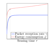
(a) Case 1

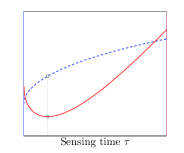
(b) Case 2

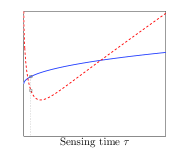
(c) Case 3

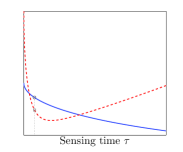
(d) Case 4

Figure 1: Illustrations of the optimal $\tau$ under different $\epsilon_{d}$ and $\epsilon_{f}$.

As shown in the figure, in case 1, the optimal $\tau^{*}_{n}$ is the smaller one between $\bar{\tau}$ and the point where $\gamma=\underline{\gamma}(n)$. In the other cases, let $\tau_{n,\bar{\varphi}}$ and $\tau_{n,\gamma}$ be the solution points for $\frac{\partial\bar{\varphi}}{\partial\tau}=0$ and $\gamma=\underline{\gamma}(n)$, respectively. In case 2, $\tau^{*}_{n}$ is among $\{0,\tau_{n,\bar{\varphi}},\tau_{n,\gamma},\bar{\tau}\}$. In the other cases, $\tau^{*}_{n}\in\{\tau_{n,\bar{\varphi}},\tau_{n,\gamma},\bar{\tau}\}$.

IV Simulation Results

In our simulations, we consider a linear system (3) with $A=\begin{bmatrix}1.05&0\\ 1&0.9\end{bmatrix}$, $C=I$, $Q=I$ and $R=0.8I$, where $I$ is the 2-by-2 identity matrix. The sensor samples the system every $T_{s}=1$ second and the transmission time of each measurement packet is $t_{x}=50ms$. The wireless channel has bandwidth $W=2Mbps$, noise power $\sigma_{n}=1$ and signal-to-noise ratio $-3dB$. The default average busy and idle rates for the channel are $\alpha=5$ and $\beta=20$, respectively. Other parameters are: $\epsilon_{d}=1.2$, $\bar{\tau}=20ms$, $e_{s}=e_{tx}=100$. The estimation performance requirement is set as $\bar{P}=\bar{Y}(0.7,6)$, where $\bar{Y}(\gamma,n)$ is defined in Lemma 1.

The optimal solutions of Problem 2 are depicted in Fig. 2. In the left figure, we vary the channel idle probability $p_{I}$ by gradually increasing $\beta$. The results show that, under a certain $n$, the optimal sensing time $\tau^{*}$ drops quickly as the idle probability increases, which in turn results in the decrease of the average energy consumption $\bar{\varphi}$. In fact, as the channel quality becomes better, less sensor energy will be wasted for conduction unsuccessful sensing and collided transmissions. Meanwhile, when $p_{I}$ increases from 0.3 to 1, the optimal $n$ increases piecewise, which means that the sensor conducts spectrum sensing and packet transmission less frequently. Therefore, generally speaking, the energy consumption decreases as $p_{I}$ increases.

The right figure demonstrate the optimal solutions under varying $e_{tx}/e_{s}$. As $e_{tx}$ increases, i.e., the transmission energy becomes to dominate the total energy $\bar{\varphi}$, the sensor’s best strategy becomes to transmit data less frequently but more reliably in order to avoid collision and save energy. Therefore, it will use a larger $n$ and spend more sensing time to increase the sensing accuracy, which are clearly shown in Fig. 2.

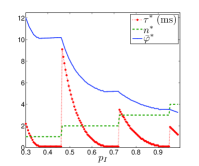
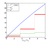
Figure 2: Optimal solutions under varying $p_{I}$ and $e_{tx}/e_{s}$.

V Conclusion

We have studied the energy efficient spectrum sensing problem for remote state estimation and formulated it as a mixed integer nonlinear programming problem. Both analytical and simulation results of the optimal solutions of the spectrum sensing time $\tau^{*}$ and period $n^{*}$ have been provided. We showed that, as $p_{I}$ increases, $n^{*}$ increases piecewise and the resulted energy consumption decreases. On the other hand, both $n^{*}$ and $\tau^{*}$ increase piecewise as $e_{tx}$ increases. Our future directions include extending the idea to multiple channel and multiple sensor scenarios.

References

- [1] J. Hespanha, P. Naghshtabrizi, and Y. Xu, “A survey of recent results in networked control systems,” Proceedings of the IEEE, vol. 95, no. 1, pp. 138–162, 2007.
- [2] R. T. Sukhavasi and B. Hassibi, “The kalman-like particle filter: Optimal estimation with quantized innovations/measurements,” IEEE Transactions on Signal Processing, vol. 61, no. 1, pp. 131–136, 2013.
- [3] B. Sinopoli, L. Schenato, M. Franceschetti, K. Poolla, M. Jordan, and S. Sastry, “Kalman filtering with intermittent observations,” IEEE Transactions on Automatic Control, vol. 49, no. 9, pp. 1453–1464, Sep. 2004.
- [4] M. Huang and S. Deyb, “Stability of kalman filtering with markovian packet losses,” Automatica, vol. 43, no. 4, pp. 598–607, 2007.
- [5] E. Rohr, D. Marelli, and M. Fu, “A unified framework for mean square stability of kalman filters with intermittent observations,” in Proc. IEEE International Conference on Control and Automation (ICCA), 2011, pp. 177–182.
- [6] X. Ma, S. M. Djouadi, and H. Li, “State estimation over a semi-markov model based cognitive radio system,” IEEE Transactions on Wireless Communications, vol. 11, no. 7, pp. 2391–2401, 2012.
- [7] X. Cao, P. Cheng, J. Chen, S. S. Ge, Y. Cheng, and Y. Sun, “Cognitive radio based state estimation in cyber-physical systems,” IEEE Journal on Selected Areas in Communications, vol. 32, no. 3, pp. 489–502, 2014.
- [8] W.-Y. Lee and I. Akyildiz, “Optimal spectrum sensing framework for cognitive radio networks,” IEEE Transactions on Wireless Communications, vol. 7, no. 10, pp. 3845–3857, Oct. 2008.