Turbulence-Induced Relative Velocity of Dust particles IV: the Collision Kernel

Abstract

Motivated by its importance for modeling dust particle growth in protoplanetary disks, we study turbulence-induced collision statistics of inertial particles as a function of the particle friction time, $\tau_{\rm p}$. We show that turbulent clustering significantly enhances the collision rate for particles of similar sizes with $\tau_{\rm p}$ corresponding to the inertial range of the flow. If the friction time, $\tau_{\rm p,h}$, of the larger particle is in the inertial range, the collision kernel per unit cross section increases with increasing friction time, $\tau_{\rm p,l}$, of the smaller particle, and reaches the maximum at $\tau_{\rm p,l}=\tau_{\rm p,h}$, where the clustering effect peaks. This feature is not captured by commonly-used kernel formula, which neglects the effect of clustering. We argue that turbulent clustering helps alleviate the bouncing barrier problem for planetesimal formation. We also investigate the collision velocity statistics using a collision-rate weighting factor to account for higher collision frequency for particle pairs with larger relative velocity. For $\tau_{\rm p,h}$ in the inertial range, the rms relative velocity with collision-rate weighting is found to be invariant with $\tau_{\rm p,l}$ and scales with $\tau_{\rm p,h}$ roughly as $\propto\tau_{\rm p,h}^{1/2}$. The weighting factor favors collisions with larger relative velocity, and including it leads to more destructive and less sticking collisions. We compare two collision kernel formulations based on spherical and cylindrical geometries. The two formulations give consistent results for the collision rate and the collision-rate weighted statistics, except that the spherical formulation predicts more head-on collisions than the cylindrical formulation.

1. Introduction

Modeling the growth of dust particles in turbulent protoplanetary disks is of crucial importance for understanding the challenging problem of planetesimal formation. While the classical picture for planetesimal formation by gravitational instability in a dense dust layer at the disk mid plane suffers from self-generated turbulence (see Chiang & Youdin 2010 for a review), the mechanism via the collisional growth of dust grains from (sub)micron size to kilometer size is frustrated by the meter-size barrier. As the particles grow to decimeter sizes, they become less sticky and, depending on the particle properties and the collision velocity, the collisions may result in bouncing or fragmentation (Blum & Wurm 2008; Güttler et al. 2010). This would suppress the further growth of the particles past the meter size. Meanwhile, the meter-size particles have large radial drift velocities and may rapidly get lost to the central star on a timescale of a hundred years (Weidenschilling 1977). The viability of planetesimal formation by dust coagulation depends on how fast and to which size dust particles can grow by collisions.

To answer this question, an accurate evaluation of the collision statistics is required. In a series of recent papers (Pan & Padoan 2013, Pan et al. 2014a, 2014b), we have investigated the statistics of the relative velocity of dust particles induced by turbulent motions. In Pan & Padoan (2013) and Pan et al.  (2014a), we conducted a systematic study of the root-mean-square (rms) of turbulence-induced relative velocity using both numerical and analytical approaches. In particular, we showed that the prediction of the Pan & Padoan (2010) model for the rms relative velocity is in good agreement with the simulation data, confirming the physical picture of the model. In Pan et al. (2014b), we analyzed the probability distribution of the relative velocity as a function of the particle friction time, and discussed its important role in determining the fractions of collisions leading to sticking, bouncing and fragmentation (Windmark et al. 2012, Garaud et al. 2013).

In this fourth paper, we focus on the turbulence-induced collision kernel, extending the earlier result on equal-size particles, known as the monodisperse case (Pan & Padoan 2013, hereafter Paper I), to the general bidisperse case for different particles of arbitrary sizes. The collision kernel is needed to estimate the collision rate of dust particles. Coagulation models for dust particles in protoplanetary disks set the kernel to be the product of the cross section and the root-mean-square (rms) relative velocity of the colliding particles. These studies commonly adopt the model of Völk et al. (1980) and its later developments for the rms collision velocity (e.g., Markiewicz et al. 1991, Cuzzi & Hogan 2003, Ormel & Cuzzi 2007). For convenience, we will refer to this type of models generally as the Völk-type model.

There are several uncertainties in the commonly-used prescriptions for dust particle collisions. First, the effect of turbulent clustering (Maxey 1987) on the collision kernel was typically not accounted for. Second, most theoretical models, including Völk et al. (1980) and our model (Pan & Padoan 2010), only predict the 2nd order moment (rms) of the relative velocity, while the calculations of the collision kernel and the average collision energy require the 1st and the 3rd oder moments respectively (e.g., Hubbard 2012, 2013). Finally, the accuracy of the Völk-type model and the kernel formulation have not been systematically tested against numerical simulations. An assessment of the Völk-type model is of particular interest, considering a weakness of its physical picture raised in our earlier works (Pan & Padoan 2010, 2013). In this paper, we will focus on evaluating the collision kernel and the collision velocity statistics using a numerical simulation and on clarifying the first two uncertainties in the commonly-used kernel formulation. We defer a thorough assessment of the accuracy of Völk-type models for the rms relative velocity to a later work.

In §2, we describe the simulation used in this work. §3 presents numerical results for the collision kernel, including the effects of turbulent clustering and turbulent-induced relative velocity. In §4, we analyze the collision velocity statistics weighted by the collision rate, which accounts for the higher collision frequency for particle pairs with larger relative velocity. §5 discusses the implication of our numerical results on dust particle growth in protoplanetary disks. Our conclusions are summarized in §6.

2. Numerical Simulation

We analyze the simulation data of Pan & Padoan (2013; hereafter Paper I). In the simulation, we evolved a weakly compressible flow on a uniform 512³ periodic grid and integrated the trajectories of inertial particles in a wide size range using the Pencil code (Brandenburg & Dobler 2002, Johansen et al. 2004). The turbulent flow was driven and maintained by a large-scale solenoidal force generated in Fourier space using all modes with wave length larger than half box size. The three components of each mode are independently drawn from Gaussian distributions of equal variance. The direction for each mode is random, and the driving force is statistically refreshed at each time step. This conventional driving scheme produces a turbulent flow with the broadest inertial range possible at a given resolution and the maximum degree of statistical isotropy. At steady state, the rms Mach number, $M$, of the simulated flow is $\simeq 0.1$, consistent with turbulence conditions in protoplanetary disks. There has been compelling evidence that the behavior of structure functions of all orders in a subsonic turbulent flow with $M\;\hbox to0.0pt{\lower 2.5pt\hbox{$\sim$}\hss}\raise 1.5pt\hbox{$<$}\;1$ is almost identical to incompressible turbulence (e.g., Porter et al. 2002, Padoan et al. 2004, Pan & Scannapieco 2011). This suggests that, at $M\;\hbox to0.0pt{\lower 2.5pt\hbox{$\sim$}\hss}\raise 1.5pt\hbox{$<$}\;1$, the particle collision statistics would be insensitive to the Mach number, and our results are applicable for any subsonic turbulent flow.

The regular and Taylor Reynolds numbers of the simulated flow are $\simeq 1000$ and $\simeq 200$, respectively. The 1D rms flow velocity is $u^{\prime}\simeq 6.8u_{\eta}$, with $u_{\eta}$ the Kolmogorov velocity. The integral scale, $L$, of the flow is about 1/6 of the box size, and the Kolmogorov scale is $\eta\simeq 0.6$ grid cell size. The large eddy time, $T_{\rm eddy}\equiv L/u^{\prime}$, was estimated to be $20\tau_{\eta}$, where $\tau_{\eta}$ is the Kolmogorov timescale, corresponding to the smallest eddies in the flow. Using tracer particles, we also measured the Lagrangian correlation time, $T_{\rm L}\simeq 14.4\tau_{\eta}$. As shown in Paper I, $T_{\rm L}$ is more relevant than $T_{\rm eddy}$ for understanding the particle velocity. We refer the reader to our earlier papers (Papers I & II) for a detailed description of the statistics of the simulated flow velocity field, ${\boldsymbol{u}}$.

In the simulated flow, we evolved 14 particle species of different sizes, each containing 33.6 million particles. The particle inertia is characterized by the friction or stopping time, $\tau_{\rm p}$, which ranges from $0.1\tau_{\eta}$ to $43\,T_{\rm L}$. Defining the Stokes number as $St\equiv\tau_{\rm p}/\tau_{\eta}$, this range corresponds to $0.1\leq St\leq 800$. We compute the relative velocity, ${\boldsymbol{w}}\equiv{\boldsymbol{v}}^{(1)}-{\boldsymbol{v}}^{(2)}$, of nearby particles (1) and (2) (with velocities ${\boldsymbol{v}}^{(1,2)}$) at a small separation, ${\boldsymbol{r}}$, and analyze the collision statistics as a function of the Stokes number pairs ($St_{1}$, $St_{2}$). We denote the Stokes numbers of the smaller and larger particles as $St_{\ell}$ and $St_{h}$, respectively. It is convenient to show the collision kernel and velocity as functions of the friction time, $\tau_{\rm ph}$ (or the Stokes number $St_{h}$) of the larger particle, and the friction time ratio $f$, defined as $f\equiv St_{\ell}/St_{h}$. By definition, $0\leq f\leq 1$. The method used to analyze the particle statistics was given in Paper I, to which we refer the reader for details.

An interesting question concerning our simulation is whether the particle collision statistics depends on the driving scheme adopted for the turbulent flow. Considering the universality of turbulent structures at small scales, we expect that the collisions of relatively small particles with $\tau_{\rm p}$ much below $T_{\rm eddy}$ (or $T_{\rm L}$) are not affected by the driving mechanism. The same is expected for the large particle limit with $\tau_{\rm p}\gg T_{\rm eddy}$. The motions of these large particles are similar to Brownian motion because even the largest eddies in the flow would act like random kicks, when viewed on the friction time, $\tau_{\rm p}$, of these particles. Therefore, collisions of particles in the $\tau_{\rm p}\gg T_{\rm eddy}$ limit are also insensitive to the details of the velocity structures at the driving scale. However, for intermediate particles with $\tau_{\rm p}$ close to $T_{\rm eddy}$, the dynamics is coupled to the flow velocity structures around the driving scale, which are non-universal, and thus their collision statistics may depend on how the flow is driven. An exploration of this possible dependence requires a number of numerical simulations using different driving schemes, which are computationally expensive and beyond the scope of the current work.

3. The Collision Kernel

The collision rate per unit volume between two particle species with Stokes numbers $St_{1}$ and $St_{2}$ can be expressed as $\bar{n}_{1}\bar{n}_{2}\Gamma$, where $\bar{n}_{1}$ and $\bar{n}_{2}$ are the average number densities and $\Gamma$ is the collision kernel (see Zhou et al. 2001). In Saffman & Turner (1956), two formulations, named the spherical and cylindrical formulations, were proposed for $\Gamma$ (see also Wang et al. 2000; Paper I). In the spherical formulation, the kernel depends on the radial component, $w_{\rm r}={\boldsymbol{w}}\cdot{\boldsymbol{r}}/r$, of the relative velocity, ${\boldsymbol{w}}$, of two particles at a separation of ${\boldsymbol{r}}$. In practical applications, the kernel should be evaluated at $r$ equal to the sum, $d$($\equiv a_{\rm p1}+a_{\rm p2}$), of the radii ($a_{\rm p1,2}$) of the two particles. The spherical kernel assumes that, in a time interval of $dt$, the number of collisions for a given particle (1) with particles (2) approaching at a radial velocity of $w_{\rm r}$ is determined by the number of particles (2) in a spherical shell of radius $d$ and thickness $w_{\rm r}dt$ around particle (1). In this picture, the kernel $\Gamma^{\rm sph}=-4\pi d^{2}g(d,St_{1},St_{2})\int_{-\infty}^{0}w_{\rm r}P(w_{\rm r})dw_{\rm r}$, where $g$ is the radial distribution function (RDF) and $P$ is the probability distribution function (PDF) of $w_{\rm r}$.

The RDF, $g$, reflects the effect of particle clustering, and is defined such that the average number of particles (2) in a volume $dV$ at a distance, $r$, from a reference particle (1) is $\bar{n}_{2}g(r)dV$. If the particles are uniformly distributed, we have $g=1$. Only particle pairs approaching each other ($w_{\rm r}\leq 0$) are counted in the spherical formulation. From statistical stationarity, $-\int_{-\infty}^{0}w_{\rm r}P(w_{\rm r})dw_{\rm r}=\int_{0}^{\infty}w_{\rm r}P(w_{\rm r})dw_{\rm r}$, meaning that the numbers of particles (2) moving toward and away from a particle (1) are equal on average. Therefore, the spherical kernel can be rewritten as $\Gamma^{\rm sph}=2\pi d^{2}g(d)\langle|w_{\rm r}|\rangle$, where $\langle|w_{\rm r}|\rangle$ ($\equiv\int_{-\infty}^{\infty}|w_{\rm r}|P(w_{\rm r})dw_{\rm r}$) (Wang et al. 2000). For dust particles, $d$ is much smaller than the Kolmogorov scale of protoplanetary turbulence, thus well beyond the reach of simulations. We will measure the kernel at $r$ much larger than the actual particle size and examine its convergence with decreasing $r$.

The cylindrical formulation assumes that the number of collisions a particle (1) encounters in a time interval $dt$ is equal to the number of particles (2) in a cylinder of length $\langle|{\boldsymbol{w}}|\rangle dt$ and radius $d$, where $\langle|{\boldsymbol{w}}|\rangle$ the average of the 3D amplitude, $|{\boldsymbol{w}}|$, of the relative velocity. The formulation gives $\Gamma^{\rm cyl}=\pi d^{2}g(d)\langle|{\boldsymbol{w}}|\rangle$. Here $\langle|{\boldsymbol{w}}|\rangle$ is the average of the 3D amplitude, $|{\boldsymbol{w}}|$, of the relative velocity, which can be calculated from the PDF, $P(|{\boldsymbol{w}}|)$, of $|{\boldsymbol{w}}|$ as $\langle|{\boldsymbol{w}}|\rangle\equiv\int_{0}^{\infty}|{\boldsymbol{w}}|P(|{\boldsymbol{w}}|)d|{\boldsymbol{w}}|$. The cylindrical formulation does not distinguish approaching and separating particle pairs, and the spherical formulation appears to be physically more reasonable. Wang et al. (1998) argued that the spherical formulation is valid in general. In kinetic theory, the velocities of colliding molecules are completely random and independent, and the two formulations give exactly the same estimates for the collision rate (Wang et al. 1998). This is, however, not true in general.

The PDFs, $P(w_{\rm r})$ and $P(|{\boldsymbol{w}}|)$, can be expressed in terms of the distribution, $P_{\rm v}({\boldsymbol{w}})$, of the relative velocity vector, ${\boldsymbol{w}}$. $P(|{\boldsymbol{w}}|)$ is related to $P_{\rm v}({\boldsymbol{w}})$ as $P(|{\boldsymbol{w}}|)=\int_{0}^{\pi}\sin(\theta)d\theta\int_{0}^{2\pi}d\phi|{\boldsymbol{w}}|^{2}P_{\rm v}(|{\boldsymbol{w}}|,\theta,\phi)$, where $\theta$ is the angle between ${\boldsymbol{w}}$ and the particle separation ${\boldsymbol{r}}$. For the radial velocity PDF, we have $P(w_{\rm r})=\int_{-\infty}^{\infty}d{w_{\rm t1}}\int_{-\infty}^{\infty}d{w_{\rm t2}}P_{\rm v}({w_{\rm r}},{w_{\rm t1}},{w_{\rm t2}})$, where $w_{\rm t1}$ and $w_{\rm t2}$ are the two tangential components of ${\boldsymbol{w}}$.

If the distribution of the direction of ${\boldsymbol{w}}$ is isotropic with respect to the particle separation, ${\boldsymbol{r}}$, $P_{\rm v}({\boldsymbol{w}})$ is a function of $|{\boldsymbol{w}}|$ only, i.e., $P_{\rm v}(|{\boldsymbol{w}}|,\theta,\phi)=P_{\rm v}(|{\boldsymbol{w}}|)=P_{\rm v}((w_{\rm r}^{2}+w_{\rm t1}^{2}+w_{\rm t2}^{2})^{1/2})$. In that case, $P(|{\boldsymbol{w}}|)=4\pi|{\boldsymbol{w}}|^{2}P_{\rm v}(|{\boldsymbol{w}}|)$, and it is easy to show that,

$$P(w_{\rm r})=2\pi\int_{|w_{\rm r}|}^{\infty}|{\boldsymbol{w}}|P_{\rm v}(|{\boldsymbol{w}}|)d|{\boldsymbol{w}}|.$$ (1)

Integrating $|w_{\rm r}|P(w_{\rm r})$ using eq. (1), we find that $\langle|w_{\rm r}|\rangle=2\pi\int_{0}^{\infty}|{\boldsymbol{w}}|^{3}P_{\rm v}(|{\boldsymbol{w}}|)d|{\boldsymbol{w}}|$. Therefore, we have $\langle|{\boldsymbol{w}}|\rangle=2\langle|w_{\rm r}|\rangle$, meaning that $\Gamma^{\rm cyl}$ and $\Gamma^{\rm sph}$ are equal. Wang et al. (1998) proved that the spherical and cylindrical formulations give equivalent results for the collision rate if the three components of the relative velocity are uncorrelated and Gaussian with equal variance. However, these strong assumptions are not necessary. Our proof above only requires the isotropy of the direction of ${\boldsymbol{w}}$.

The isotropy of ${\boldsymbol{w}}$ is observed for most particle species in our simulation expect for small particles of similar size with Stokes numbers $St\;\hbox to0.0pt{\lower 2.5pt\hbox{$\sim$}\hss}\raise 1.5pt\hbox{$<$}\;1$ (see Papers I & II). For these small particles, the rms of a tangential component of ${\boldsymbol{w}}$ perpendicular to ${\boldsymbol{r}}$ is larger than the radial component. The physical origin of this anisotropy is that in incompressible turbulence the transverse structure function of the velocity field is larger than the longitudinal one (see, e.g., Monin & Yaglom 1975). For example, for small particles of equal size, the relative velocity depends on the local flow velocity difference, ${\Delta{\boldsymbol{u}}}$, across the particle distance, and thus inherits the inequality of the radial and tangental components of ${\Delta{\boldsymbol{u}}}$ (see Papers I & II). Due to the anisotropy of the direction of ${\boldsymbol{w}}$, the spherical and cylindrical kernels are not equal for particle of similar sizes with $St\;\hbox to0.0pt{\lower 2.5pt\hbox{$\sim$}\hss}\raise 1.5pt\hbox{$<$}\;1$. As discussed in Papers I & II, the isotropy of ${\boldsymbol{w}}$ improves with increasing $St$, decreasing $f$, and decreasing $r$. A detailed explanation for these trends can be found in Papers I & II.

Wang et al. (2000) found that, for particles of equal-size with $St\;\hbox to0.0pt{\lower 2.5pt\hbox{$\sim$}\hss}\raise 1.5pt\hbox{$<$}\;1$, the cylindrical kernel is larger than the spherical one by $\;\hbox to0.0pt{\lower 2.5pt\hbox{$\sim$}\hss}\raise 1.5pt\hbox{$<$}\;20\%$. For larger particles, the two formulations give the same collision rate, as the direction of ${\boldsymbol{w}}$ becomes isotropic. By comparing the two formulations to the directly measured collision rate, Wang et al. (2000) showed that the spherical kernel is more accurate for $St\;\hbox to0.0pt{\lower 2.5pt\hbox{$\sim$}\hss}\raise 1.5pt\hbox{$<$}\;1$ particles. In our data analysis, we will consider both the spherical and cylindrical formulations, and compare the collision statistics computed from the two formulations. We will also compare the two formulations with the kernel formula commonly used in dust coagulation models.

3.1. The Radial Distribution Function

Inertial particles suspended in turbulent flows show inhomogeneous spatial distribution. A well-known explanation for the inhomogeneous distribution is that inertial particles tend to be expelled from vortical structures in the flow (Maxey 1987; Squires & Eaton 1991). Vortices induce rotation of the particles, leading to a centrifugal force that pushes the particles out. Particles are thus collected in regions in between strong vortices, where the strain of the flow velocity dominates over the vorticity (see Fig. 2 of Cencini et al. 2006 and Fig. 3 of Pan et al. 2011).

The degree of clustering can be quantified by the RDF, $g$. In Fig. 1, we plot the RDFs at fixed Stokes ratios, $f$, as a function of the Stokes number, $St_{h}$, of the larger particle at three distances, $r$. The upper X-axis normalizes the friction time, $\tau_{\rm p,h}$, of the larger particle to $T_{\rm L}$, i.e., $\Omega_{h}=\tau_{\rm p,h}/T_{\rm L}$. The red lines correspond to the case of equal-size particles, which has been already shown in Paper I. The monodisperse RDF peaks for $St\simeq 1$ particles, whose friction time couples to the smallest eddies of the flow. In Pan et al. (2011), we showed that the peak of the RDF at $St\simeq 1$ can be explained by an analysis of the effective compressibility of the particle “flow”, which is the largest at $St\simeq 1$. The RDF of equal-size particles with $St\;\hbox to0.0pt{\lower 2.5pt\hbox{$\sim$}\hss}\raise 1.5pt\hbox{$<$}\;6$ shows a significant dependence on $r$, increasing as a power law with decreasing $r$ (see Pan et al. 2011 and Paper I). For these particles, the relative velocity decreases with decreasing $r$ (see Fig. 2 in §3.2). The slower relative motions at smaller scales make the spatial dispersion (or diffusion) of the particle concentration less efficient, leading to an increase of the RDF toward smaller $r$. The $r-$dependence disappears at $St\;\hbox to0.0pt{\lower 2.5pt\hbox{$\sim$}\hss}\raise 1.5pt\hbox{$>$}\;6$, where the particle relative velocity becomes $r-$independent (see Fig. 2).

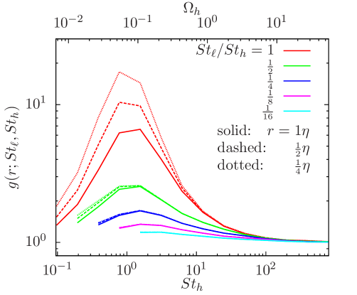
Figure 1.— The RDF as a function of the larger Stokes number, $St_{h}$, and the Stokes ratio, $f$. Lines of different colors show different values of $f$ in the range $\frac{1}{16}\leq f\leq 1$.

At a given $St_{h}$, the RDF decreases with decreasing Stokes ratio $f$. In general, the RDF between two different particles is smaller than the monodisperse RDF of each particle, i.e., $g(r,St_{\ell},St_{h})\leq g(r,St_{\ell},St_{\ell})$ and $g(r,St_{\ell},St_{h})\leq g(r,St_{h},St_{h})$ (Zhou et al. 2001). This is because particles of different sizes tend to cluster at different locations. If one continuously changes the particle size, the positions of maximum clustering intensity would shift spatially (see Pan et al. 2011). As the size difference of the two particles increases, the spatial separation between their local concentration peaks becomes larger, leading to a decreases in their “relative” clustering.

The RDF of different particles has also a much weaker $r$-dependence than for particles of the same size. As shown in Pan et al. (2011), the bidisperse RDF as a function of $r$ becomes flat and approaches a constant at small $r$ (see also Chun et al. 2005). Intuitively, the increases of the RDF toward small $r$ would eventually stop at scales below the typical separation between local concentration peaks of two different particle species. The flattering of the RDF toward small $r$ makes it easier to achieve convergence for particles of different sizes. At $f\leq 1/2$, the RDF already converges at $r\;\hbox to0.0pt{\lower 2.5pt\hbox{$\sim$}\hss}\raise 1.5pt\hbox{$>$}\;\eta/4$, except for the smallest two particles ($St_{\ell}=0.1$ and $St_{h}=0.19$) in our simulation.

To our knowledge, the effect of turbulent clustering on the collision kernel has not been included in existing dust coagulation models. As will be discussed in §3.4 and §5, neglecting this effect tends to underestimate the collision rate.

3.2. The Radial Relative Velocity

In Fig. 2, we show $\langle|w_{\rm r}|\rangle$ at fixed values of $f$. The red lines, corresponding to the monodisperse case, have been studied in Paper I (see Fig. 16 of Paper I), to which we refer the reader for details. The black lines plot the radial relative velocity, $\langle|w_{\rm f,r}|\rangle$, between the particle and the flow (or tracer) velocity at given distances, corresponding to $St_{\ell}=0$ or $f=0$. All the curves for $0<f<1$ lie in a region between the monodisperse and the particle-flow lines, which serve as useful delimiters.

Most theoretical models for the particle relative velocity predict its variance $\langle w^{2}\rangle$ (or $\langle w_{\rm r}^{2}\rangle$ for the radial component), which is easier to model than the mean relative velocity, $\langle|\boldsymbol{w}|\rangle$ (or $\langle|w_{\rm r}|\rangle$). The variance (or the rms) does not enter the collision kernel, but it is of theoretical importance, because understanding it helps reveal the underlying physics. The qualitative behavior of the mean radial relative velocity in Fig. 2 is very similar to the rms relative velocity shown in Figure 7 of Paper II for $\langle w^{2}\rangle^{1/2}$ (see also the right panel of Fig. 10 in Paper II for the radial rms $\langle w_{\rm r}^{2}\rangle^{1/2}$). Therefore, the successful physical explanation for the rms relative velocity in Paper II based on the Pan & Padoan model can also be used to understand the behavior of $\langle|w_{\rm r}|\rangle$ as a function of $St_{h}$ and $f$.

In the PP10 model, the relative velocity between two particles of any arbitrary sizes has two contributions, named the generalized shear and acceleration contributions. The generalized shear contribution represents the effect of the particles’ memory of the spatial flow velocity difference “seen” by the two particles at given times in the past. As the flow velocity difference, $\Delta u(\ell)$, scales with the length scale, $\ell$, the shear contribution depends on the separation, $d(t)$, of the two particles backward in time (i.e., at $t<0$). The memory timescale of an inertial particle is essentially its friction time, and the particles “forget” the flow velocity they saw before a friction time ago, i.e., at $t\;\hbox to0.0pt{\lower 2.5pt\hbox{$\sim$}\hss}\raise 1.5pt\hbox{$<$}\;-\tau_{\rm p}$. Thus, considering the particle separation (and hence $\Delta u(d(t))$) increases backward in time, the flow velocity difference, $\Delta u$, across the particle separation, $d(-\tau_{\rm p})$, at a friction time ago plays a crucial role in determining the shear contribution.

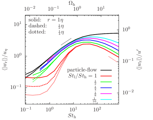
Figure 2.— Absolute average, $\langle|w_{\rm r}|\rangle$, of the radial relative speed normalized to $u_{\eta}$ (left Y-axis) and $u^{\prime}$ (right Y-axis). Black lines are the particle-flow relative velocity, corresponding to $f=0$. Dotted line segments denote $St_{h}^{1/2}$ (black) and $St_{h}^{-1/2}$ (red) scalings.

The generalized acceleration term reflects different responses of different particles to the flow velocity and is associated with the temporal flow velocity difference, $\Delta_{\rm T}u$, along individual particle trajectories (see Fig. 1 of Paper II for an illustration). The generalized acceleration contribution increases with the friction time difference, $\tau_{\rm p,h}-\tau_{\rm p,l}$. For particles of equal size, it vanishes, and only the generalized shear term contributes (Paper II). The generalized acceleration term is $r$-independent as it only depends on the temporal flow velocity statistics along individual particle trajectories (see Paper II for details). In Paper II, we showed that the prediction of the PP10 model for the rms relative velocity is in good agreement with the simulation results, confirming the physical picture of the model.

For particles of equal size, $\langle|w_{\rm r}|\rangle$ shows a strong $r-$ dependence at $St\;\hbox to0.0pt{\lower 2.5pt\hbox{$\sim$}\hss}\raise 1.5pt\hbox{$<$}\;1$. Due to the short memory/friction time, the particle distance $d(-\tau_{\rm p})$ a friction time ago is close to $r$, and thus $\Delta u(d(-\tau_{\rm p}))\simeq\Delta u(r)$, which is linear with $r$ for a small $r$. This gives rise to the $r$-dependence of the shear contribution. As $St$ increases, $d(-\tau_{\rm p})$ increases and becomes less sensitive to $r(=d(0))$. Thus, with increasing $St$, the relative velocity increases, and the $r-$dependence is weaker. At $St\;\hbox to0.0pt{\lower 2.5pt\hbox{$\sim$}\hss}\raise 1.5pt\hbox{$>$}\;6$, $\langle|w_{\rm r}|\rangle$ becomes $r-$ independent. Finally, for $\tau_{\rm p}\gg T_{\rm L}$, the flow velocity correlation/memory time is shorter than the particle memory, and the flow structures seen by the two particles within a friction time are incoherent. The action of the flow velocity on the particles is similar to random kicks in Brownian motion. This causes a reduction of the relative velocity by $(T_{\rm L}/\tau_{\rm p})^{1/2}$, leading to a $St^{-1/2}$ decrease in the $\tau_{\rm p}\gg T_{\rm L}$ limit. Intuitively, in this limit, the motions of larger particles are slower, and their relative velocity decreases with increasing $\tau_{\rm p}$.

At a given $St_{h}$, $\langle|w_{\rm r}|\rangle$ increases with decreasing $f$. This is due to the generalized acceleration contribution, which increases with increasing Stokes number difference. The PP10 model shows that the acceleration contribution dominates over the shear effect if the Stokes numbers differ by a factor of $\;\hbox to0.0pt{\lower 2.5pt\hbox{$\sim$}\hss}\raise 1.5pt\hbox{$>$}\;4$ (Paper II). In the case of $f=0$, $w_{\rm f,r}$ can be estimated by the temporal flow velocity difference, $\Delta u_{\rm T}(\Delta\tau)$, at a time lag of $\Delta\tau\simeq\tau_{\rm p}$ along the particle trajectory (see Paper II). Assuming that $\Delta u_{\rm T}$ can be approximated by Lagrangian temporal velocity difference $\Delta u_{\rm L}$, and that $\Delta u_{\rm L}\propto\Delta\tau^{1/2}$ for inertial-range time lags, this explains why $\langle|w_{\rm f,r}|\rangle$ increases approximately as $St^{1/2}$ (dotted line segment) for $\tau_{\rm p,h}$ in the inertial range. As $\Delta u_{\rm T}$ saturates at large time lags, $w_{\rm f,r}$ becomes constant for $\tau_{\rm p}\gg T_{\rm L}$. The $r-$dependence for particles of different sizes is much weaker than the case of equal-size particles, as the acceleration contribution is $r-$independent. At $f\leq 1/2$, $\langle|w_{\rm r}|\rangle$ already converges at $r=\frac{1}{4}\eta$. Together with the convergence of the RDF, this makes it easier to estimate the bidisperse collision kernel at $r\to 0$ than in the case of equal-size particles (see §3.3).

3.3. The Measured Collision Kernel

In Fig.  3, we plot the spherical collision kernel per unit cross section, $\Gamma^{\rm sph}/(\pi d^{2})=2g\langle|w_{\rm r}|\rangle$, normalized to $u_{\eta}$ and $u^{\prime}$ on the left and right Y-axes, respectively. The left panel shows the kernel for equal-size particles with $f=1$. The red lines in this panel is essentially the product of the red lines in Fig. 1 for $g$ and those in Fig. 2 for $\langle|w_{\rm r}|\rangle$. They correspond to the solid lines in Fig. 17 of Paper I. For convenience, we will also refer to the kernel per unit cross section as the normalized kernel.

For particles of equal size with $St\;\hbox to0.0pt{\lower 2.5pt\hbox{$\sim$}\hss}\raise 1.5pt\hbox{$>$}\;1$, the normalized kernel already converges at $r\;\hbox to0.0pt{\lower 2.5pt\hbox{$\sim$}\hss}\raise 1.5pt\hbox{$>$}\;\frac{1}{4}\eta$, as the $r-$dependences of $g$ and $\langle|w_{\rm r}|\rangle$ cancel out (see Paper I). However, for small particles with $St\;\hbox to0.0pt{\lower 2.5pt\hbox{$\sim$}\hss}\raise 1.5pt\hbox{$<$}\;1$, the kernel shows a significant $r-$dependence at $r\geq\frac{1}{4}\eta$. The decrease of $\langle|w_{\rm r}|\rangle$ with decreasing $r$ is faster than the increase of $g$, and the normalized kernel keeps decreasing in the $r$ range shown here. Since dust particle size in protoplanetary disks is much smaller than the Kolmogorov scale, the measured kernel for $St\;\hbox to0.0pt{\lower 2.5pt\hbox{$\sim$}\hss}\raise 1.5pt\hbox{$<$}\;1$ at $r\geq\frac{1}{4}\eta$ cannot be directly used in applications. One solution to this is to seek convergence of the normalized kernel by conducting larger simulations with a larger number of particles that allow accurate measurements at smaller scales. Alternatively, one may try to extrapolate the measured kernel to the $r\to 0$ limit using the physical picture and theoretical models for the problem. As the former is computationally expensive, we made an attempt in Paper I to pursue the latter approach.

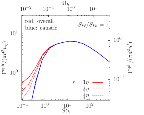
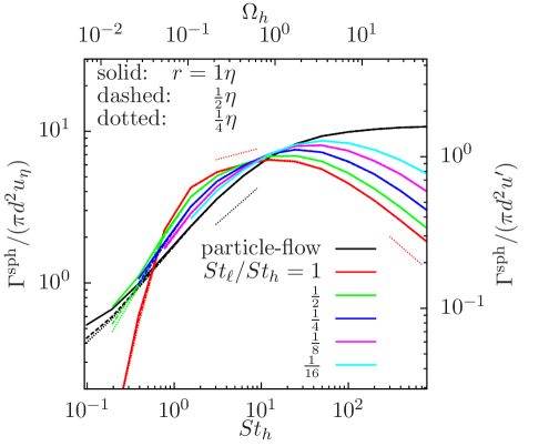
Figure 3.— Collision kernel per unit cross section in the spherical formulation. Left panel, the kernel for particles of equal sizes. The red lines show the overall kernel measured at different $f$. The blue lines are the $r$-independent contribution to the monodisperse kernel by caustic particle pairs with $w_{\rm r}\leq-0.2\,r/\tau_{\rm p}$. Right panel: the kernel for different Stokes ratios. Black lines plot the kernel between inertial and tracer particles ($f=0$). The red lines are the caustic contribution to the kernel for $f=1$, corresponding to the blue lines in the left panel. The red dotted line segments denote $St^{0.15}$ (left) and $St^{-1/2}$ (right) scalings, and the black one shows a $St^{1/2}$ scaling.

Theoretical models have shown that, at a given small distances, $r$, there are two types of particle pairs, whose contributions to the collision kernel have different scaling behaviors with $r$ (see Falkovich et al. 2002, Wilkinson et al. 2006). Following the terminology of Wilkinson et al. (2006), we named the two types of particle pairs “continuous” and “caustic” pairs in Paper I. As explained in details in Paper I, the two types correspond to the inner and outer parts of the probability distribution of $w_{\rm r}$ at small and large relative velocities, respectively.

Physically, the continuous particle pairs are located in flow regions with small velocity gradients, where the particles can efficiently respond to the flow. Their relative velocity for $St\;\hbox to0.0pt{\lower 2.5pt\hbox{$\sim$}\hss}\raise 1.5pt\hbox{$<$}\;1$ particles thus roughly follows the flow velocity difference across the particle distance. On the other hand, the caustic pairs correspond to flow regions with velocity gradients larger than $\simeq 1/\tau_{\rm p}$. In these regions, particle motions cannot catch up with the rapid flow velocity change, and their trajectories would deviate considerably from the flow elements. For example, particles may be shot out of the flow streamlines of high curvature (e.g., around a vortex), and these particles may cross the trajectories of nearby particles (Falkovich & Pumir 2007). At the trajectory crossing point, the particle velocity becomes multivalued, giving rise to the formation of folds, named caustics, in the momentum-position phase space (see, e.g., Fig. 1 of Gustavsson & Mehlig 2011). In contrast, the continuos pairs appear to be smooth in phase space. This difference in the phase space motivated the terminology for the two types of particle pairs (Wilkinson et al. 2006).

The relative velocity of continuous particle pairs decreases linearly with decreasing $r$, faster than the increase of the RDF. As a result, their contribution to the normalized kernel vanishes as $r\to 0$ (Gustavsson & Mehlig 2011, Hubbard 2012; see Fig. 19 in Paper I). On the other hand, the caustic contribution, corresponding to trajectory crossing events, is predicted to be $r-$independent, and it becomes dominant at $r\to 0$ (Gustavsson & Melig 2011). We thus attempted to isolate the $r-$independent caustic contribution.

Motivated by previous theoretical studies and our simulation data, we use a critical radial relative velocity, $w_{\rm c}$($<0$), to split approaching particle pairs into continuous ($w_{\rm c}\leq w_{\rm r}\leq 0$) and caustic ($w_{\rm r}\leq w_{\rm c}$) pairs. The contribution of caustic pairs to the kernel is then given by $\Gamma^{\rm cau}=-4\pi d^{2}g\int_{-\infty}^{w_{\rm c}}w_{\rm r}P(w_{\rm r})dw_{\rm r}$. Theoretical models suggest $w_{\rm c}\propto-r/\tau_{\rm p}$ (e.g., Falkovich et al. 2002; see PP10), but leave the coefficient in this estimate unfixed. There is thus a freedom for the choice of $w_{\rm c}$. As the caustic contribution is expected to be $r-$independent, we aim to select a value of $w_{\rm c}$ that minimizes the $r-$dependence of $\Gamma^{\rm cau}$. The best choice is found to be $w_{\rm c}=-0.2\,r/\tau_{\rm p}$. The blue lines in the left panel of Fig. 3 plot $\Gamma^{\rm cau}$ with this $w_{\rm c}$, and we see that the three lines for different $r$ almost all collapse onto a single curve. In Paper I, we set $w_{\rm c}=-r/\tau_{\rm p}$, with which $\Gamma^{\rm cau}$ still had a (weak) $r-$dependence (see Fig.  19 in Paper I). Setting $w_{\rm c}=-0.2\,r/\tau_{\rm p}$ appears to be a better choice for the purpose of obtaining an $r-$independent kernel contribution.

In the right panel of Fig. 3, the red lines are the caustic contribution for particles of equal sizes, corresponding to the blue lines in the left panel. All the other lines in the right panel show the normalized kernel for particles of different sizes. Unlike the case of equal-size particles, the kernels for particles of different sizes with $f\leq 1/2$ already converge at $r=\frac{1}{4}\eta$, and can thus be directly used in practical applications. As seen earlier, for $f\leq\frac{1}{2}$, both the RDF and $\langle|w_{\rm r}|\rangle$ converge at $r=\frac{1}{4}\eta$.

The black lines in the right panel plot the kernel between inertial particles and tracers, correspond to $f=0$. In this case, the RDF is unity, and the normalized kernel is simply calculated as $2\langle|w_{\rm f,r}|\rangle$ with $\langle|w_{\rm f,r}|\rangle$ the average of the radial component of the particle-flow relative velocity. The black lines and the red ones for $f=1$ provide useful limits, between which the curves for $0<f<1$ reside.

All curves of different $f$ appear to cross each other in a Stokes number range of $7\;\hbox to0.0pt{\lower 2.5pt\hbox{$\sim$}\hss}\raise 1.5pt\hbox{$<$}\;St_{h}\;\hbox to0.0pt{\lower 2.5pt\hbox{$\sim$}\hss}\raise 1.5pt\hbox{$<$}\;14$. In particular, at $St_{h}=12.4$, the variation of the normalized kernel is very small within $\;\hbox to0.0pt{\lower 2.5pt\hbox{$\sim$}\hss}\raise 1.5pt\hbox{$<$}\;10\%$ as $f$ changes from 0 to 1. We can thus assume that, for all values of $f$, the normalized kernels approximately cross at a common point around $St_{h}=12.4$ with $\Gamma^{\rm sph}/(\pi d^{2})\simeq u^{\prime}=6.8u_{\eta}$. This means that, if the larger particle has a friction time $\tau_{\rm p,h}\simeq T_{\rm L}=14.4\tau_{\eta}$, the kernel per unit cross section may be estimated by the 1D rms flow velocity, $u^{\prime}$, independent of the size of the smaller particle. The $f-$independence at $\tau_{\rm p,h}\simeq T_{\rm L}$ can be viewed as due to the cancelation of the dependences of the RDF and $\langle|w_{\rm r}|\rangle$ on $f$. At $St_{h}=12.4$, $\langle|w_{\rm r}|\rangle$ increases by a factor of 1.7 as $f$ goes from 1 to 0, while $g$ decreases by the same amount (Figs. 1 and 2).

Considering that the motions of particles with $\tau_{\rm p}\simeq T_{\rm L}$ are insensitive to turbulent eddies at small scales, the constancy of the kernel with $f$ at $\tau_{\rm p,h}\simeq T_{\rm L}$ is likely independent of the Reynolds number, $Re$, of the flow. However, as pointed out in §2, these particles couple to the driving scales of the turbulent flow, and their dynamics may be affected by how the flow is driven. Therefore, it remains to be confirmed whether the $f-$independence of the kernel at $\tau_{\rm p,h}\simeq T_{\rm L}$ is universal with respect to the flow driving mechanism. For such a confirmation, one needs to conduct a new set of simulations with different driving schemes, which are computationally expensive and beyond the scope of the current work.

For $\tau_{\rm p,h}\;\hbox to0.0pt{\lower 2.5pt\hbox{$\sim$}\hss}\raise 1.5pt\hbox{$>$}\;T_{\rm L}$, the kernel is larger at smaller $f$, because of the increase of $\langle|w_{\rm r}|\rangle$ with decreasing $f$. Interestingly, the opposite is seen for $1\;\hbox to0.0pt{\lower 2.5pt\hbox{$\sim$}\hss}\raise 1.5pt\hbox{$<$}\;St_{h}\;\hbox to0.0pt{\lower 2.5pt\hbox{$\sim$}\hss}\raise 1.5pt\hbox{$<$}\;12.4$, where the kernel is the smallest for $f=0$. As $f$ increases toward 1, the clustering effect is stronger, and the increase of the RDF more than compensates the decrease of $\langle|w_{\rm r}|\rangle$, lifting all the kernels for $f>0$ above the black lines. The particle-tracer kernel (black lines) simply follows the scaling of $\langle|w_{\rm f,r}|\rangle$ (since $g=1$), and goes like $St_{h}^{1/2}$ (dotted black line segment) in the inertial range. At $f>0$, the RDF increases as $St_{h}$ decrease toward 1, and the increase is more rapid at larger $f$ (see Fig. 1). Thus the slope of the normalized kernel with $St_{h}$ in the inertial range becomes continuously shallower as $f$ increases. For particles of equal sizes in the inertial range, the opposite trends of $g$ and $\langle|w_{\rm r}|\rangle$ with $St$ (red lines in Figs. 1 and 2) lead to a very flat slope: the normalized kernel scales with $St_{h}$ roughly as $St_{h}^{0.15}$ (the red dotted-line segment). For $0<f<1$, the slope of the kernel is in between 0.5 and 0.15. For example, the measured slope is approximately 0.22, 0.3, 0.35, 0.4, and 0.43 for $f=\frac{1}{2}$, $\frac{1}{4}$, $\frac{1}{8}$, $\frac{1}{16}$, and $\frac{1}{32}$, respectively. These features are not captured by the kernel formulation commonly used in dust coagulation models, as clustering effect is neglected.

In the right panel, we see that, for small particles with $St\;\hbox to0.0pt{\lower 2.5pt\hbox{$\sim$}\hss}\raise 1.5pt\hbox{$<$}\;1$, the kernels at different $f$ almost cross at another common point with $St_{h}=0.6$ and $\Gamma_{\rm sph}/(\pi d^{2})\simeq u_{\eta}$. Below $St_{h}=0.6$, the normalized kernel decreases as $f$ increases from 0 to 1, suggesting that, for small particles in the dissipation range, collisions of different particles are more frequent than between similar ones.

The collision kernel commonly used in dust coagulation models ignores the effect of clustering and adopts the model of Völk et al. (1980) and its successors for the particle relative velocity. At a given $St_{h}$, the Völk-type models predict larger relative velocity between particles of different sizes than between particles of equal size (see, e.g., Ormel & Cuzzi 2007). Therefore, the commonly-used kernel is smallest at $f=1$ and the largest at $f=0$ for any $St_{h}$. This trend is consistent with our results for $St_{\rm h}\;\hbox to0.0pt{\lower 2.5pt\hbox{$\sim$}\hss}\raise 1.5pt\hbox{$<$}\;1$ and $\tau_{\rm p,h}\;\hbox to0.0pt{\lower 2.5pt\hbox{$\sim$}\hss}\raise 1.5pt\hbox{$>$}\;T_{\rm L}$, but is incorrect for $\tau_{\rm p,h}$ in the inertial range, where the clustering effect makes the kernel largest at $f=1$. Equation (28) of Ormel & Cuzzi (2007) for the rms relative velocity of inertial-range particles suggests that, in the commonly-used prescription, the normalized collision kernel for $f=0$ is larger by a factor of 1.5 than for $f=1$. On the other hand, our simulation data indicates that, in the inertial range, the kernel for $f=1$ is larger than the $f=0$ case by a factor of a few. As discussed in §3.5, in a realistic disk turbulence with a much larger Reynolds number than our simulated flow, the collision kernel for inertial-range particles of equal size ($f=1$) may exceed the kernel at $f\to 0$ by a significantly larger amount, if the RDF, $g$, has a significant Reynolds number dependence.

We also computed the cylindrical kernel $\Gamma^{\rm cyl}$ and found it almost coincides with $\Gamma^{\rm sph}$ except for small particles of similar sizes with $St_{h}\ll 1$ (see §3.4). As mentioned earlier, the two formulations give equal estimate for the kernel if the direction of ${\boldsymbol{w}}$ is isotropic. In the cylindrical formulation, we can also split particle pairs of equal size into two types using a critical value, $|{\boldsymbol{w}}|_{\rm c}$, for the 3D relative velocity amplitude, $|{\boldsymbol{w}}|$. Particle pairs with $|{\boldsymbol{w}}|\geq|{\boldsymbol{w}}|_{\rm c}$ and $|{\boldsymbol{w}}|<|{\boldsymbol{w}}|_{\rm c}$ are counted as continuous and caustic pairs, respectively. With the choice of $|{\boldsymbol{w}}|_{\rm c}=0.27r/\tau_{\rm p}$, the caustic contribution to the cylindrical kernel per unit cross section, $g\int_{|{\boldsymbol{w}}|_{\rm c}}^{\infty}|{\boldsymbol{w}}|P(|{\boldsymbol{w}}|)d|{\boldsymbol{w}}|$, is $r-$independent and is almost equal to the caustic contribution from the spherical formulation. Note that the critical value $|{\boldsymbol{w}}|_{\rm c}=0.27r/\tau_{\rm p}$ is different from the one used in the spherical formulation, and it is also different from the choice of $|{\boldsymbol{w}}|_{\rm c}=r/\tau_{\rm p}$ by Hubbard (2013).

We point out that there are uncertainties in the way to split the continuous and caustic pairs for small particles of equal size ($St\;\hbox to0.0pt{\lower 2.5pt\hbox{$\sim$}\hss}\raise 1.5pt\hbox{$<$}\;1$, $f=1$). Theoretical models suggest that the critical relative velocity $w_{\rm c}$ (or $|{\boldsymbol{w}}|_{\rm c}$) scales as $\propto r/\tau_{\rm p}$, but do not predict its exact value. We selected a value $w_{\rm c}$ to obtain an $r-$independent contribution to the kernel, but there is no theoretical guarantee of the accuracy of our choice for $w_{\rm c}$. It is possible that the $r-$independent caustic contribution we obtained at $r\;\hbox to0.0pt{\lower 2.5pt\hbox{$\sim$}\hss}\raise 1.5pt\hbox{$>$}\;\frac{1}{4}\eta$ may not precisely represent the realistic kernel as $r\to 0$. In other words, as $r$ decreases below $\frac{1}{4}\eta$, the critical relative velocity $w_{\rm c}$ that minimizes the $r-$dependence could be different from the value we selected. Another uncertainty is that it is not clear whether, at the distance range we measured, the two types of pairs can be precisely divided simply by a single critical value for the relative velocity. The transition from continuous to caustic types may not occur sharply at a single relative velocity. Instead, the transition could be gradual, occurring over a relative velocity range, where particle pairs may not be definitely counted as continuous or caustic. Due to these uncertainties, the caustic kernel we obtained should be tested by future simulations that can measure the kernel at smaller scales, where the caustic contribution dominates.

Despite the uncertainties, we think that the method of splitting two types of pairs is useful to provide physical insights to understanding the $r-$dependence of the collision kernel at $St\;\hbox to0.0pt{\lower 2.5pt\hbox{$\sim$}\hss}\raise 1.5pt\hbox{$<$}\;1$ and $f=1$ in the $r-$range explored. We also found that it gives a reasonable estimate for small equal-size particles at $r\to 0$. Wilkinson et al. (2006) predict that, for these particles, the normalized kernel at $r\to 0$ is given by $\propto\exp(-A/St)$, similar to an activation process. Our measured caustic kernel is in good agreement with this prediction using an activation threshold of $A\simeq 1.0$.

Hubbard (2012) argued that, in the monodisperse case, inertial particles that show significant clustering do not contribute to the collision rate, i.e., the particles that cluster are non-collisional. In our terminology, this argument essentially assumes that clustering is mainly caused by the continuous particle pairs, which do not contribute to the collision rate at $r\to 0$, while the caustic pairs that contribute to the collision rate do not significantly contribute to clustering. This is likely true for particles of equal size with $St\;\hbox to0.0pt{\lower 2.5pt\hbox{$\sim$}\hss}\raise 1.5pt\hbox{$<$}\;1$. For these small particles, caustic pairs are very rare and make only a tiny fraction of the total number of particle pairs at a given small distance. Thus, the main contribution to clustering must be due to the rest of the particles, i.e., particle pairs of the continuous type. As discussed earlier, the continuous pairs do not contribute to the collision kernel, as the particle distance (or size), $r$, approaches zero (Wilkinson et al. 2006, Hubbard 2012).

However, our data indicates that the argument of Hubbard (2012) is invalid for inertial-range particles with $\tau_{\eta}\;\hbox to0.0pt{\lower 2.5pt\hbox{$\sim$}\hss}\raise 1.5pt\hbox{$<$}\;\tau_{\rm p}\;\hbox to0.0pt{\lower 2.5pt\hbox{$\sim$}\hss}\raise 1.5pt\hbox{$<$}\;T_{\rm L}$. In Paper I, we showed that caustic pairs start to dominate at $St\;\hbox to0.0pt{\lower 2.5pt\hbox{$\sim$}\hss}\raise 1.5pt\hbox{$>$}\;1$, and, at $St\;\hbox to0.0pt{\lower 2.5pt\hbox{$\sim$}\hss}\raise 1.5pt\hbox{$>$}\;3.11$, most particle pairs belong to the caustic type. Therefore, if significant clustering occurs for inertial-range particles, it must be from caustic pairs. Fig. 1 shows that the RDF, $g$, is significantly above unity for inertial-range particles of equal size, suggesting that caustic particles do contribute to clustering. In fact, it is the clustering of the caustic pairs that makes the normalized kernel for particles of equal size in the inertial range larger than that between particles of different sizes. Thus, for inertial-range particle of equal size, it is not true that the clustering particles do not collide.

For particle of different sizes, the RDF, the relative velocity and hence the kernel all converge at $r\;\hbox to0.0pt{\lower 2.5pt\hbox{$\sim$}\hss}\raise 1.5pt\hbox{$>$}\;\frac{1}{4}\eta$, and it is thus not necessary to split the pairs into the two types. In Fig. 1, we see that, for a Stokes ratio of $f\;\hbox to0.0pt{\lower 2.5pt\hbox{$\sim$}\hss}\raise 1.5pt\hbox{$>$}\;\frac{1}{4}$, there is a moderate degree of clustering at $St_{h}\simeq 1$. Since the kernel for $f\;\hbox to0.0pt{\lower 2.5pt\hbox{$\sim$}\hss}\raise 1.5pt\hbox{$>$}\;\frac{1}{4}$ and $St_{h}\simeq 1$ already converges at $r=\frac{1}{4}\eta$, all particle pairs at that distance contribute to the collision rate. Therefore, clustering at $f\;\hbox to0.0pt{\lower 2.5pt\hbox{$\sim$}\hss}\raise 1.5pt\hbox{$>$}\;\frac{1}{4}$ and $St_{h}\simeq 1$ would contribute to increase the collision rate, again in contrast to the argument of Hubbard (2012). In summary, the claim of Hubbard (2012, 2013) that the clustering particles do not contribute to the collision rate is not valid in general and applies only for the special case of small equal-size particles with $St\;\hbox to0.0pt{\lower 2.5pt\hbox{$\sim$}\hss}\raise 1.5pt\hbox{$<$}\;1$.

3.4. Comparing with Commonly-used Kernel Formula

The kernel formula commonly used in dust coagulation models is $\Gamma^{\rm com}=\pi d^{2}\langle w^{2}\rangle^{1/2}$, where the rms relative velocity, $\langle w^{2}\rangle^{1/2}$, is usually taken from the model of Völk et al. (1980) or its successors. $\Gamma^{\rm com}$ is in a simpler form than $\Gamma^{\rm sph,cyl}$, and in this section we use our simulation data to assess the accuracy of the simplified formula for the collision kernel. We defer a systematic test of Völk-type models for $\langle w^{2}\rangle^{1/2}$ to a later work.

In comparison to the spherical and cylindrical kernels $\Gamma^{\rm sph,cyl}$, $\Gamma^{\rm com}$ neglects the clustering effect, and uses the 3D rms of the relative velocity rather than the mean relative velocity, $\langle|w_{\rm r}|\rangle$ or $\langle|{\boldsymbol{w}}|\rangle$. The ratios of $\Gamma^{\rm sph,cyl}$ to $\Gamma^{\rm com}$ can be written as $gC_{12}^{\rm sph,cyl}$, where $C_{12}^{\rm sph}\equiv 2\langle|w_{\rm r}|\rangle/\langle w^{2}\rangle^{1/2}$ and $C_{12}^{\rm cyl}\equiv\langle|{\boldsymbol{w}}|\rangle/\langle w^{2}\rangle^{1/2}$. The ratios $C_{12}^{\rm sph,cyl}$ compare the mean and rms relative speeds, corresponding to the first- and second- order moments of ${\boldsymbol{w}}$, respectively. In the left panel Fig. 4, we show $C_{12}^{\rm sph}$ (solid) and $C_{12}^{\rm cyl}$ (dashed) computed from our simulation data at $r=\eta/4$. For all Stokes pairs, the ratios are smaller than unity, meaning that using the rms relative velocity tends to overestimate the kernel. Except for a small difference of $5\%$ at $St_{h}\ll 1$ and $f=1$, the solid lines almost coincide with the dashed ones, suggesting that $2\langle|w_{\rm r}\rangle=\langle|{\boldsymbol{w}}|\rangle$, and hence $\Gamma^{\rm sph}=\Gamma^{\rm cyl}$, within an uncertainty of only 5%. The near equality of $\Gamma^{\rm sph}\simeq\Gamma^{\rm cyl}$ was expected under the assumption of isotropy for the direction of ${\boldsymbol{w}}$.

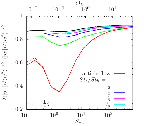
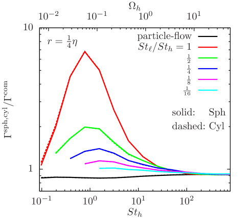
Figure 4.— Left panel: the mean to rms ratios, $C_{12}^{\rm sph}\equiv 2\langle|w_{\rm r}|\rangle/\langle w^{2}\rangle^{1/2}$ (solid) and $C_{12}^{\rm cyl}\equiv\langle|{\boldsymbol{w}}|\rangle/\langle w^{2}\rangle^{1/2}$ (dashed), at $r=\frac{1}{4}\eta$. Right panel: The ratios of spherical (solid) and cylindrical (dashed) kernels to the commonly-used formulation, $\Gamma^{\rm com}=\pi d^{2}\langle w^{2}\rangle^{1/2}$. The effect of turbulent clustering is not accounted for in the commonly-used kernel, $\Gamma^{\rm com}$. The kernels are measured at $r=\frac{1}{4}\eta$.

The ratios, $C_{12}^{\rm sph,cyl}$, depend on the shape of the probability distribution function of ${\boldsymbol{w}}$, particularly on the central part of the PDF, as both the mean and the rms are low-order moments. If ${\boldsymbol{w}}$ is Gaussian, the PDF of the 3D amplitude $|{\boldsymbol{w}}|$ is Maxwellian, and it is easy to show $C_{12}^{\rm cyl}=({8/3\pi})^{1/2}\simeq 0.92$. The same value is expected for $C_{12}^{\rm sph}$. As the radial rms relative speed, $\langle w_{\rm r}^{2}\rangle^{1/2}$, is typically smaller than the 3D rms, $\langle w^{2}\rangle^{1/2}$, by a factor of $\sqrt{3}$ (see Paper II), we have $C_{12}^{\rm sph}\simeq(4/3)^{1/2}\langle|w_{\rm r}|\rangle/\langle w_{\rm r}^{2}\rangle^{1/2}$. With a Gaussian distribution for $w_{\rm r}$, $\langle|w_{\rm r}|\rangle/\langle w_{\rm r}^{2}\rangle^{1/2}=({2/\pi})^{1/2}$, and thus $C_{12}^{\rm sph}$ is also equal to $(8/3\pi)^{1/2}$. A value of $\simeq 0.92$ for $C_{12}^{\rm sph,cyl}$ is observed in the left panel of Fig. 4 at $\tau_{\rm p,h}\gg T_{\rm L}$, where the PDF of ${\boldsymbol{w}}$ is approximately Gaussian (see Paper III).

As discussed in Paper I, the mean to rms ratios are smaller if the PDF of ${\boldsymbol{w}}$ is non-Gaussian with a sharper inner part and fatter tails (see Fig.  16 of Paper I). For particles of equal size with $\tau_{\rm p}\;\hbox to0.0pt{\lower 2.5pt\hbox{$\sim$}\hss}\raise 1.5pt\hbox{$<$}\;T_{\rm L}$, the PDF is highly non-Gaussian with very fat tails, and the ratios $C_{12}^{\rm sph,cyl}$ are significantly smaller than 0.92. In particular, the degree of non-Gaussianity peaks at $St\simeq 1$, leading to a dip in the ratio at $St\simeq 1$, where $C_{12}^{\rm sph,cyl}\simeq 0.3-0.4$. In Paper III, we showed that the non-Gaussianity of the relative velocity PDF decreases with decreasing Stokes ratio $f$, and this is responsible for the increase of $C_{12}^{\rm sph,cyl}$ as $f$ decreases toward 0. In the case of $f=0$, the inner part of the PDF for the particle-flow relative velocity is nearly Gaussian for all particles (see Fig. 1 of Paper III), which explains why the black lines for $f=0$ are close to 0.9 at all $St$. The left panel of Fig. 4 suggests that using the rms instead of the mean relative velocity in the collision kernel tends to overestimate the collision rate, especially for particles of similar sizes.

We also computed $C_{12}^{\rm sph,cyl}$ at other distances, $r$. For $f\;\hbox to0.0pt{\lower 2.5pt\hbox{$\sim$}\hss}\raise 1.5pt\hbox{$<$}\;\frac{1}{2}$, the ratio converges at $r=\frac{1}{4}\eta$, corresponding to the convergence of the PDF shape found in §4.2 of Paper III. But for particles of equal size with $St\;\hbox to0.0pt{\lower 2.5pt\hbox{$\sim$}\hss}\raise 1.5pt\hbox{$<$}\;6$, $C_{12}^{\rm sph,cyl}$ have not converged and decrease with decreasing $r$ due to the fatter PDF shape at smaller $r$ (Paper I). For these particles, the ratios at $r\;\hbox to0.0pt{\lower 2.5pt\hbox{$\sim$}\hss}\raise 1.5pt\hbox{$<$}\;\eta/4$ could be significantly smaller than the values shown in the left panel of Fig. 4.

In Fig. 4, we plot the ratio, $\Gamma^{\rm sph,cyl}/\Gamma^{\rm com}$, in our simulation. In the calculation of $\Gamma^{\rm com}$, we used the 3D rms relative velocity measured from our data. Again, the near coincidence of the solid and dashed lines for $\Gamma^{\rm sph}$ and $\Gamma^{\rm cyl}$ indicates that the two formulations give similar estimates for the collision rate. In the limit $f\to 0$ (black lines), the ratio of the commonly-used formula to $\Gamma^{\rm sph,cyl}$ is about 0.9 at all $St_{h}$, meaning that it overestimates the kernel slightly by $\;\hbox to0.0pt{\lower 2.5pt\hbox{$\sim$}\hss}\raise 1.5pt\hbox{$<$}\;10\%$. For this particle-tracer case, the RDF $g$ is unity, and the overestimate is because $\langle w^{2}\rangle^{1/2}$ is larger than $2\langle|w_{\rm r}\rangle$ by 10% (see the left panel). For $f\;\hbox to0.0pt{\lower 2.5pt\hbox{$\sim$}\hss}\raise 1.5pt\hbox{$<$}\;\frac{1}{4}$, $\Gamma^{\rm com}$ is a good approximation to the collision kernel except for an overestimate of $\;\hbox to0.0pt{\lower 2.5pt\hbox{$\sim$}\hss}\raise 1.5pt\hbox{$<$}\;40\%$ at $St_{h}\simeq 1$.

For particles of similar sizes ($f=1$ and $\frac{1}{2}$), the ratios of $\Gamma^{\rm sph,cyl}$ to $\Gamma^{\rm com}$ are close to unity for $\tau_{\rm p}\;\hbox to0.0pt{\lower 2.5pt\hbox{$\sim$}\hss}\raise 1.5pt\hbox{$>$}\;T_{\rm L}$, but become significantly larger as $St_{h}$ decreases in the inertial range toward $\simeq 1$. This means that $\Gamma^{\rm com}$ underestimates the kernel for particles of similar sizes in the inertial range and in particular at $St_{h}\simeq 1$. The ratios $\Gamma^{\rm sph,cyl}/\Gamma^{\rm com}$ converge at $r=\frac{1}{4}\eta$ except for $f=1$. For equal-size particles, $\Gamma^{\rm sph,cyl}/\Gamma^{\rm com}$ keeps increasing as $r$ decreases to $\frac{1}{4}\eta$, and the underestimate of $\Gamma^{\rm com}$ would be more severe at $r<\frac{1}{4}\eta$. In general, how $\Gamma^{\rm com}$ compares to $\Gamma^{\rm sph,cyl}$ depends on two opposite effects: using the rms relative velocity instead of the mean tends to overestimate the collision rate, while neglecting the clustering effect causes an underestimate. Both effects are strongest for particles of similar sizes at $St_{h}\simeq 1$ (see the left panel of Fig. 4 and Fig. 1), but it turns out that the second effect dominates for $St_{h}$ in the inertial range, where $g$ is significantly larger than $1/C_{12}^{\rm sph,cyl}$. Another interesting consequence of neglecting clustering is that, as $f$ decreases from 1 to 0, $\Gamma^{\rm com}$ increases because $\langle w^{2}\rangle$ is larger at smaller $f$ (see Fig. 7 of paper II). This is in contrast to the result shown in the right panel of Fig. 3, where the kernel decreases with decreasing $f$ for $St_{h}$ in the inertial range.

In summary, the commonly-used kernel formula provide a good approximation for very different particles with the Stoke ratio $f\;\hbox to0.0pt{\lower 2.5pt\hbox{$\sim$}\hss}\raise 1.5pt\hbox{$<$}\;\frac{1}{4}$ or if the larger particle has $\tau_{\rm p,h}\;\hbox to0.0pt{\lower 2.5pt\hbox{$\sim$}\hss}\raise 1.5pt\hbox{$>$}\;T_{\rm L}$. However, it significantly underestimates the collision rate for particles of similar sizes (with $f\;\hbox to0.0pt{\lower 2.5pt\hbox{$\sim$}\hss}\raise 1.5pt\hbox{$>$}\;\frac{1}{2}$) with $\tau_{\rm p,h}\;\hbox to0.0pt{\lower 2.5pt\hbox{$\sim$}\hss}\raise 1.5pt\hbox{$<$}\;T_{\rm L}$, especially for $St_{\rm h}\simeq 1$.

3.5. Extrapolation to Realistic Reynolds Numbers

Due to the limited numerical resolution, the Reynolds number, $Re$, of our simulated flow is only $\simeq 10^{3}$, much smaller than the typical value of $Re\simeq 10^{6}-10^{8}$ in protoplanetary disks. To study dust particles in protoplanetary turbulence, the results of our simulation should be appropriately extrapolated to a realistic $Re$. An accurate extrapolation requires the $Re-$dependence of the collision kernel, which is currently unknown. Here we offer some speculations on how to extrapolate the measured results to higher $Re$. Studies of the $Re-$dependence using higher-resolution simulations will be conducted in future work.

In our simulation, the inertial range is short, and the timescale separation between the driving scale and the Kolmogorov scale is only one order of magnitude. More precisely, we have $T_{\rm L}/\tau_{\eta}\simeq 14.4$ in our flow. Although we count all particles with $\tau_{\eta}\;\hbox to0.0pt{\lower 2.5pt\hbox{$\sim$}\hss}\raise 1.5pt\hbox{$<$}\;\tau_{\rm p}\;\hbox to0.0pt{\lower 2.5pt\hbox{$\sim$}\hss}\raise 1.5pt\hbox{$<$}\;T_{\rm L}$ inertial-range particles, strictly speaking, there is only one species of particles in our simulation that are definitely not affected by either the dissipation or the driving scales of the flow (Paper III). This species is particles with $\tau_{\rm p}=6.21\tau_{\eta}$, or equivalently $\tau_{\rm p}=0.43T_{\rm L}$. Particles with $\tau_{\rm p}\;\hbox to0.0pt{\lower 2.5pt\hbox{$\sim$}\hss}\raise 1.5pt\hbox{$>$}\;0.43T_{\rm L}$ are coupled to eddies significantly above the dissipation range, and their dynamics is insensitive to the smallest eddies in the flow. Thus, when normalized to the flow properties at driving scales, the collision statistics of these particles is expected to be independent of $Re$. Our measured kernel for these particles can be directly applied to corresponding particles with $\Omega\equiv\tau_{\rm p}/T_{\rm L}\;\hbox to0.0pt{\lower 2.5pt\hbox{$\sim$}\hss}\raise 1.5pt\hbox{$>$}\;0.43$ in protoplanetary disks. Therefore, we only need extrapolations for $\Omega\;\hbox to0.0pt{\lower 2.5pt\hbox{$\sim$}\hss}\raise 1.5pt\hbox{$<$}\;0.43$ particles in the inertial and dissipation ranges of the real flow.

As $Re$ increases, the separation between $\tau_{\eta}$ and $T_{\rm L}$ increases as $Re^{1/2}$. Considering that $Re\simeq 10^{3}$ and $T_{\rm L}/\tau_{\eta}\simeq 14.4$ in our flow, we have $\Omega\simeq 2.2Re^{-1/2}St$ for larger $Re$. This suggests that, if the driving of the flow is fixed, then, with increasing $Re$, $St=1$ particles correspond to smaller size with $\Omega\simeq 2.2Re^{-1/2}$. Particles with $2.2Re^{-1/2}\;\hbox to0.0pt{\lower 2.5pt\hbox{$\sim$}\hss}\raise 1.5pt\hbox{$<$}\;\Omega\;\hbox to0.0pt{\lower 2.5pt\hbox{$\sim$}\hss}\raise 1.5pt\hbox{$<$}\;1$ lie in the inertial range, and we need to extrapolate the kernel down to $\Omega\simeq 2.2Re^{-1/2}$.

A simple extrapolation is to assume that the measured slope for the normalized kernel in the inertial range (see Fig. 3) is independent of the Reynolds number. With this assumption, the normalized kernel for equal-size particles ($f=1$) in the inertial range is approximately given by $\simeq u^{\prime}\Omega^{0.15}$, while in the $f\to 0$ limit it scales as $\simeq u^{\prime}\Omega^{1/2}$ (see Fig. 3 and §3.3). In this case, the effect of clustering significantly enhances the kernel for all inertial-range particles of similar sizes. Interestingly, with this extrapolation, we find that, for a realistic value of $Re\;\hbox to0.0pt{\lower 2.5pt\hbox{$\sim$}\hss}\raise 1.5pt\hbox{$>$}\;10^{6}-10^{8}$, the normalized kernel for equal-size particles at $St_{h}=1$ (corresponding to $\Omega_{\rm h}=2.2\times 10^{-3}-2.2\times 10^{-4}$) is larger by a factor of 10-20 than the particle-tracer limit with $f\to 0$. This suggests significantly higher collision frequency between similar particles than between particles of different sizes, as the particles just grow into the inertial range. Note that, in our flow with low $Re$, the variation of the kernel at $St_{\rm h}=1$ is quite small, increasing only by a factor of $\leq 2$ as $f$ increases from $0$ to $1$ (see Fig. 3).

In the extrapolation above for equal-size particles, an implicit assumption was made for the scaling of the RDF with $\Omega$ in the inertial range. Since the relative velocity is expected to scale as $\propto\Omega^{1/2}$ (or $St^{1/2}$) in the inertial range, the assumed $\Omega^{0.15}$ scaling for the normalized kernel, $\Gamma^{\rm sph}/\pi d^{2}$ ($\equiv 2g\langle|w_{\rm r}|\rangle$), holds only if the RDF increases with decreasing $\Omega$ as $\propto\Omega^{-0.35}$ in the inertial range. The RDF for $f=1$ in our flow does not have a clear power-law range with $\Omega$ (see Fig. 1). As mentioned earlier, strictly only one species of particles ($St=6.21$) lie in the inertial range in our flow, and it is possible that $g$ may show an extended power-law scaling with $\Omega$ in a high$-Re$ flow with a wider range of scales unaffected by the dissipation or the driving scales. The possibility, however, needs to be verified by simulations at higher resolutions.

If the scaling $g\propto\Omega^{-0.35}$ is valid for particles in the inertial range, it would imply a $Re-$dependence of the RDF for particles at fixed Stokes numbers, $St$. Inserting $\Omega\propto Re^{-1/2}St$ to this scaling gives $g(St\simeq 1)\propto Re^{0.175}$ for $St\simeq 1$ particles in turbulent flows of different $Re$. The $Re-$dependence of the RDF at fixed Stokes numbers around or below unity have been studied in the literature, but, to our knowledge, a conclusive answer is still lacking. For example, the simulation of Collins & Keswani (2004) indicated that the RDF of $St\simeq 1$ particles converges already at $Re\simeq 600$ (see also Hogan & Cuzzi 2001), while Falkovich & Pumir (2004) found that the clustering intensity shows a significant increase with increasing $Re$.

Clearly, if the $Re$-dependence of the RDF at $St\simeq 1$ is weaker than $Re^{0.175}$, the increase of $g$ with decreasing $\Omega$ would be slower than $\Omega^{-0.35}$, and thus the scaling of the normalized kernel for $f=1$ would be steeper than $\Omega^{0.15}$. An extreme case is that the RDF for $St$ fixed around $\simeq 1$ is independent of $Re$. In that case, the RDF for inertial-range particles with $\tau_{\rm p}$ significantly away from the dissipation scales can only vary slowly with $\Omega$, and, for these particles, the normalized kernel would scale as $\Omega^{1/2}$, as it just follows scaling of the relative velocity. This scaling is similar to the $f\to 0$ limit. Therefore, we would expect the kernels for $f=1$ and $f\to 0$ to remain close to each other as $\Omega_{h}$ decreases in the inertial range. In the inertial range, clustering does not considerably increase the collision rate of similar-size particles. Only as $St_{h}$ approaches 1, would the monodisperse RDF start to increase significantly, which would tend to increase the kernel for $f=1$ above the $f\to 0$ case by a factor of 2 or so. This behavior is in contrast to the extrapolation based on the slope of the normalized kernel measured in our simulation.

In summary, the extrapolation of the measured kernel from our simulation to a realistic flow with much larger $Re$ is uncertain. If we assume that the measured slope of the normalized kernel at fixed $f$ can be applied to larger $Re$, then the decrease of the kernel for $f=1$ with decreasing $\Omega$ in the inertial range is slower than the limit $f\to 0$, and, at $\tau_{\rm p,h}\simeq\tau_{\eta}$, the collision rate between similar particles is much larger than between different particles. On the other hand, if the RDF at a fixed Stokes number $St$ around unity is $Re-$independent, then the normalized kernels for $f=1$ and $f=0$ have a similar scaling with $\Omega_{h}$ and likely stay close to each other for any $\Omega_{h}$ in the inertial range. This question will be settled with future higher-resolution ($\geq 1024^{3}$) simulations, where the scalings of $g$ and of the normalized kernel with $\Omega$ (in the inertial range), and the $Re-$dependence of $g$ at fixed Stokes numbers can be checked.

4. The Collision-Rate Weighted Statistics

Coagulation models for dust particle growth need not only the collision kernel to calculate the collision rate, but also the collision velocity or collision energy to determine the collision outcome. While a small collision velocity favors particle sticking and growth, a large impact velocity leads to bouncing or destruction of the colliding particles. Until recently, dust coagulation models usually adopted a single collision velocity, typically the rms, to judge the collision outcome of two particles of given sizes. However, due to the stochastic nature of turbulence, the collision velocity for each size pair is not single-valued, but has a probability distribution. Thus, even for particles of exactly the same properties, the collision outcome can be different, and the probability distribution function (PDF) of the collision velocity is needed to calculate the fractions of collisions resulting in sticking, bouncing and fragmentation. Windmark et al. (2012) and Garaud et al. (2013) have shown that accounting for the collision velocity PDF makes a significant difference in the predicted particle size evolution in protoplanetary disks.

Garaud et al. (2013) emphasized that the collision velocity PDF to be used in a coagulation model should include a collision-rate weighting factor to account for the higher collision frequency of particle pairs with larger relative velocity. The importance of collision-rate weighting was also pointed out by Hubbard (2012), who argued that the commonly-used rms relative velocity with equal weight for each nearby particle pair is not appropriate for applications to dust particle collisions. A collision-rate weighted rms was proposed by Hubbard (2012). In Papers II and III, we have systematically studied the unweighted rms and PDF of turbulence-induced relative velocity. In this section, we compute the collision-rate weighted statistics from our simulation data.

In the cylindrical kernel formulation, the collision rate is $\propto|{\boldsymbol{w}}|$, and the collision-rate weighted distribution of the 3D amplitude can be obtained from the unweighted PDF, $P(|\boldsymbol{w}|)$, simply by $P_{\rm cyl}(|\boldsymbol{w}|)=|\boldsymbol{w}|P(|\boldsymbol{w}|)/\langle|\boldsymbol{w}|\rangle$ (see eq. (36) in Garaud et al. 2013). The weighted PDF of $|\boldsymbol{w}|$ in the spherical formulation is more complicated, and in terms of the PDF, $P_{\rm v}(\boldsymbol{w})$ of the vector ${\boldsymbol{w}}$, it can be defined as,

$$P_{\rm sph}(|\boldsymbol{w}|)=-\frac{1}{N}\int\limits_{\pi/2}^{\pi}d\theta\int\limits_{0}^{2\pi}d\phi\sin(\theta)\cos(\theta)|{\boldsymbol{w}}|^{3}P_{\rm v}(|\boldsymbol{w}|,\theta,\phi),$$ (2)

where a weighting factor $-w_{\rm r}$($=|{\boldsymbol{w}}|\cos(\theta)$) is applied and the integration limits for $\theta$ count only approaching pairs with negative $w_{\rm r}$. The normalization factor is $N=-\int_{-\infty}^{0}w_{\rm r}P(w_{\rm r})dw_{\rm r}$, with $P(w_{\rm r})$ the PDF of the radial component.

If the direction of ${\boldsymbol{w}}$ is isotropic relative to ${\boldsymbol{r}}$, we have $P_{\rm v}(|{\boldsymbol{w}}|,\theta,\phi)=P_{\rm v}(|{\boldsymbol{w}}|)$, and a calculation of the double integral in eq. (2) gives $-\pi|{\boldsymbol{w}}|^{3}P_{\rm v}(|\boldsymbol{w}|)$. Using eq. (1) for $P(w_{\rm r})$, it is easy to show that $N=\pi\int_{0}^{\infty}|{\boldsymbol{w}}|^{3}P_{\rm v}(|{\boldsymbol{w}}|)d|{\boldsymbol{w}}|$. We thus have $P_{\rm sph}(|\boldsymbol{w}|)=|{\boldsymbol{w}}|^{3}P_{\rm v}(|\boldsymbol{w}|)/\int_{0}^{\infty}|{\boldsymbol{w}}|^{3}P_{\rm v}(|{\boldsymbol{w}}|)d|{\boldsymbol{w}}|$, which is identical to $P_{\rm cyl}(|\boldsymbol{w}|)$. Therefore, the weighted PDFs of the 3D amplitude, $|{\boldsymbol{w}}|$, with the spherical and cylindrical formulations are equal under the isotropy assumption for ${\boldsymbol{w}}$.

We measure $P_{\rm sph}(|\boldsymbol{w}|)$ from our simulation data as $P_{\rm sph}(|\boldsymbol{w}|)=\sum_{i}H(-w_{\rm r}^{(i)})w_{\rm r}^{(i)}\delta(|\boldsymbol{w}|-|\boldsymbol{w}|^{(i)})/\sum_{i}H(-w_{\rm r}^{(i)})w_{\rm r}^{(i)}$, where the sum is over all particle pairs available at a given small distance and $H$ is the Heaviside step function to exclude the separating particle pairs moving away from each other. The PDF measured this way is consistent with $P_{\rm sph}(|\boldsymbol{w}|)$ defined by eq. (2).

4.1. The Collision-Rate Weighted RMS

We start by considering the collision-rate weighted rms relative velocity, $w^{\prime}_{\rm sph}$ and $w^{\prime}_{\rm cyl}$, in the two formulations. In the cylindrical formulation, $w^{\prime}_{\rm cyl}\equiv(\int_{0}^{\infty}|{\boldsymbol{w}}|^{2}P_{\rm cyl}(|{\boldsymbol{w}}|)d|{\boldsymbol{w}}|)^{1/2}=(\langle|{\boldsymbol{w}}|^{3}\rangle/\langle|{\boldsymbol{w}}|\rangle)^{1/2}$ (see Hubbard 2012). Similarly, we have $w^{\prime}_{\rm sph}\equiv(\int_{0}^{\infty}\boldsymbol{w}^{2}P_{\rm sph}(|\boldsymbol{w}|)d|\boldsymbol{w}|)^{1/2}=(\langle w_{\rm r}{\boldsymbol{w}}^{2}\rangle_{-}/\langle w_{\rm r}\rangle_{-})^{1/2}$ for the spherical formulation. The subscript “-” in the ensemble averages indicates that only approaching particle pairs with $w_{\rm r}<0$ are counted, e.g., $\langle w_{\rm r}\rangle_{-}\equiv\int_{-\infty}^{0}w_{\rm r}P(w_{\rm r})dw_{\rm r}/\int_{-\infty}^{0}P(w_{\rm r})dw_{\rm r}$. With collision-rate weighting, the rms relative velocity, $w^{\prime}_{\rm sph}$ and $w^{\prime}_{\rm cyl}$, provides a measure for the average collisional energy per collision. Although the rms itself is not sufficient for modeling collisional growth of dust particles, a calculation of $w^{\prime}_{\rm sph}$ and $w^{\prime}_{\rm cyl}$ helps illustrate the effect of the collision-rate weighting. Also, the collision-rate weighted rms is likely more appropriate than the unweighted one to use in coagulation models that ignore the distribution of the collision velocity.

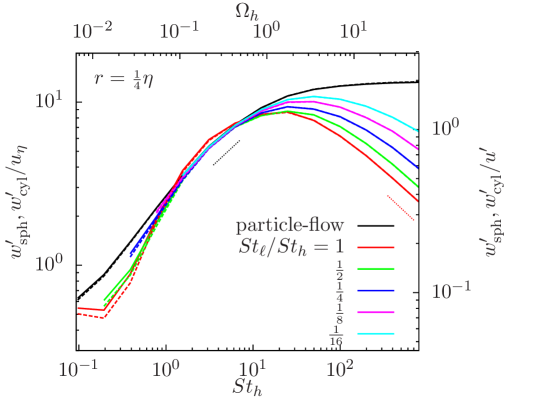
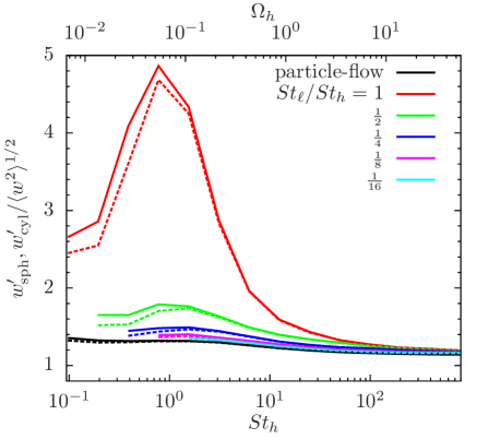
Figure 5.— Left panel: collision-rate weighted rms relative velocity in the spherical (solid, $w_{\rm sph}^{\prime}$) and cylindrical (dashed, $w_{\rm cyl}^{\prime}$) formulations at $r=\frac{1}{4}\eta$. Dotted line segments denote $St_{h}^{1/2}$ and $St_{h}^{-1/2}$ scalings. Right panel: ratios of $w_{\rm sph}^{\prime}$ and $w_{\rm cyl}^{\prime}$ to the unweighted rms.

Fig. 5 shows results for $w^{\prime}_{\rm sph}$ (solid) and $w^{\prime}_{\rm cyl}$ (dashed) measured at $r=\frac{1}{4}\eta$. The solid and dashed lines in Fig. 5 almost coincide. The equality of the weighted rms relative velocity in the two formulations was expected from the isotropy of ${\boldsymbol{w}}$. Slight differences ($\;\hbox to0.0pt{\lower 2.5pt\hbox{$\sim$}\hss}\raise 1.5pt\hbox{$<$}\;10\%$) are found at small $St_{h}$ and $f\;\hbox to0.0pt{\lower 2.5pt\hbox{$\sim$}\hss}\raise 1.5pt\hbox{$>$}\;1/2$, because, for these Stokes pairs, the assumption of perfect isotropy of ${\boldsymbol{w}}$ is not satisfied.

Interestingly, if the larger particle is in the inertial range, i.e., $\tau_{\eta}\;\hbox to0.0pt{\lower 2.5pt\hbox{$\sim$}\hss}\raise 1.5pt\hbox{$<$}\;\tau_{\rm p,h}\;\hbox to0.0pt{\lower 2.5pt\hbox{$\sim$}\hss}\raise 1.5pt\hbox{$<$}\;T_{\rm L}$, $w^{\prime}_{\rm cyl}$ and $w^{\prime}_{\rm sph}$ are almost independent of $f$, or the friction time, $\tau_{\rm p,l}$, of the smaller particle. In Paper II, we showed that the unweighted rms relative velocity, $\langle{\boldsymbol{w}}^{2}\rangle^{1/2}$, increases with decreasing $f$ because the generalized acceleration contribution to the relative velocity, corresponding to different responses of different particles to the flow velocity, increases with increasing fiction time difference (see Fig. 7 of Paper II). To understand the invariance of $w^{\prime}_{\rm sph,cyl}$ with $f$ for $St_{h}$ in the inertial range, it is helpful to compute the ratio of $w^{\prime}_{\rm sph,cyl}$ to the unweighted rms, $\langle{\boldsymbol{w}}^{2}\rangle^{1/2}$, which is shown in the right panel of Fig. 5. The ratio depends on the PDF shape of ${\boldsymbol{w}}$. Since $w^{\prime}_{\rm sph}$ and $w^{\prime}_{\rm cyl}$ correspond to higher (3rd) order statistics than the unweighted rms, the ratio $C_{32}\equiv w^{\prime}_{\rm sph,cyl}/\langle{\boldsymbol{w}}^{2}\rangle^{1/2}$ is larger if the PDF of ${\boldsymbol{w}}$ has fatter tails. In Paper III we found that, at a given $St_{h}$, the PDF shape of the relative velocity is the fattest for particles of equal size ($f=1$), and becomes continuously thinner as $f$ decreases. This explains why the ratios shown in the right panel increase as $f$ increases from 0 to 1. For $St_{h}$ in the inertial range, the larger ratio $C_{32}$ at larger $f$ happen to approximately cancel out the decrease of the unweighted rms, $\langle{\boldsymbol{w}}^{2}\rangle^{1/2}$, with increasing $f$ (see Fig. 7 of Paper II), leading to almost invariance of $w^{\prime}_{\rm sph,cyl}$ with $f$. This $f-$independence simplifies the estimate of the average collision energy of inertial-range particles. For $\tau_{\rm p,h}\simeq T_{\rm L}$, the average collision velocity for each collision is found to be $\simeq 1.3u^{\prime}$, independent of $f$. The collision velocity roughly follows a $St_{h}^{1/2}$ scaling for $St_{h}$ in the inertial range, which, however, needs to be verified by larger simulations with a broader inertial range.

For $St_{h}\;\hbox to0.0pt{\lower 2.5pt\hbox{$\sim$}\hss}\raise 1.5pt\hbox{$<$}\;1$ and $\tau_{\rm p,h}\;\hbox to0.0pt{\lower 2.5pt\hbox{$\sim$}\hss}\raise 1.5pt\hbox{$>$}\;T_{\rm L}$, the increase of $C_{32}$ with increasing $f$ is not sufficient to compensate the decrease of $\langle{\boldsymbol{w}}^{2}\rangle^{1/2}$, and the weighted rms is smaller at larger $f$. At $f=1$, the ratio $w^{\prime}_{\rm sph,cyl}/\langle{\boldsymbol{w}}^{2}\rangle^{1/2}$ strongly peaks at $St\simeq 1$, corresponding to the result of Paper III that the PDF is the fattest at $St\simeq 1$. As shown in Paper III, the PDF of ${\boldsymbol{w}}$ becomes nearly Gaussian for sufficiently large $\tau_{\rm p,h}$ ($\gg T_{\rm L}$), and, for a Gaussian distribution, it is easy to see that $w^{\prime}_{\rm cyl}/\langle{\boldsymbol{w}}^{2}\rangle^{1/2}=\sqrt{4/3}\simeq 1.15$. A ratio of 1.15 is actually observed at large $St_{h}$ in the right panel of Fig. 5. The right panel of Fig. 5 also suggests that using the unweighted rms $\langle{\boldsymbol{w}}^{2}\rangle^{1/2}$ significantly underestimates the average collision velocity per collision, especially for the collisions between particles of similar size with $St\simeq 1$.

For $f\leq{1/2}$, the measured rms velocity with collision-rate weighting converges at $r=\frac{1}{4}\eta$. The same is found for equal-size particles with $St\;\hbox to0.0pt{\lower 2.5pt\hbox{$\sim$}\hss}\raise 1.5pt\hbox{$>$}\;0.8$. However, complexities arise for smaller particles of equal size with $St\;\hbox to0.0pt{\lower 2.5pt\hbox{$\sim$}\hss}\raise 1.5pt\hbox{$<$}\;0.4$. For these particles, the weighted rms collision velocity has not reached convergence at $r=\frac{1}{4}\eta$, and a refinement is needed before it can be used in practical applications. In §3.3, in order to estimate the kernel in the $r\to 0$ limit, we attempted to isolate an $r-$independent kernel contribution by separating out the caustic pairs. However, we find that the method does not apply here to estimate the weighted rms collision velocity at $r\to 0$ or to obtain an $r-$independent contribution to the rms.

The idea of selecting the caustic pairs for small particles of equal size with $St\ll 1$ is to approximate the collision statistics at $r\to 0$ by the measured statistics of the relative velocity of particle pairs at a finite $r$ above a threshold. Although it was useful to obtain an $r-$independent kernel contribution, this approximation is not justified in general. When a threshold relative velocity is applied to select caustic pairs, the continuous pairs with low relative velocity are excluded, which pushes the rms relative velocity to higher values than the overall rms including all pairs at a given $r$. However, the rms collision velocity at $r\to 0$ is expected to be smaller than the overall rms at finite $r$, because the overall rms decreases with decreasing $r$. This suggests that the rms collision velocity of the caustic pairs does not correctly represent the rms in the $r\to 0$ limit. Thus, the relative velocity PDF excluding the continuous pairs at a finite $r$ is not equivalent to the PDF in the $r\to 0$ limit; instead it overestimates the collision velocity at $r\to 0$. We note that, when computing the rms collision velocity in simulations, Hubbard et al. (2012) proposed to count particle pairs with relative velocity above a threshold only. Based on the above discussion, there is uncertainty in the rms collision velocity measured this way as an estimate for $r\to 0$, and some care is needed when using such a method.

It turns out that isolating the caustic pairs from the continuous pairs does not help the convergence of the rms collision velocity. The threshold relative velocity is larger at larger $r$, as it is chosen to be linear with $r$ (see §3.3). It turns out that, with a stronger threshold, the weighted rms relative velocity of caustic pairs at a larger $r$ exceeds the overall rms by a larger amount than at smaller $r$. This means that the convergence of the rms relative velocity of caustic pairs is actually slower than the overall rms in the $r-$range ($\frac{1}{4}\eta\leq r\leq 1\eta$) explored here. In this range of $r$, the majority of particle pairs with $St\;\hbox to0.0pt{\lower 2.5pt\hbox{$\sim$}\hss}\raise 1.5pt\hbox{$<$}\;0.4$ belong to the continuous type, and the accuracy of approximating the actual statistics in the $r\to 0$ limit by the collision velocity of caustic pairs is poor. As $r$ decreases to a sufficiently small value so that most particle pairs are of the caustic type, the problem is expected to be less severe.

The above problem concerning the use of caustic pairs to approximate the $r\to 0$ statistics adds further uncertainty to the validity and accuracy of the criterion we adopted to isolate the caustic pairs, in addition to those already discussed in §3.3. Nevertheless, the classification of two types of particle pairs and the method used to splitting them based on theoretical models do offer physical insight to understand the $r-$dependence of the kernel in the $r$ range we explored. It is still possible that, despite this problem with the weighted rms collision velocity, our method to obtain the $r-$independent caustic kernel provides a reasonable approximation for the kernel at $r\to 0$ (see §3.3). Larger simulations that can measure the particle statistics at small scales are needed to test this possibility and to resolve the convergence issue.

We also note the red lines in the left panel of Fig. 5 rise slightly as $St$ decreases toward $St=0.1$. This behavior is unexpected, and is likely a numerical artifact, as the trajectory integration of $St=0.1$ particles, the smallest in our simulation, is the least accurate (see Papers I and II). The integration accuracy depends on the ratio of the simulation time step to the particle friction time, which is the largest for the smallest particles. This issue can be solved by future simulations with a better temporal resolution (see Paper II).

4.2. The Collision-Rate Weighted PDF

In Paper III, we computed the unweighted PDF of turbulence-induced relative velocity for all Stokes number pairs available in our simulation, and showed that the PDF of ${\boldsymbol{w}}$ is generically non-Gaussian, exhibiting fat tails. In that paper, we discussed in details the trend of non-Gaussianity with the particle friction times, and interpreted the results using the physical picture of the PP10 model. Here we examine the collision-rate weighted PDF of $|{\boldsymbol{w}}|$.

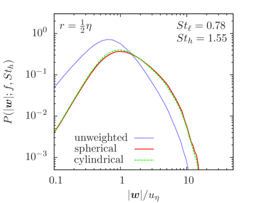
Figure 6.— PDFs of the 3D relative velocity amplitude for particles with $St_{\ell}=0.78$ and $St_{h}=1.55$ at a distance $r=\frac{1}{2}\eta$. The blue line shows the unweighted PDF, while the red and green lines correspond to the collision-rate weighted PDFs in the spherical and cylindrical formulations, respectively.

In Fig. 6, we illustrate the effect of collision-rate weighing using a Stokes number pair, $St_{\ell}=0.78$ and $St_{h}=1.55$, as an example. The dotted line shows the unweighted PDF, while the solid and dashed lines are the weighted PDFs, $P_{\rm sph}$ and $P_{\rm cyl}$, in the spherical and cylindrical formulations, respectively. Clearly, with the weighting factor, the PDF shows lower and higher probabilities at small and large collision speeds, respectively. As it favors large-velocity collisions, the collision-rate weighting increases the fraction of collisions leading to fragmentation, and reduces the probability of sticking. Consequently, the growth of dust particles would be more difficult than predicted by dust coagulation models that ignore the collision-rate weighting. The solid line and dashed lines almost coincide with each other. For this Stokes pair, the direction of ${\boldsymbol{w}}$ is nearly isotropic, and the weighted PDFs in the spherical and cylindrical formations are expected to be equal.

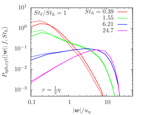
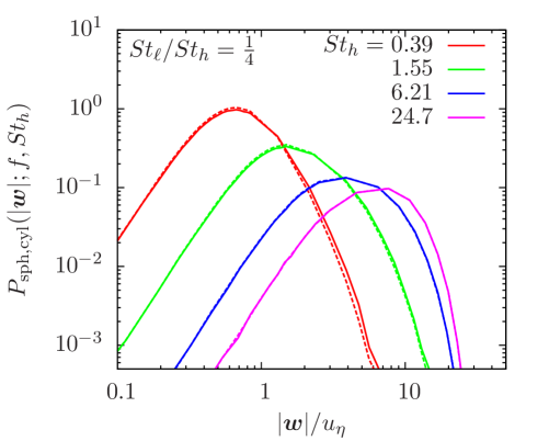
Figure 7.— Collision-rate weighted PDFs of the 3D amplitude, $|\boldsymbol{w}|$, in the spherical (solid) and cylindrical (dashed) formulations. The PDFs are measured at $r=\frac{1}{2}\eta$. The left panel plots the PDFs for particles of equal sizes, while the right panel shows results for a Stokes ratio of $f=\frac{1}{4}$.

Fig. 7 plots $P_{\rm sph}$ (solid lines ) and $P_{\rm cyl}$ (dashed lines) at more Stokes number pairs. The left and right panels show the measured PDFs for $f=1$ and $\frac{1}{4}$, respectively. The weighed PDFs in the two formulations are in good agreement for all the Stokes pairs. In cases where the two PDFs show differences, $P_{\rm cyl}$ has slightly higher and lower probabilities than $P_{\rm sph}$ at small and large $|{\boldsymbol{w}}|$, respectively. For $f=1$, the difference between $P_{\rm sph}$ and $P_{\rm cyl}$ is largest at $St=0.79$, and then decreases with increasing $St$. A comparison of the two panels shows that $P_{\rm sph}$ and $P_{\rm cyl}$ are in better agreement at smaller $f$. As shown in Paper II, the isotropy of ${\boldsymbol{w}}$ with respect to ${\boldsymbol{r}}$ improves with increasing $St$ or decreasing $f$.

The finding that $P_{\rm sph}\simeq P_{\rm cyl}$ at all Stokes number pairs suggests that either formulation can be used to determine the collision outcome in coagulation models for dust particle growth. The geometry assumed in the spherical formulation is physically more reasonable, but the weighted PDF in the cylindrical formulation appears to be more convenient, as it is directly related to the unweighted PDF as $|{\boldsymbol{w}}|P(|{\boldsymbol{w}}|)/\langle|{\boldsymbol{w}}|\rangle$. With this relation, one can easily determine the shape of $P_{\rm cyl}(|{\boldsymbol{w}}|)$ from the unweighted PDF presented in Paper III. It is expected that the trend of the shape of $P_{\rm cyl}(|{\boldsymbol{w}}|)$ (and hence $P_{\rm sph}$) with $f$ and $St_{h}$ would be similar to the unweighted PDFs discussed in Paper III. For example, if the shape of the unweighted PDF of $|{\boldsymbol{w}}|$ has a higher degree of non-Gaussianity, the weighted PDF would also have more probabilities at both left and right tails, corresponding to small and large collision velocities. We refer the interested reader to Paper III for a detailed discussion on the shape and the non-Gaussianity of the unweighted PDF as a function of $f$ and $St_{h}$.

An important application of the collision velocity PDF is to determine the outcome of dust particle collisions induced by turbulence in protoplanetary disks. In Paper III, we computed the fractions of collisions leading to sticking ($F_{\rm s}$), bouncing ($F_{\rm b}$) and fragmentation ($F_{\rm f}$) using typical disk and turbulence parameters at 1AU, and particular attention was given to the effect of the non-Gaussianity of the relative velocity PDF on the fractions. These fractions need to be incorporated in coagulation models for a realistic prediction of the dust size evolution. The calculation of the fractions was based on the PDF of $|{\boldsymbol{w}}|$ measured in our simulation using a weighting factor ($\propto|{\boldsymbol{w}}|$) from the cylindrical formulation. Several simplifying assumptions were used to extrapolate the measured PDFs in the simulated flow to the disk turbulence with much larger Reynolds number (see Paper III). In Appendix A, we compute $F_{\rm s}$, $F_{\rm b}$ and $F_{\rm f}$ from the weighted PDF, $P_{\rm sph}(|{\boldsymbol{w}}|)$, in the spherical formulation and compare the result with the cylindrical formulation. The calculation in Appendix A adopts the exact same parameters and assumptions as in Paper III. In Fig. 8 of Appendix A, we see that $F_{\rm s}$, $F_{\rm b}$ and $F_{\rm f}$ computed from the two formulations are consistent with each other, as expected from the agreement between $P_{\rm sph}$ and $P_{\rm cyl}$.

The spherical and cylindrical formulations yield very similar results for all the statistical quantities discussed so far, including the collision kernel, the collision-rate weighted rms and PDF of the 3D amplitude, $|\boldsymbol{w}|$, of the relative velocity, and the fractions of collisions leading to sticking, bouncing and fragmentation (Appendix A). All these quantities computed from the two formulations coincide with each other, except for small differences for Stokes pairs with $f$ close to 1 and $St_{h}\;\hbox to0.0pt{\lower 2.5pt\hbox{$\sim$}\hss}\raise 1.5pt\hbox{$<$}\;1$.

In Appendix B, we find an interesting difference between the two formulations concerning the collision-rate weighted PDFs of the radial and tangential components of ${\boldsymbol{w}}$. The statistics of the radial and tangential components is of interest because the collision outcome may depend on the angle at which the two particles collide. Appendix B shows that, in the spherical formulation, the weighted PDF, $P_{\rm sph}(|w_{\rm r}|)$, of the radial velocity amplitude of approaching particle pairs is very close to the PDF, $P_{\rm sph}(w_{\rm tt})$, of the total amplitude, $w_{\rm tt}$, of the two tangential components. This suggests that, on average, the collision energy in the radial direction is the same as the total tangential collision energy. On the other hand, the weighted radial PDF, $P_{\rm cyl}(|w_{\rm r}|)$, in the cylindrical formulation is found to almost coincide with the PDF, $P_{\rm cyl}(|w_{\rm t}|)$, of the amplitude, $|w_{\rm t}|$, of each single tangential component. Thus, each of the three directions provides equal amount of collision energy, which is in sharp contrast to the spherical formulation. As the weighting factor $\propto w_{\rm r}$, the spherical formulation gives more weight to collisions with larger radial relative speed. Consequently, it favors head-on collisions, and predicts more head-on collisions than the cylindrical formulation.

Different predictions for the weighted radial and tangential PDFs by the two formulations can be used to test which one is physically more realistic. The test requires directly measuring the PDFs of the radial and tangential relative speeds for particle pairs that are actually colliding. The direct measurement can be conducted using the method of Wang et al. (2000), which counts how many pairs of particles of given finite sizes get into contact during each small time step. Analyzing the statistics of the radial and tangential collision velocities of particle pairs in contact and comparing the results with the predictions by the two formulations would tell which formulation provides a better prescription for turbulence-induced collisions.

5. Discussion

A major result of our study is that, due to their stronger clustering, the collision kernel for particles of similar sizes in the inertial range is larger than between different particles. This is not captured by the collision formulation commonly used in dust coagulation models, as the clustering effect is neglected. We discuss the implication of this result on dust particle growth in protoplanetary disks. As an illustrating example, we consider collisions of silicate particles at 1 AU in a minimum mass solar nebula. In the example, we use the same disk and turbulence parameters as in Paper III, to which we refer the reader for details.

As the particle size grows to $\simeq 1$ mm at 1AU, the typical collision velocity induced by turbulence exceeds the bouncing threshold ($\simeq 5$ cm s^-1), and the collision outcome starts to be dominated by bouncing rather than sticking (Fig. 8 in Appendix B; see also Paper III). If the probability distribution of the collision velocity is neglected, the growth of dust particles would stall at the millimeter size, a problem known as the bouncing barrier for planetesimal formation (Zsom et al. 2010, Gültler et al. 2010). The friction time, $\tau_{\rm p}$, of millimeter-size particles is close to the Kolmogorov time at 1 AU, meaning that the bouncing barrier starts once the particles reach the inertial range of the flow.

Recent studies by Windmark et al. (2012) and Garaud et al. (2013) showed that the bouncing barrier may be overcome if the probability distribution of the collision velocity is taken into account. With a collision velocity distribution, there is always a finite probability of low-velocity collisions leading to sticking, even if the typical collision velocity is already above the bouncing threshold. If, by “luck”, a particle experiences low-velocity collisions continuously, it may grow significantly past the millimeter size. In Paper III, we showed that, unlike the assumption of Gaussian distribution made by Windmark et al. (2012) and Garaud et al. (2013), the PDF of the collision velocity ${\boldsymbol{w}}$ is highly non-Gaussian, and accounting for the non-Gaussianity gives significantly higher probabilities of sticking, further alleviating the bouncing barrier (see Paper III). In Appendix B, we computed the probabilities of sticking, bouncing and fragmentation as a function of the particle size using both spherical and cylindrical formulations.

A “lucky” particle that grows past the bouncing barrier and reaches the fragmentation barrier around decimeter size can further grow by the so-called mass transfer mechanism (Windmark 2012). In this mechanism, a large particle acquires mass when colliding with much smaller particles. The collision breaks up the small particle, and some of its fragments stay on the large particle. The large particle can thus grow beyond the fragmentation barrier and toward the planetesimal size by continuously sweeping up mass of small particles (Windmark 2012). The mass transfer mechanism occurs only when the size ratio of the two particles is sufficiently large, and thus relies on the formation of large “seed” by coagulational growth in between the bouncing and fragmentation barriers.

Windmark et al. (2012) found that, due to the small sticking probability, particle growth from the bouncing barrier size toward the fragmentation barrier is very slow with a timescale of $10^{4}$ yr. In the present work, we have shown that turbulent clustering increases the particle collision rate, and thus can accelerate particle growth in between the two barriers, further alleviating the bouncing barrier. The acceleration is the most efficient for particles of similar sizes, for which the clustering effect peaks and the collision kernel is the largest. Interestingly, for collisions between particles of similar sizes, the probability of sticking is the largest. As shown in Fig. 8 in Appendix B (see also Fig. 16 in Paper III), the decay of the sticking probability with increasing size, $a_{\rm p,h}$, of the larger particle is the slowest at $f=1$, and is significantly more rapid as $f$ decreases toward 0. These suggest that the effect of clustering preferentially increases the rate of collisions that have a higher probability of sticking. In other words, the clustering effect increases not only the overall collision rate, but also the overall fraction of collisions leading to sticking. Therefore, the acceleration of the particle growth by the clustering effect past the bouncing barrier is likely quite efficient. The above discussion also indicates that particle growth between the bouncing and fragmentation barriers would occur mainly through collisions between particles of similar sizes.

The effect of turbulent clustering on dust particle growth at 1 AU can be summarized as follows. When reaching millimeter size, the particle friction time enters the inertial range of the flow, and turbulent clustering starts to significantly increase the collision kernel. Meanwhile, the collision outcome is dominated by bouncing, and the particle growth beyond the bouncing barrier relies on the finite but decaying probabilities of low collision velocity that allows sticking. Turbulent clustering helps accelerate the particle growth past the bouncing barrier, and, in particular, it preferentially enhances the collision rate between similar-size particles, which have a higher sticking probability. Accounting for the effect of clustering would thus help alleviate the bouncing barrier and accelerate the formation of large seed particles that can further grow beyond the fragmentation barrier by the sweep up mechanism.

A quantitative estimate for how fast turbulent clustering can accelerate the particle growth requires future studies to examine the Reynolds number ($Re$) dependence, which is needed to extrapolate the collision statistics in our flow to protoplanetary turbulence. Fig. 1 shows that clustering effect is strongest at $St\simeq 1$ (corresponding to $\simeq 1$mm at 1AU), and it can amplify the collision rate of equal-size particles with $St\simeq 1$ by an order of magnitude. The acceleration would be faster if the radial distribution function, $g$, has a significant $Re-$dependence. Note that in our simulation the clustering effect significantly decreases as $St$ increases above 1 and already becomes weak for $St=6.21$ particles in the inertial range (see Fig. 1). How much turbulent clustering can accelerate the collision rate of inertial-range particles of similar sizes in a realistic disk flow depends on the Reynolds number dependence of the RDF (see §3.5). A refined dust coagulation model that incorporates the clustering effect as well as the non-Gaussianity of the collision velocity is needed to give a conclusive answer for how and how fast dust particles grow in between the bouncing and fragmentation barriers. We point out that turbulent clustering may not be helpful for the fast drift problem of meter-size particles. The friction timescale of these large particles is close to the large eddy time in the disk, and the effect of turbulent clustering is expected to be weak, and would thus not help speed up the collisions of these particles.

6. Summary and Conclusions

Motivated by the problem of dust particle growth in protoplanetary disks, we studied the collision statistics of inertial particles suspended in turbulent flows. Using a numerical simulation, we evaluated the collision kernel as a function of the friction times of two particles of arbitrary sizes, accounting for the effects of turbulent clustering and turbulence-induced collision velocity. We also computed the statistics of the collision velocity using a collision-rate weighting factor to account for the higher collision frequency for particle pairs with larger relative speed. Below we list the main conclusions of this study.

1. If the friction time, $\tau_{\rm p,h}$, of the larger particle is below the Kolmogorov time, $\tau_{\eta}$, or above the Lagrangian correlation time, $T_{\rm L}$, the collision kernel per unit cross section is found to be larger at smaller Stokes (or friction time) ratio $f$ ($\equiv St_{\ell}/St_{h}$). This is because, at given $\tau_{\rm p,h}$, the particle relative velocity increases with decreasing $f$, due to the increase of a contribution, named the acceleration contribution, corresponding to different responses of particles of different sizes to the flow velocity. On the other hand, for $\tau_{\rm p,h}$ in the inertial range ($\tau_{\eta}\;\hbox to0.0pt{\lower 2.5pt\hbox{$\sim$}\hss}\raise 1.5pt\hbox{$<$}\;\tau_{\rm p,h}\;\hbox to0.0pt{\lower 2.5pt\hbox{$\sim$}\hss}\raise 1.5pt\hbox{$<$}\;T_{\rm L}$), the kernel per unit cross section increases with increasing $f$ and is the largest at $f=1$, due to the effect of turbulent clustering, which peaks for equal-size particles. Thus, as the typical particle friction time, $\tau_{\rm p}$, enters the inertial range of the flow, collisions between similar particles become more frequent than between particles of different sizes. If the friction time, $\tau_{\rm p,h}$, of the larger particle is close to $T_{\rm L}$, the kernel per unit cross section is about equal to the 1D rms flow velocity, $u^{\prime}$, independent of $f$ or the friction time, $\tau_{\rm p,l}$, of the smaller particle.

2. The kernel formula commonly used in dust coagulation models neglects the effect of turbulent clustering and uses the rms relative velocity ($\langle w^{2}\rangle^{1/2}$) instead of the mean relative speeds ($\langle|w_{\rm r}|\rangle$ or $\langle|{\boldsymbol{w}}|\rangle$). The former underestimates the collision rate, while the latter tends to overestimate it, as the rms relative velocity is larger than the mean. For particles of similar sizes with $St_{\rm h}$ in the inertial range, clustering is strong and more than compensates the latter effect. Neglecting clustering would thus significantly underestimate the collision rate of particles of similar sizes (${\boldsymbol{f}\simeq 1}$), especially at $St_{h}\simeq 1$.

3. We analyzed the collision-rate weighted statistics for the particle relative velocity, ${\boldsymbol{w}}$. With a collision-rate weighting factor, the rms relative velocity measures the average collision energy per collision. The weighting factor is proportional to the particle relative velocity ($w_{\rm r}$ or $|{\boldsymbol{w}}|$), and favors collisions with larger collision velocity, leading to larger rms values than without weighting. The weighted rms corresponds to the 3rd order statistics, and the enhancement over the unweighted rms depends on the PDF shape of ${\boldsymbol{w}}$. The ratio of the weighted rms to the unweighted one increases as $f$ increases toward 1, due to the fatter PDF shape at larger $f$. The ratio is the largest for particles of equal sizes ($f=1$), and ignoring the collision-rate weighting would significantly underestimate the average collision energy between particles of similar sizes. For $\tau_{\rm p,h}$ in the inertial range, the weighted rms is independent of the size of the smaller particle, and scales with $\tau_{\rm p,h}$ roughly as $\tau_{\rm p,h}^{1/2}$ for any $f$. For particles with $\tau_{\rm p,h}\simeq T_{\rm L}$ in our simulation, the weighted rms collision velocity is approximately $\simeq 1.3u^{\prime}$ at any $f$.

   As more weight is given to collisions with larger relative velocity, the weighted distribution of the 3D amplitude, $|{\boldsymbol{w}}|$, of the collision velocity shows higher (lower) probabilities at large (small) collision velocities. Therefore, ignoring the collision-rate weighting would overestimate (or underestimate) the fraction of collisions resulting in sticking (or fragmentation).

4. We argued that the effect of turbulent clustering helps alleviate the bouncing barrier for planetesimal formation. As it increases the probability of finding colliding neighbors, the spatial clustering of dust particles enhances the collision kernel, and can accelerate the particle growth past the bouncing barrier. The acceleration is the fastest for particles of similar sizes in the inertial range, and, considering that the probability of sticking is also the largest for particles of similar sizes, the effect of clustering not only increases the overall collision rate, but also the overall fraction of collisions leading to sticking. The acceleration of particle growth by turbulent clustering beyond the bouncing barrier is thus expected to be efficient.

5. We compared two kernel formulations based on spherical and cylindrical geometries. The two formulations give consistent results for the collision rate, the collision-rate weighted rms and PDF of $|{\boldsymbol{w}}|$. We showed that these quantities computed from the two formulations are expected to be exactly equal, if the direction of the relative velocity, $\boldsymbol{w}$, of two particles is statistically isotropic with respect to their separation, ${\boldsymbol{r}}$. For small particles of similar sizes, ${\boldsymbol{w}}$ is not perfectly isotropic, and slight differences between the two formulations are observed at $f\;\hbox to0.0pt{\lower 2.5pt\hbox{$\sim$}\hss}\raise 1.5pt\hbox{$>$}\;\frac{1}{2}$ and $St_{h}\;\hbox to0.0pt{\lower 2.5pt\hbox{$\sim$}\hss}\raise 1.5pt\hbox{$<$}\;1$. Isotropy of $\boldsymbol{w}$ improves with increasing $St_{h}$ or decreasing $f$, leading to the equality of the collision kernel and collision-rate weighted PDFs of $|\boldsymbol{w}|$ in the two formulations. The two formulations also give similar estimates for the fractions of collisions resulting in sticking, bouncing and fragmentation.

   An interesting difference between the two formulations is found concerning the weighted PDFs of the radial and tangential components of ${\boldsymbol{w}}$. In the spherical formulation, the weighted PDF of the radial component almost coincides with that of the total tangential amplitude, while in the cylindrical formulation the weighted radial PDF is about equal to the distribution of each single tangential component. As its weighting factor favors collisions with larger radial collision speed, the spherical formulation predicts more head-on collisions than the cylindrical formulation. This difference provides a unique test for the two kernel prescriptions with different geometries.

Although the present study draws significant conclusions on the statistics of dust particle collisions induced by turbulence, several important questions remain to be answered by future work. First, the Reynolds-number dependence of the clustering effect and the collision kernel is currently unknown and needs to be examined using simulations at higher resolutions. Application of the measured statistics in our simulation to protoplanetary disks requires an extrapolation to high Reynolds numbers appropriate for the disk conditions.

Second, our simulation data provides accurate statistical measurements only at particle distances $r\;\hbox to0.0pt{\lower 2.5pt\hbox{$\sim$}\hss}\raise 1.5pt\hbox{$>$}\;\frac{1}{4}$, but the collision kernel for small particles of equal-size with $St\;\hbox to0.0pt{\lower 2.5pt\hbox{$\sim$}\hss}\raise 1.5pt\hbox{$<$}\;1$ does not converge at $r=\frac{1}{4}\eta$. We have discussed some uncertainties in our method to isolate an $r-$ independent kernel contribution by separating out the caustic particle pairs. Also, the collision-rate weighted rms relative velocity for small particles of the same size has not reached convergence at $r\simeq\frac{1}{4}\eta$. Simulations with a larger number of particles that allow measurements at smaller $r$ would help resolve these issues.

Another interesting question is whether and how the collision statistics of particles with friction time that couples to the flow driving scales is affected by the specific driving mechanism. A set of numerical simulations with different driving schemes would help clarify the possible effects of the driving force.

Finally, to evaluate the accuracy of the collision rate commonly used in the dust coagulation models, we need to carefully test the prediction of the model by Völk et al. (1980) and its successors for the (unweighted) rms relative velocity. We will conduct a systematic test of the Völk-type models against our simulation data in a future paper.

Appendix A Comparing Collision Outcomes in Spherical and Cylindrical Formulations

In Paper III, we computed the fractions, $F_{\rm s}$, $F_{\rm b}$, and $F_{\rm f}$, of collisions leading to sticking, bouncing and fragmentation as a function of the dust particle sizes in protoplanetary disks, using the relative velocity PDF measured in our simulation. In the calculation, we adopted a minimum mass solar nebula and considered particle collisions at 1AU as an illustrating example. Turbulence condition in the disk was specified using the prescription of Cuzzi et al. (2001) with the Shakura-Sunyaev parameter $\alpha_{\rm t}$ set to $10^{-4}$. Due to the limited resolution, the inertial range of our simulated flow is very short, and we made a few assumptions to extrapolate the measured PDFs to the disk flow with a much larger Reynolds number. For example, we set the shape of the PDF for all inertial-range particles in a real disk to be same as the measured distribution of $St=6.21$ particles, the only particle species that definitely lies in the inertial range of the simulated flow. Clearly, this is a strong simplification, and an accurate treatment needs the Reynolds-number dependence of the PDF, which is currently unknown. We assumed that, for collisions of silicate particles, bouncing and fragmentation occur as the collision velocity exceeds the threshold values of 5 cm s^-1 and 1 m s^-1, respectively. We refer the reader to Paper III for a detailed description of the assumptions and parameters used in the calculation.

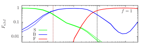
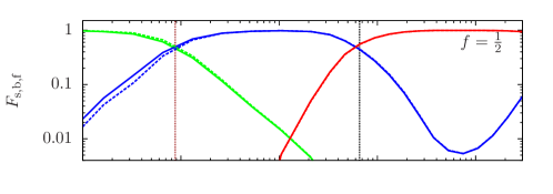
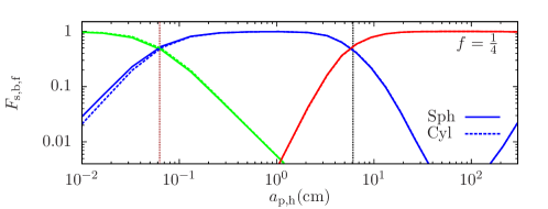
Figure 8.— Sticking (green), bouncing (blue) and fragmentation (red) fractions as a function of the size, $a_{\rm{p,h}}$, of the larger particle. The three panels show fixed Stokes number ratios at $f=1$, $\frac{1}{2}$, and $\frac{1}{4}$. Vertical brown and black dotted lines correspond to critical $a_{\rm{p,h}}$ at which the unweighted rms relative velocity is equal to bouncing and fragmentation thresholds, respectively. Solid and dashed lines are computed from the weighted PDFs at a particle distance of $r=\frac{1}{2}\eta$ using the spherical and cylindrical formulations, respectively.

The calculation of $F_{\rm s}$, $F_{\rm b}$, and $F_{\rm f}$ in Paper III was based on the measured PDF of the 3D amplitude, $|{\boldsymbol{w}}|$, using a cylindrical weighting factor $\propto|{\boldsymbol{w}}|$. Here, we compare the estimates from the spherical and cylindrical formulations. Fig. 8 shows $F_{\rm s}$ (green), $F_{\rm b}$ (blue), and $F_{\rm f}$ (red), as a function of the size, $a_{\rm p,h}$, of the larger particle. The solid and dashed lines are calculated from the wighted PDFs, $P_{\rm sph}$ and $P_{\rm cyl}$, at a particle distance $r=\frac{1}{2}\eta$. As mentioned in Paper III, it is desirable to use PDFs at smaller $r$, which, however, cannot be measured at high accuracy in our simulation. The figure is plot in the same way as Fig. 16 of Paper III. The three panels from top to bottom show the results for Stokes number ratios of $f=1$, $\frac{1}{2}$, and $\frac{1}{4}$, respectively. The dashed lines here correspond to the solid lines in Fig. 16 of Paper III.

The vertical brown and black dotted lines in each panel mark the sizes of the larger particle, at which the unweighted rms relative velocity reaches the bouncing and fragmentation thresholds, respectively. In dust coagulation models that ignore the collision velocity distribution, it was assumed that the collision outcome makes a sharp transition from sticking to bouncing and to fragmentation at the brown and dotted lines, respectively. Including the collision velocity distribution makes the transitions gradual because with a distribution there is always a finite probability of finding low (or high) collision velocities, even if the rms relative velocity is already above (or still below) the bouncing or fragmentation thresholds (see Windmark 2012, Garaud et al. 2013).

In Paper III, we showed that the distribution of ${\boldsymbol{w}}$ is non-Gaussian, and accounting for the non-Gaussianity leads to more gradual transitions. In particular, the decay of the sticking fraction with increasing $a_{\rm p,h}$ is significantly slower than the estimate based on the assumption of a Gaussian distribution (see Fig. 16 of Paper III). We therefore argued that incorporating the non-Gaussianity of the collision velocity is helpful for the particle growth and further alleviates the problem of the bouncing barrier. A comparison of the three panels shows that the sticking fraction is more persistent at larger $f$. This corresponds to the higher degree of non-Gaussianity of the PDF for particles of similar sizes. A detailed discussion on the behavior of the fractions with $f$ and $St_{\rm h}$ was given in Paper III.

The solid and dashed lines for the spherical and cylindrical formulations almost coincide, consistent with the agreement of $P_{\rm sph}$ and $P_{\rm cyl}$ found in §4.2. This suggests that either formulation can be used to estimate the collision outcome. The slight difference between the solid and dashed lines corresponds to the difference between $P_{\rm sph}$ and $P_{\rm cyl}$ shown in Fig. 7. The difference decreases with decreasing $f$ because the direction of ${\boldsymbol{w}}$ is more isotropic at smaller $f$ and the agreement between $P_{\rm sph}$ and $P_{\rm cyl}$ improves (see Fig. 7).

Appendix B Collision-rate Weighted PDFs in Radial and Tangential Directions

In this appendix, we consider the radial and tangential components of the relative velocity. An analysis of the radial and tangential relative speeds is of interest, as the collision outcome may depend on the angle at which two particles collide. We decompose ${\boldsymbol{w}}$ to a radial component, $w_{\rm r}$, and two tangential components, $w_{\rm t1}$ and $w_{\rm t2}$. In an isotropic flow, $w_{\rm t1}$ and $w_{\rm t2}$ are statistically equivalent, and we use $w_{\rm t}$ to represent the statistics of one tangential component. In Papers I, II and III, we studied the statistics of $w_{\rm r}$ and $w_{\rm t}$ without collision-rate weighting. Here we examine the collision-rate weighted PDFs of $w_{\rm r}$ and $w_{\rm t}$. We also analyze the total tangential amplitude, $w_{\rm tt}$, defined as $w_{\rm tt}\equiv(w_{\rm t1}^{2}+w_{\rm t2}^{2})^{1/2}$.

In the spherical formulation, the weighted distribution, $P_{\rm sph}(|w_{\rm r}|)$, for the radial amplitude, $|w_{\rm r}|$, of approaching particle pairs ($w_{\rm r}\leq 0$) is related to the left (negative) wing of the unweighted radial PDF, $P(w_{\rm r})$, by $P_{\rm sph}(|w_{\rm r}|)\propto|w_{\rm r}|P(-|w_{\rm r}|)$. In terms of the PDF, $P_{\rm v}({\boldsymbol{w}})$, of the vector ${\boldsymbol{w}}$, we have,

$$P_{\rm sph}(|w_{\rm r}|)=-\frac{1}{N}\int\limits_{-\infty}^{0}w^{\prime}_{\rm r}dw^{\prime}_{\rm r}\int\limits_{-\infty}^{\infty}dw^{\prime}_{\rm t1}\int\limits_{-\infty}^{\infty}dw^{\prime}_{\rm t2}\delta(|w_{\rm r}|+w^{\prime}_{\rm r})P_{\rm v}(w^{\prime}_{\rm r},w^{\prime}_{\rm t1},w^{\prime}_{\rm t2}),$$ (B1)

where $N=-\int_{-\infty}^{0}w_{\rm r}P(w_{\rm r})dw_{\rm r}$ normalizes the total probability to unity. The weighted PDF for the total tangential amplitude, $w_{\rm tt}$, is given by,

$$P_{\rm sph}(w_{\rm tt})=-\frac{1}{N}\int\limits_{-\infty}^{0}w^{\prime}_{\rm r}dw^{\prime}_{\rm r}\int\limits_{-\infty}^{\infty}dw^{\prime}_{\rm t1}\int\limits_{-\infty}^{\infty}dw^{\prime}_{\rm t2}\delta(w_{\rm tt}-(w^{\prime 2}_{\rm t1}+w^{\prime 2}_{\rm t2})^{1/2})P_{\rm v}(w^{\prime}_{\rm r},w^{\prime}_{\rm t1},w^{\prime}_{\rm t2}).$$ (B2)

Again, it is useful to consider the case where ${\boldsymbol{w}}$ is isotropic and $P_{\rm v}(w_{\rm r},w_{\rm t1},w_{\rm t2})=P_{\rm v}(|{\boldsymbol{w}}|)=P_{\rm v}((w_{\rm r}^{2}+w_{\rm t1}^{2}+w_{\rm t2}^{2})^{1/2})$. In this case, integration of eqs. (B1) and (B2) gives,

$$P_{\rm sph}(|w_{\rm r}|)=\frac{2\pi}{N}|w_{\rm r}|\int_{|w_{\rm r}|}^{\infty}|{\boldsymbol{w}}|P_{\rm v}(|{\boldsymbol{w}}|)d|{\boldsymbol{w}}|,\hskip 5.69046pt{\rm and}\hskip 5.69046ptP_{\rm sph}(w_{\rm tt})=\frac{2\pi}{N}w_{\rm tt}\int_{w_{\rm tt}}^{\infty}|{\boldsymbol{w}}|P_{\rm v}(|{\boldsymbol{w}}|)d|{\boldsymbol{w}}|.$$ (B3)

Therefore, if the direction of ${\boldsymbol{w}}$ is uniformly distributed with respect to ${\boldsymbol{r}}$, the collision-rate weighted PDF of the radial component is identical to that of the total tangential amplitude.

In the left panel of Fig. 9, we plot $P_{\rm sph}(|w_{\rm r}|)$ and $P_{\rm sph}(w_{\rm tt})$ in the spherical formulation for particles of equal sizes. The figure shows that the weighted PDFs of $|w_{\rm r}|$ and $w_{\rm tt}$ almost coincide for all $St$. Slight difference occurs only at small $St\;\hbox to0.0pt{\lower 2.5pt\hbox{$\sim$}\hss}\raise 1.5pt\hbox{$<$}\;1$, where the direction of ${\boldsymbol{w}}$ is not perfectly isotropic (see Paper I). As $St$ increases above 1, the direction of ${\boldsymbol{w}}$ becomes isotropic, and the difference between $P_{\rm sph}(|w_{\rm r}|)$ and $P_{\rm sph}(w_{\rm tt}$) disappears. The isotropy of ${\boldsymbol{w}}$ also increases with decreasing Stokes ratio $f$ or decreasing particle distance, $r$ (Paper II). Therefore, a better agreement between $P_{\rm sph}(|w_{\rm r}|)$ and $P_{\rm sph}(w_{\rm tt})$ is observed at smaller $f$ and/or smaller $r$ (not shown).

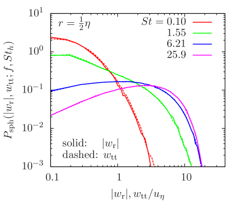
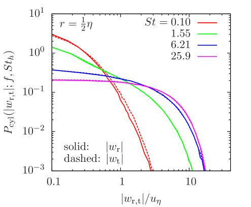
Figure 9.— Left panel: Collision-rate weighted PDFs for the amplitude, $|w_{\rm r}|$, of the radial relative speed and the total tangential amplitude, $w_{\rm tt}$ for equal-size particles with different $St$. Right panel: the weighted PDFs of the amplitudes of the radial component, $|w_{\rm r}|$, and of a single tangential component in the cylindrical formulations. In both panels, the PDFs are measured at $r=\frac{1}{2}\eta$.

The near coincidence of $P_{\rm sph}(|w_{\rm r}|)$ and $P_{\rm sph}(w_{\rm tt})$ indicates that the weighted rms of the radial collision velocity is about equal to that of the total tangential amplitude, or equivalently, on average, the collision energy in the radial direction is the same as the total tangential energy. This is in contrast to the case without collision-rate weighting, where the rms of the radial relative speed t is equal to that of each tangential component, expect for slight differences for small particles of similar sizes with $St_{h}\;\hbox to0.0pt{\lower 2.5pt\hbox{$\sim$}\hss}\raise 1.5pt\hbox{$<$}\;1$ (see Papers I and II).

As the collision rate is proportional to $|w_{\rm r}|$ in the spherical formulation, collisions with larger radial relative velocity are given more weight. The finding that the weighted rms and PDF of the radial component is the same as the total tangential amplitude suggests a higher frequency of head-on collisions than if the collision-rate weighting is ignored. In other words, the collision-rate weighting in the spherical formulation favors head-on collisions. This may have important implications for the collisional growth of dust particles if the collision outcome has a significant dependence on the colliding angle.

We also computed the weighted PDFs of the radial and tangential components in the cylindrical formulation. Unlike the case of the spherical formulation, the weighting factor ($\propto|{\boldsymbol{w}}|$) in the cylindrical formulation does not favor a particular direction. Thus, if the direction of ${\boldsymbol{w}}$ is statistically isotropic, the weighted PDFs of the three components of the relative velocity are expected to the same. The weighted PDF of the radial amplitude, $|w_{\rm r}|$, in the cylindrical formulation can be defined as $P_{\rm cyl}(|w_{\rm r}|)=\frac{1}{\langle|{\boldsymbol{w}}|\rangle}\int_{-\infty}^{\infty}dw^{\prime}_{\rm r}\int_{-\infty}^{\infty}dw^{\prime}_{\rm t1}\int_{-\infty}^{\infty}dw^{\prime}_{\rm t2}\delta(|w_{\rm r}|-|w^{\prime}_{\rm r}|)|{\boldsymbol{w}}|P_{\rm v}(w^{\prime}_{\rm r},w^{\prime}_{\rm t1},w^{\prime}_{\rm t2})$, and, assuming isotropy for the direction of ${\boldsymbol{w}}$, we find $P_{\rm cyl}(|w_{\rm r}|)=4\pi\int_{|w_{\rm r}|}^{\infty}|{\boldsymbol{w}}|^{2}P_{\rm v}(|{\boldsymbol{w}}|)d|{\boldsymbol{w}}|/\langle|{\boldsymbol{w}}|\rangle$. Similarly, it can be shown that the weighted PDF for the amplitude of one tangential component, $w_{\rm t}$, has the same form, $P_{\rm cyl}(|w_{\rm t}|)=4\pi\int_{|w_{\rm t}|}^{\infty}|{\boldsymbol{w}}|^{2}P_{\rm v}(|{\boldsymbol{w}}|)d|{\boldsymbol{w}}|/\langle|{\boldsymbol{w}}|\rangle$. In the right panel of Fig. 9, we plot the weighted PDFs of $|w_{\rm r}|$ (solid lines) and $|w_{\rm t}|$ (dashed lines) for particles of equal size in the cylindrical formulation. As expected, $P_{\rm cyl}(|w_{\rm r}|)$ and $P_{\rm cyl}(|w_{\rm t}|)$ coincide at $St\;\hbox to0.0pt{\lower 2.5pt\hbox{$\sim$}\hss}\raise 1.5pt\hbox{$>$}\;1$, where the direction of ${\boldsymbol{w}}$ is isotropic. At $St\;\hbox to0.0pt{\lower 2.5pt\hbox{$\sim$}\hss}\raise 1.5pt\hbox{$<$}\;1$, the tail of $P_{\rm cyl}(|w_{\rm t}|)$ is slightly broader than $P_{\rm cyl}(|w_{\rm r}|)$, and, correspondingly, the weighted rms relative velocity in a tangential direction is slightly larger than in the radial direction. The equality of $P_{\rm cyl}(|w_{\rm r}|)$ and $P_{\rm cyl}(|w_{\rm t}|)$ also improves with decreasing $f$ and/or decreasing $r$. A comparison of the solid lines in the left and right panels of Fig. 9 shows that the two formulations give different estimates for the weighted radial PDFs.

The near equality of $P_{\rm cyl}(|w_{\rm r}|)$ and $P_{\rm cyl}(|w_{\rm t}|)$ in the cylindrical formulation suggests that, on average, each of three directions provides the same amount of collision energy. Thus, the total collision energy in the two tangential directions is twice larger than in the radial direction. This is different from the spherical formulation, where the collision energy in the radial direction is about equal to the sum from the two tangential components. The spherical formulation favors collisions with larger radial relative speed and predicts more head-on collisions than the cylindrical formulation.

In summary, we find an interesting difference between the two kernel formulations. In the spherical formulation, the weighted PDF of the radial component almost coincides with that of the total tangential amplitude, while in the cylindrical formulation the weighted radial PDF is nearly equal to the distribution of each single tangential component. Note that the two formulations give similar estimates for all the quantities discussed in the text and in Appendix A, including the collision kernel, the collision-rate weighted PDF of $|{\boldsymbol{w}}|$, and the fractions of collisions leading to sticking, bouncing and fragmentation. Thus, the difference in the predictions for the weighted radial and tangential PDFs provides a useful tool to test the two formulations. To carry out the test, one can directly measure the collision statistics by considering the finite particle size (instead of assuming point particles) and counting how many pairs of particles get into contact during each infinitesimal time interval. Analyzing the radial and tangential relative velocities of these particle pairs in contact would tell which formulation is a better prescription for turbulence-induced collisions. We defer the direct measurements of the collision statistics to a future work.

References

- (1)
- (2) Blum, J. & Wurm, G. 2008, ARAA, 46, 21
- (3) Brandenburg, A., & Dobler, W. 2002, Computer Physics Communications, 147, 471
- (4) Cencini, M., Bec. J., Biferale, L., Boffetta, G., Celani, A., Lanotte, A. S., Musacchio, S. & Toschi, F. 2006, Journal of Turbulence, 7, N36
- (5) Chiang, E. & Youdin 2010, AREPS, 38493
- (6) Collins, L. R. & Keswani, A. 2004 New J. Phys. 6, 119
- (7) Cuzzi, J. N. & Hogan R. C. 2003, Icarus,164, 127
- (8) Cuzzi, J. N., Hogan, R. C., Paque, J. M., & Dobrovolskis, A. R. 2001, ApJ, 546, 496
- (9) Chun, J., Koch, D. L., Rani, S.L., Ahluwalia, A. & Collons, L. 2005, J. Fluid Mech., 536, 219
- (10) Garaud, P., Meru, F., Galvagni, M., & Olczak, C. 2013, ApJ, 764, 146
- (11) Falkovich, G., Fouxon, A., & Stepanov, M. G. 2002, Nature, 419, 151
- (12) Falkovich, G., & Pumir, A. 2004, Physics of Fluids, 16, L47
- (13) Falkovich, G. & Pumir, A. 2007, J. Atmos. Sci. 64, 4497
- (14) Güttler, C., Blum, J., Zsom, A., Ormel, C. W.,& Dullemond, C. P. 2010, A&A, 513, A56
- (15) Gustavsson, K. & Mehlig, B. 2011, Phys. Rev. E, 84, 045304(R)
- (16) Hogan, R. C., & Cuzzi, J. N. 2001, Phys. Fluids, 13, 2938
- (17) Hubbard, A. 2012, MNRAS, 426, 784
- (18) Hubbard, A. 2013, MNRAS, 432, 1274
- (19) Johansen, A., Andersen, A. C., & Brandenburg, A. 2004, A&A, 417, 361
- (20) Markiewicz, W. J., Mizuno, H., & Völk, H. J. 1991, A&A, 242, 286
- (21) Maxey, M. R. 1987, J. Fluid Mech., 174, 441
- (22) Monin, A. S. & Yaglom, A. M. 1975, Statistical Fluid Mechanics: Mechanics of Turbulence, vol. 2. MIT press.
- (23) Ormel, C. W., & Cuzzi, J. N. 2007, A&A, 466, 413
- (24) Padoan, P., Jimenez, R., Nordlund, Å., & Boldyrev, S. 2004, Physical Review Letters, 92, 191102
- (25) Pan, L. & Padoan, P. 2010, J. of Fluid Mech., 661, 73 (PP10)
- (26) Pan, L. & Padoan, P. 2013, ApJ, 776, 12 (Paper I)
- (27) Pan, L. & Padoan, P., & Scalo, J. 2014a, ApJ, 791, 48 (Paper II)
- (28) Pan, L. & Padoan, P., & Scalo, J. 2014b, ApJ, 792, 69 (Paper III)
- (29) Pan, L., Padoan, P.. Scalo, J., Kritsuk, A. G., & Norman, M. L. 2011, ApJ, 740, 21
- (30) Pan, L. & Scannapieco, E. 2011, Phys. Rev. E, 2011, 83, 045302(R)
- (31) Porter, D. , Pouquet, A., & Woodward, P. 2002, Phys. Rev. E 66, 026301
- (32) Saffman, P. G. & Turner, J. S.1956 J. Fluid Mech., 1, 16
- (33) Squires, K. D., & Eaton, J. K. 1991, Phys. Fluids, 3, 1169
- (34) Völk, H. J., Jones, F. C., Morfill, G. E.& Roeser, S. 1980, A&A, 85, 316–325
- (35) Wang, L.-P., Wexler, A. S., & Zhou, Y. 1998, Phys. Fluids 10, 2647
- (36) Wang, L.-P., Wexler, A. S., & Zhou, Y. 2000, J. of Fluid Mech., 415, 117
- (37) Weidenschilling, S. J. 1977, MNRAS, 180, 57
- (38) Weidenschilling, S. J. 1984, Icarus, 60, 553
- (39) Wilkinson, M. Mehlig, B., & Bezuglyy, V. 2006, Phys. Rev. Lett., 97, 048501
- (40) Windmark, F., Birnstiel, T., Ormel, C. W., & Dullemond, C. P. 2012, A&A, 544, L16
- (41) Zhou, Y., Wexler, A. S., & Wang, L.-P. 2001, J. Fluid Mech., 433, 77
- (42) Zsom, A., Ormel, C. W, Güttler, C., Blum, J., Dullemond, C. P. 2010, A&A, 513, A57
- (43)