Josephson-frustrated superconductors in a magnetic field

Abstract

We study the effect of an externally imposed rotation or magnetic field on frustrated multiband superconductors/superfluids. The frustration originates with multiple superconducting bands crossing the Fermi surface in conjunction with interband Josephson-couplings with a positive sign. These couplings tend to frustrate the phases of the various components of the superconducting order parameter. This in turn leads to an effective description in terms of a $\mathrm{U}(1)\times\mathbb{Z}_{2}$-symmetric system, where essentially only the $\mathrm{U}(1)$-sector couples to the gauge-field representing the rotation or magnetic field. By imposing a large enough net vorticity on the system at low temperatures, one may therefore reveal a resistive vortex liquid state which will feature an unusual additional phase transition in the $\mathbb{Z}_{2}$-sector. At low enough vorticity there is a corresponding vortex-lattice phase featuring a $\mathbb{Z}_{2}$ phase transition. We argue that this Ising transition phase should be readily observable in experiments.

I Introduction

Multiband superconductors, that is superconductors with more than two superconducting bands crossing the Fermi-surface, Seyfarth et al. (2005); Kamihara et al. (2008); Prakash et al. (2008); Lu et al. (2009); Liu et al. (2009); Kuroki and Aoki (2009); Subedi et al. (2008) may display fascinating physics which has no counterpart in single- or two-band superconductors, including the possibility of spontaneous breaking of time-reversal symmetry.Stanev and Tešanović (2010); Maiti and Chubukov (2013) These phenomena originate with the interplay between phase-variables of each of the components of the superconducting order parameter: Having more than two fluctuating phase-degrees of freedom inherently leads to an internal frustration of the superconducting order parameter, provided the interband Josephson couplings are positive. Such phenomena are not seen in the single- or two-band cases.Weston and Babaev (2013); Bojesen et al. (2014) Recently, it has been demonstrated that phase-frustrated systems feature phase diagrams which are a result of large fluctuations,Bojesen and Sudbø (2014) and as such are fundamentally not captured correctly by standard mean-field descriptions of these system, which ignore completely fluctuations in these phase-variables.

Phase-fluctuations come into play in a particularly important manner in Josephson-frustrated systems at least in two instances. The first case is close to thermally driven phase transitions in zero external field.Bojesen et al. (2013, 2014) The second is associated with the physics of field-induced topological defects of the superconducting order parameter components, which involve $2\uppi$ phase-windings in the phase variables. In this paper, we will focus on the latter, and see how a tuning of the phase-transition in the lattice of field-induced topological defects (vortex lattice) of a multiband superconductor (or for that matter a multi-component superfluid or even a multi-component spinor Bose-Einstein condensate) may be used to unearth unexpected emergent broken symmetries in multiband superconductors. Prime examples of the multiband superconductors that we have in mind, are heavy fermion systems Seyfarth et al. (2005) and the more recently discovered iron-pnictide high-temperature superconductors,Kamihara et al. (2008); Prakash et al. (2008); Lu et al. (2009); Liu et al. (2009); Kuroki and Aoki (2009); Subedi et al. (2008) but our discussion will be applicable more generally to any system with a spinor-type order parameter with three or more components.

When a container holding a (one component) superfluid liquid is subject to rotation, the circulation of the condensate is quantized into vortices parallel to the axis of rotation. These vortices may be described as externally imposed topological defects of the $\mathrm{U}(1)$ order parameter field describing the condensate. This is in contrast to the thermally induced proliferation of vortex-antivortex pairs (2D) or vortex-loops (3D) driving the transition from a superfluid to a normal fluid. The vortices interact, and below a given temperature they will self-organize into a lattice structure. An equivalent situation is found in type II superconductors subject to an external magnetic field, where the topological defects form vortex lines of zeroes of the order parameter in addition to exhibiting tubes of confined and quantized magnetic flux.

When multiple (three or more) complex order parameters are needed to describe the condensate of the superfluid or superconductor, an additional $\mathbb{Z}_{2}$ (“time reversal”) symmetry may be needed for describing the system.Bojesen et al. (2013, 2014) Such a situation is expected to occur in the iron-pnictides in some parameter regime,Stanev and Tešanović (2010); Maiti and Chubukov (2013) but will also occur in other systems involving more than two superconducting order-parameter components where several superconducting bands cross the Fermi level, interacting with each other through Josephson couplings.Ng and Nagaosa (2009); Stanev (2012); Carlström et al. (2011); Bojesen et al. (2014, 2013) For repulsive Josephson couplings, the resulting frustration leads to two classes of (mirrored) $\mathrm{U}(1)$ symmetric ground states. Hence, the system features an overall $\mathrm{U}(1)\times\mathbb{Z}_{2}$ symmetry. This is illustrated in Fig. 1. For details, see Refs. Bojesen et al., 2013, 2014.

(a) Phases of the fields.

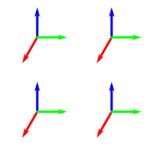
(b) $+1$

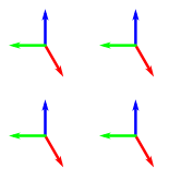
(c) $-1$

Figure 1: (Colors online) The arrows in panel a) $({\color[rgb]{0,0,1}\longrightarrow},{\color[rgb]{1,0,0}\longrightarrow},{\color[rgb]{0,1,0}\longrightarrow})$ correspond to $(\theta_{1},\theta_{2},\theta_{3})$. Panels (b) and (c) show examples of phase configurations for the two $\mathbb{Z}_{2}$ symmetry classes of the ground states, shown on a $2\times 2$ lattice of selected points of a planar slice of the system. Here $g_{12}>g_{23}>g_{13}>0$. The spatial contribution to the energy is minimized by making the spatial gradient zero (hence breaking the global $\mathrm{U}(1)$ symmetry). Then there are two classes of phase configurations, one with chirality +1 and one with chirality -1, minimizing the energy associated with the interband interaction. The chirality is defined as $+1$ if the phases (modulo $2\uppi$) are cyclically ordered $\theta_{1}<\theta_{2}<\theta_{3}$, and $-1$ if not.

In Ref. Bojesen et al., 2013 it was shown that in a multiband $\mathrm{U}(1)\times\mathbb{Z}_{2}$ superconductor only the $\mathrm{U}(1)$ sector, and not the $\mathbb{Z}_{2}$ sector, couples to a gauge field. Hence, if we induce vortices in such a superconductor by an external field, the behavior of the $\mathbb{Z}_{2}$ sector is expected to be largely unaffected. Thus, by applying an external field to a $\mathrm{U}(1)\times\mathbb{Z}_{2}$ superconductor, one should be able to control the $\mathrm{U}(1)$ sector independently of the $\mathbb{Z}_{2}$ sector, an effect which should be experimentally detectable.

Of special interest is the study of the $\mathrm{U}(1)$ symmetric, but $\mathbb{Z}_{2}$ broken metallic phase predicted to be present in the multiband superconductors for a range of parameters.Bojesen et al. (2014, 2013) We show that by tuning an external magnetic field, it is possible to extend the region of the $\mathbb{Z}_{2}$ broken metallic phase in the phase diagram.

II Models

In this work, we consider two versions of a 3D minimal $n$-component model in the London limit of the Ginzburg-Landau model of a multiband superconductor, displaying $\mathrm{U}(1)\times\mathbb{Z}_{2}$ symmetry. We focus on the simplest non-trivial case of three components. Both versions of the model are described in greater detail in Ref. Bojesen et al., 2014, see also reference therein. In particular, it has been shown Weston and Babaev (2013) that the inclusion of more than three superconducting bands crossing the Fermi surface will, apart from states with measure zero in parameter space, yield the same physics as in the three-band case. We include a non-fluctuating $\mathrm{U}(1)$ gauge field with a tunable value in the description, which in turn will lead to induced vortices. Neglecting the fluctuations in the amplitudes of the order-parameter components and the $\mathrm{U}(1)$ gauge-field is consistent with the fact that the pnictide superconductors are in the extreme type-II regime. V. and Kivelson (1995); Tes˘anović (1999); Nguyen and Sudbø (1999) The use of the London limit therefore rests on solid ground in this case.

II.1 Full model

The model on the $L^{3}$ lattice (with periodic boundary conditions) is given by

$$H=-\sum_{\langle i,j\rangle,\alpha}a_{\alpha}\cos(\theta_{\alpha,i}-\theta_{\alpha,j}-A_{ij})\\ +\sum_{i,\alpha^{\prime}>\alpha}g_{\alpha\alpha^{\prime}}\cos(\theta_{\alpha,i}-\theta_{\alpha^{\prime},i}),$$ (1)

where the gauge field is chosen to be

$$\bm{A}(\bm{r})=(2\uppi yf,0,0).$$ (2)

$i$ and $j$ are lattice site indices and $\langle i,j\rangle$ denote nearest neighbor sites. $\alpha,\alpha^{\prime}\in\set{1,2,\ldots,n}$ are component labels. $f$ is the vortex filling fraction, which is a direct measure of the rotation of the system. Moreover, $a,g>0$ are parameters determining the condensate density and intercomponent Josephson interaction, respectively. For convenience $a_{1}$ is set to $a_{1}=1$. Note that we have rescaled the gauge field $\bm{A}$ with the electric charge $e$, $\bm{A}\leftarrow e\bm{A}$.

II.2 Reduced ($K_{1}K_{2}$) model

Previous works Bojesen et al. (2014) have shown that the interband fluctuations of the phases of the “full” model, Eq. 1, are not of qualitative importance when mapping out the phase diagram. These fluctuations may be suppressed by letting $g_{\alpha\alpha^{\prime}}\to\infty$ while keeping the ratios $g_{\alpha\alpha^{\prime}}/g_{\alpha^{\prime\prime}\alpha^{\prime\prime\prime}}$ finite, locking the phase “stars” to one of their two ground state configurations, see Figs. 1b and 1c. The advantage of doing so is twofold. First, the $\mathrm{U}(1)\times\mathbb{Z}_{2}$ structure of the system is brought out clearly. Secondly, the computational cost of simulations is significantly reduced, meaning that larger systems and better statistics are obtainable.

The Hamiltonian may now be written asBojesen et al. (2014)

$$H=-\sum_{\langle i,j\rangle}(1+K_{1}\sigma_{i}\sigma_{j})\cos(\theta_{i}-\theta_{j}-A_{ij})\\ -\sum_{\langle i,j\rangle}K_{2}(\sigma_{i}-\sigma_{j})\sin(\theta_{i}-\theta_{j}-A_{ij})$$ (3)

Here $\sigma_{j}$ is a statistically fluctuating Ising-variable on each lattice site, denoting the chirality of the phase-star, while $\theta_{j}$ is a statistically varying $\mathrm{U}(1)$-variable denoting the overall orientation of the phase-star, see Fig. 2 as well as Figs. 1b and 1c. $K_{1}$ and $K_{2}$ are parameters given by

$$K_{1}\equiv \frac{\sum_{\alpha>1}a_{\alpha}\bigl{[}1-\cos(2\phi_{\alpha})\bigr{]}}{2+\sum_{\alpha>1}a_{\alpha}\bigl{[}1+\cos(2\phi_{\alpha})\bigr{]}}$$ (4)

$$K_{2}\equiv \frac{\sum_{\alpha>1}a_{\alpha}\sin(2\phi_{\alpha})}{2+\sum_{\alpha>1}a_{\alpha}\bigl{[}1+\cos(2\phi_{\alpha})\bigr{]}},$$ (5)

where $\phi_{\alpha}$ is the phase difference between the the first and the $\alpha$’th component in the ground state phase star, as illustrated in Fig. 2.

Figure 2: (Colors online) One of the two $\mathbb{Z}_{2}$ phase configurations in the $g_{\alpha\alpha^{\prime}}\to\infty$ limit when $n=3$. $\phi_{\alpha}$ is the phase difference between the first and the $\alpha$’th component, a constant.

It can be shown that $K_{1}$ and $K_{2}$ are restricted to the ellipsis given by

$$\left[\frac{2}{n-1}K_{1}-1\right]^{2}+\left[\frac{2\sqrt{n}}{n-1}K_{2}\right]^{2}\leq 1.$$ (6)

An equivalent formulation to Eq. 3 reads (see Appendix A)

$$H=-\sum_{\langle i,j\rangle}(1+J\sigma_{i}\sigma_{j})\cos(\theta_{i}-\theta_{j}-A_{ij}-\alpha(\sigma_{i},\sigma_{j}))$$ (7)

where

$$\alpha(\sigma_{i},\sigma_{j})\equiv\begin{cases}0&\sigma_{i}=\sigma_{j}\\ \pm\arctan\left[\frac{2K_{2}}{1-K_{1}}\right]&\sigma_{i}=-\sigma_{j}=\pm 1\end{cases}$$ (8)

and

$$J=\frac{W}{1+\sqrt{1-W^{2}}}\in[0,K_{1}],$$ (9)

where

$$W\equiv\frac{2(K_{1}-{K_{2}}^{2})}{1+{K_{1}}^{2}+2{K_{2}}^{2}}.$$ (10)

Equation 7 reveals an interesting feature of the model. $K_{2}\neq 0$, i.e. when the system features a deviation from a symmetric ground state phase star (i.e. $\phi_{12}\neq\phi_{13}\neq\phi_{23}$ in the $n=3$ case), leads to the addition of a fluctuating quantity coupling minimally to the phase-difference on a link, $\theta_{i}-\theta_{j}$. It formally has the appearance of a fluctuating discrete “gauge field”, $\alpha$, in a Ising-XY model. It should be kept in mind, however, that $\alpha(\sigma_{i},\sigma_{j})$ is only a “semi-independent” degree of freedom since it couples to the prefactor through the $J\sigma_{i}\sigma_{j}$ term.

III Observables

In the full model, as well as in the reduced one, the $\mathbb{Z}_{2}$ sector is monitored by the (global) “magnetization” defined as

$$m\equiv N^{-1}\sum_{i}\sigma_{i}$$ (11)

We use the Binder cumulant,Binder (1981); Sandvik (2010)

$$U_{2}\equiv\frac{1}{2}\left(3-\frac{\left\langle m^{4}\right\rangle}{\left\langle m^{2}\right\rangle^{2}}\right),$$ (12)

to detect phase transitions. The Binder cumulant displays a non-analytical jump at the phase transition in the thermodynamical limit, and has the useful property of being only mildly affected by finite size effects.

For the reduced model, we use the helicity modulus along the $z$-axis, the direction of the external field, to probe the structural order of the vortex system. Furthermore, to make sure that there is no pinning of the vortices to the underlying numerical lattice, we monitor the helicity modulus in the $x$ and $y$ directions as well. These should be zero for all temperatures of interest if such numerical artifacts are to be avoided.

In the full model, the helicity modulus is no longer well defined if one wants to consider the formation of a vortex lattice in each of the individual components. We choose therefore instead to use the value of the planar structure function of the vortices at the first Bragg peak to monitor the vortex lattice as the temperature is varied. In the liquid phase this will be a small number (approaching zero in the thermodynamical limit), while in the ordered phase this number will be finite. The structure function for a given momentum $\bm{k}_{\perp}$ in the plane perpendicular to the direction of the external field, the $xy$ plane, is given by

$$S^{\alpha}(\bm{k}_{\perp})=\frac{1}{(fL^{3})^{2}}\biggl{\langle}\Bigl{|}\sum_{\bm{r}}n_{z}^{\alpha}(\bm{r})\,\mathrm{e}^{\mathrm{i}\bm{k}_{\perp}\cdot\bm{r}_{\perp}}\Bigr{|}^{2}\biggr{\rangle}$$ (13)

$\bm{r}_{\perp}$ is the projection of the position vector $\bm{r}$ onto the $xy$ plane. $\bm{n}^{\alpha}(\bm{r})$ is the vorticity vector (which can be $0,\pm 1$ in each spatial component) of component $\alpha$ of the field in point $\bm{r}$,

$$\bm{n}^{\alpha}(\bm{r})=\frac{1}{2\uppi}[\nabla\times(\nabla\theta_{\alpha}-e\bm{A})]$$ (14)

We also monitor the specific heat,

$$c\equiv N^{-1}C=N^{-1}\beta^{2}\big{\langle}(H-\left\langle H\right\rangle)^{2}\big{\rangle}.$$ (15)

IV Simulations and Results

Due to the frustration effects inherent in the models, there appears to be no efficient nonlocal (cluster) algorithm for simulating them. Hence, a local update Monte Carlo scheme, the “Fast Linear Algorithm” (FLA) of Ref. Loison et al., 2004, was used. It proved to be a significant improvement over the standard Metropolis-Hastings sampling, and appears to be the most efficient canonical algorithm available for the models investigated in this paper. However, for technical reasons the use of FLA meant that we were prevented from simulating the case $K_{1}=1$ of the reduced model, where the effect of the intraband frustration is strongest in a three component reduced model. Therefore, in the simulations, the parameter-value $K_{1}=0.99$ was chosen as a reasonable compromise between proximity to $K_{1}=1$ and numerical stability.

In order to take advantage of the computational resources available, grid parallellization was implemented. Ferrenberg-Swendsen multi-histogram reweighting Ferrenberg and Swendsen (1989) was used to improve our numerical data. Pseudorandom numbers were generated by the Mersenne–Twister algorithm Matsumoto and Nishimura (1998).

The reduced model is significantly less computational demanding than the full model, and most of the simulations were performed on the former. To demonstrate the equivalence of the two models, we first show that the full model gives equivalent results to the reduced model for a representative choice of parameters. (See also Ref. Bojesen et al., 2014.)

Moreover, we establish the main point conjectured earlier, namely that an external field separates the $\mathbb{Z}_{2}$ transition and the $\mathrm{U}(1)$ lattice melting, with separation increasing with field strength since the external gauge-field couples to the $\mathrm{U}(1)$-sector, but not the $\mathbb{Z}_{2}$- sector. Thus, as magnetic field is increased, we observe a reversal of the order of the $\mathrm{U}(1)$ and $\mathbb{Z}_{2}$ transitions as a function of temperature.

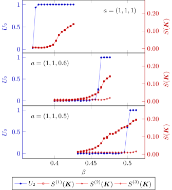
Figure 3: Simulation results for the full model with $a$ as indicated, and $g=(5,5,5)$, $f=\tfrac{1}{32}$, and $L=64$. The $\mathbb{Z}_{2}$ sector is monitored by the Binder cumulant for the $\mathbb{Z}_{2}$ magnetization, $U_{2}$ (blue). The vortex lattice ordering (in each component) is monitored by the value of the structure function at the first Bragg peak, $S(\bm{K})$ (red). Note how the order of the phase transitions changes as the anisotropy of the system $a_{3}/a_{1,2}$ is varied. In the top panel, the system features a normal metallic state (vortex liquid), with broken $\mathbb{Z}_{2}$ symmetry being restored at $\beta\approx 0.37$. In the bottom panel, the $\mathbb{Z}_{2}$ symmetry is restored inside the superconducting (vortex lattice) phase. In the middle panel, the transitions occur roughly simultaneously. (Colors online.)

Figure 3 shows simulation results from the full model, Eq. 1, for various different choices $a_{3}$ of the model, with fixed $a_{1}=a_{2}=1$. This variation effectively leads to a variation in the angles $\phi_{\alpha}$ describing the relative orientations of the various phases of the components of the order parameter in the ground state, and hence to a variation in the energy of the $\mathbb{Z}_{2}$ domain walls of the system. This in turn will lead to a variation in the critical temperature of the $\mathbb{Z}_{2}$ phase transition responsible for restoring time-reversal symmetry. The rotation of the system is fixed at a filling fraction $f=\tfrac{1}{32}$.

The top panel of Fig. 3 corresponds to the fully symmetric case where all $a_{\alpha}$ and $g_{\alpha,\alpha^{\prime}}$ are equal in Eq. 1, in turn corresponding to the case $K_{2}=0$ in Eq. 5. Reducing $a_{3}$ in the following panels shifts the $\mathbb{Z}_{2}$ phase transition downwards in temperature as the domain wall energy decreases. The transition temperature in the $\mathrm{U}(1)$-sector, in this case the vortex-lattice melting transition, is little affected by the reduction in $a_{3}$, since the vortex-lattice melting temperature is largely determined from the phase-stiffness of the overall phase-star, and not the relative-fluctuations of the internal phases of the multi-component order parameter. The former stiffness is dominated by the largest phase-stiffnesses of the individual phases, see for instance Eq. (2) of Ref. Bojesen et al., 2013. Thus, the $\mathbb{Z}_{2}$ transition temperature is eventually lowered through the $\mathrm{U}(1)$ transition temperature. This reversal of the phase transition of the $\mathbb{Z}_{2}$ and $\mathrm{U}(1)$ sectors means that the system transitions from one featuring a superconducting state with broken time-reversal symmetry and a time-reversal symmetric metal, to one with a time-reversal symmetric superconducting state and a metallic state with a spontaneously broken time-reversal symmetry. Below, we return to the experimental probes of the $\mathbb{Z}_{2}$ phase transition inside the superconducting or metallic states.

The results of Fig. 3 should be compared with the results for the reduced model, Fig. 4. For $K_{2}=0$, corresponding to the results shown in the upper panel of Fig. 3, the same result is found for smaller $K_{2}$ values, i.e the $\mathbb{Z}_{2}$ transition is found at higher temperature than the $\mathrm{U}(1)$ due to the relatively large energy of the $\mathbb{Z}_{2}$ domain-walls. As $K_{2}$ increases, the relative energy associated with a $\mathbb{Z}_{2}$ domain wall decreases, eventually resulting in a reversal of the order of the $\mathbb{Z}_{2}$ and $\mathrm{U}(1)$ transitions. These effects are thus essentially the same in the full and reduced models.

We next consider the effect of varying the rotation $f$ at otherwise fixed parameters. For this, we limit the discussion to the reduced model, Eq. 3. Figure 5 show how, as conjectured, the separation of the $\mathbb{Z}_{2}$ and $\mathrm{U}(1)$ transitions increase with an increasing external field strength. To work with a manageable parameter space, we limit the study to $K_{2}=0$ since this suffices to illustrate our main point, namely the separation of two otherwise simultaneous zero-field phase transitions when the field strength is increased. For the special case $f=0$, the $\mathbb{Z}_{2}$ and $\mathrm{U}(1)$ transitions occur simultaneously via a preemptive first-order mechanism, and there is never a chiral metallic state in the absence of a fluctuating gauge field Bojesen et al. (2014). As the field strength is increased, the transitions separate, with the $\mathrm{U}(1)$ transition being strongly suppressed to lower temperature while the $\mathbb{Z}_{2}$ transition remains only weakly affected. This follows from the fact that it is only the $\mathrm{U}(1)$-sector of the theory which couples to the (non-fluctuating) gauge field, while the $\mathbb{Z}_{2}$-sector does not. Hence, upon increasing the (non-fluctuating) gauge-field and hence the filling fraction of the system, the vortex-lattice melting transition of the $\mathrm{U}(1)$-sector is suppressed in the usual manner, while the $\mathbb{Z}_{2}$-sector is largely unaffected. A reversal of the order of the phase-transitions as the temperature is varied, is thus possible. An increase of the magnetic field beyond the vortex-lattice melting transition brings about a resistive state with spontaneously broken $\mathbb{Z}_{2}$-symmetry, a chiral metallic state.

Note that the temperature dependence of the structure function in Fig. 3 and the helicity moduli in Figs. 4 and 5 typically is not of the form one expects in a first-order vortex lattice transition, with a jump in the helicity modulus at the melting transition, and which has been found in the single-component case Hu et al. (1997); Nguyen and Sudbø (1999). This point requires further investigation, but is beyond the scope of the present paper, where the main point is not to investigate the details of the melting transition, but to demonstrate that a magnetic field may be utilized to clearly bring out the unusual metallic state with a spontaneously broken time-reversal symmetry.

Figures 6 and 7 show the specific heat corresponding to the results of Figs. 4 and 5. The main point to be made in connection with Figs. 6 and 7 is that the Ising-type anomaly in the vortex-liquid phase, associated with restoring the spontaneously broken time-reversal symmetry, is considerably more pronounced than the small anomaly associated with the vortex lattice melting. These two phase-transitions essentially involve the same degrees of freedom, ultimately connected to the phases $\theta_{\alpha,j}$ of the superconducting order-parameter components. Hence, to the extent that the specific heat anomaly associated with the vortex-lattice melting is observable, the Ising-anomaly inside the vortex-liquid phase, associated with restoring the broken $\mathbb{Z}_{2}$-symmetry, should be readily observable in specific-heat measurements on Fe-pnictides. Moreover, an equally prominent $\mathbb{Z}_{2}$-anomaly in the specific heat should be observable inside the vortex-lattice state, for small enough magnetic fields.

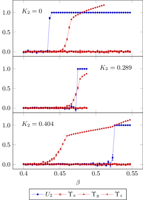
Figure 4: Simulation results for the reduced model with $K_{1}=0.99$, $f=\tfrac{1}{32}$, $L=128$ and $K_{2}=0,$0.058$,$0.173$,$0.289$,$0.404$$. The choice of the parameter $K_{1}$ is explained in the text. The $\mathbb{Z}_{2}$ sector is monitored by the Binder cummulant for the $\mathbb{Z}_{2}$ magnetization, $U_{2}$ (blue). The vortex lattice ordering is monitored by the helicity modulus, $\Upsilon$, (red) in the various directions, where $z$ is parallel to the external field. (Colors online.)

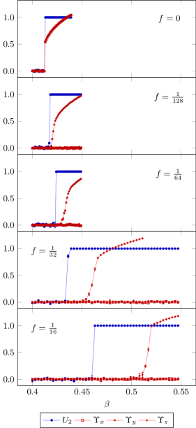
Figure 5: Simulation results for the reduced model with $K_{1}=0.99$, $K_{2}=0.0$, $L=128$ and $f=0,\tfrac{1}{128},\tfrac{1}{64},\tfrac{1}{32},\tfrac{1}{16}$. The $\mathbb{Z}_{2}$ sector is monitored by the Binder cumulant for the $\mathbb{Z}_{2}$ magnetization, $U_{2}$ (blue). The vortex lattice ordering is monitored by the helicity modulus, $\Upsilon$, (red) in the various directions, where $z$ is parallel to the external field. In zero external field ($f=0$) the system is isotropic. (Colors online.)

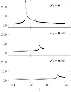
Figure 6: Specific heat capacity of the reduced model with $K_{1}=0.99$, $f=\tfrac{1}{32}$, $L=128$ and $K_{2}=0,$0.289$,$0.404$$. Associated with Fig. 4.

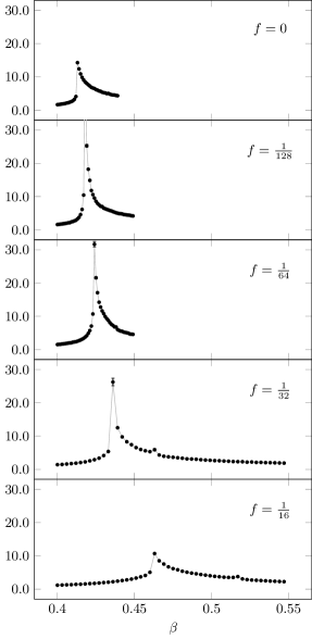
Figure 7: Specific heat of the reduced model with $K_{1}=0.99$, $K_{2}=0.0$, $L=128$ and $f=0,\tfrac{1}{128},\tfrac{1}{64},\tfrac{1}{32},\tfrac{1}{16}$. These results correspond to those shown in Fig. 5. Note that the $\mathbb{Z}_{2}$-anomaly is considerably more prominent than the sharp peak associated with the melting of the vortex lattice.

V Summary and conclusions

We have studied two models describing $\mathrm{U}(1)\times\mathbb{Z}_{2}$ multiband superconductors in the London limit, subject to an external field. We have focused on the three-component case. The external field induces vortices in the condensate, leading to an increased separation of, and indeed reversal of, the $\mathbb{Z}_{2}$ and $\mathrm{U}(1)$ phase transitions as the temperature is varied. This brings out clearly the domain of a metallic (vortex liquid state) with an additional spontaneously broken time-reversal symmetry on top of the explicitly broken time-reversal symmetry from the external field. The effect increases with increasing field. Inside the vortex-liquid phase there should be an anomaly in the specific heat, and this anomaly should be in the 3D Ising universality class. The same degrees of freedom are involved in disordering the vortex lattice as are involved in disordering the chirally ordered state. The numeric results show that both anomalies are observable, but the $\mathbb{Z}_{2}$-anomaly is considerably easier to see, see Figs. 6 and 7. Hence, we expect that this anomaly associated with restoring the $\mathbb{Z}_{2}$ chiral order to be readily observable in experiments. Moreover, the same should be the case for the $\mathbb{Z}_{2}$-anomaly in the specific heat inside the vortex-lattice for small enough magnetic fields. Finally, we note that the predictions of anomalies in the specific, obtained in the London-limit of the Ginzburg-Landau theory of a multi-band superconductor, should be robust to inclusion of amplitude fluctuations in the order-parameter components. Such fluctuations are non-critical, but will nonetheless tend to enhance the specific heat-anomalies, albeit analytically as a function of temperature.

T.A.B. thanks NTNU for financial support, and the Norwegian consortium for high-performance computing (NOTUR) for computer time. A.S. was supported by the Research Council of Norway, through Grants 205591/V20 and 216700/F20. AS thanks the Aspen Center for Physics (NSF Grant No 1066293) for hospitality during the initial stages of this work.

Appendix A Derivation of alternative reduced model

We derive Eq. 7 from Eq. 3.

The identity

$$A\cos x+B\sin x=\sqrt{A^{2}+B^{2}}\cos\left[x-\arctan\left(\tfrac{B}{A}\right)\right],$$ (16)

together with $\sigma_{i}^{2}=1$, implies that the contribution from a lattice link to the Hamiltonian, Eq. 3, can be written on the form

$$H_{ij}={} -(1+K_{1}\sigma_{i}\sigma_{j})\cos(\theta_{i}-\theta_{j}-A_{ij})$$

$$-K_{2}(\sigma_{i}-\sigma_{j})\sin(\theta_{i}-\theta_{j}-A_{ij})$$

$$={} -(p+q\sigma_{i}\sigma_{j})\cos(\theta_{i}-\theta_{j}-A_{ij}-\alpha(\sigma_{i},\sigma_{j})).$$ (17)

$p$,$q$, and $\alpha$ are functions of $K_{1}$ and $K_{2}$, to be determined.

Comparing with Eq. 16, it is seen that $\alpha$ is given by

$$\alpha =\arctan\left[\frac{K_{2}(\sigma_{i}-\sigma_{j})}{1+K_{1}\sigma_{i}\sigma_{j}}\right]$$

$$=\begin{cases}0&\sigma_{i}=\sigma_{j}\\ \pm\arctan\left[\frac{2K_{2}}{1-K_{1}}\right]&\sigma_{i}=-\sigma_{j}=\pm 1\end{cases}$$ (18)

Similarly, $p$ and $q$ are determined by

$$\sqrt{(1+K_{1}\sigma_{i}\sigma_{j})^{2}+{K_{2}}^{2}(\sigma_{i}+\sigma_{j})^{2}}=p+q\sigma_{i}\sigma_{j},$$ (19)

or, by squaring both sides,

$$1+{K_{1}}^{2}+2{K_{2}}^{2}+2(K_{1}-{K_{2}}^{2})\sigma_{i}\sigma_{j}=p^{2}+q^{2}+2pq\sigma_{i}\sigma_{j}.$$ (20)

Comparing the two sides, we see that

$$p^{2}+q^{2} =1+{K_{1}}^{2}+2{K_{2}}^{2}\equiv U,$$ (21)

$$pq =K_{1}-{K_{2}}^{2}\equiv V.$$ (22)

Combining these two equations, yields the quadratic equation in $p^{2}$

$$p^{4}-Up^{2}+V^{2}=0,$$ (23)

with solutions

$$p=\pm\sqrt{\tfrac{1}{2}\left(U\pm\sqrt{U^{2}-4V^{2}}\right)}.$$ (24)

When $K_{2}=0$, $p+q\sigma_{i}\sigma_{j}$ should reduce to $1+K_{1}\sigma_{i}\sigma_{j}$. Hence, the relevant solution is

$$p =\sqrt{\tfrac{1}{2}\left(U+\sqrt{U^{2}-4V^{2}}\right)},$$ (25)

$$q =\frac{V}{p}.$$ (26)

Rescaling the Hamiltonian by $1/p$ simplifies Eq. 17 to

$$H_{ij}=-\left(1+J\sigma_{i}\sigma_{j}\right)\cos(\theta_{i}-\theta_{j}-A_{ij}-\alpha(\sigma_{i},\sigma_{j})),$$ (27)

where $J$ is given by Eqs. 9 and 10. Thus, since $H=\sum_{\langle i,j\rangle}H_{ij}$, we have derived Eq. 7.

For $n\geq 3$, we have $W\in[0,2K_{1}/(1+{K_{1}}^{2})<1]$, since $K_{1}\in[0,n-1]$ and $K_{1}\geq{K_{2}}^{2}$. $J(W)$ increases monotonically with $W$ for $W\in[0,1)$, so

$$J\in[0,K_{1}].$$ (28)

References

- Seyfarth et al. (2005) G. Seyfarth, J. Brison, M.-A. Measson, J. Floquet, K. Izawa, Y. Matsuda, H. Sugawara, and H. Sato, Phys. Rev. Lett 95, 107004 (2005).
- Kamihara et al. (2008) Y. Kamihara, T. Watanabe, M. Hirano, and H. Hosono, J. Am. Chem. Soc. 130, 3296 (2008).
- Prakash et al. (2008) J. Prakash, S. J. Singh, S. L. Samal, S. Patnaik, and A. K. Ganguli, EPL (Europhysics Letters) 84, 57003 (2008).
- Lu et al. (2009) D. Lu, M. Yi, S.-K. Mo, J. Analytis, J.-H. Chu, A. Erickson, D. Singh, Z. Hussain, T. Geballe, I. Fisher, and Z.-X. Shen, Physica C: Superconductivity 469, 452 (2009), superconductivity in Iron-Pnictides.
- Liu et al. (2009) C. Liu, T. Kondo, A. Palczewski, G. Samolyuk, Y. Lee, M. Tillman, N. Ni, E. Mun, R. Gordon, A. Santander-Syro, S. Bud’ko, J. McChesney, E. Rotenberg, A. Fedorov, T. Valla, O. Copie, M. Tanatar, C. Martin, B. Harmon, P. Canfield, R. Prozorov, J. Schmalian, and A. Kaminski, Physica C: Superconductivity 469, 491 (2009), superconductivity in Iron-Pnictides.
- Kuroki and Aoki (2009) K. Kuroki and H. Aoki, Physica C: Superconductivity 469, 635 (2009), superconductivity in Iron-Pnictides.
- Subedi et al. (2008) A. Subedi, L. Zhang, D. J. Singh, and M. H. Du, Phys. Rev. B 78, 134514 (2008).
- Stanev and Tešanović (2010) V. Stanev and Z. Tešanović, Phys Rev B 81, 134522 (2010).
- Maiti and Chubukov (2013) S. Maiti and A. V. Chubukov, Phys. Rev. B 87, 144511 (2013), arXiv:1302.2964 [cond-mat.supr-con] .
- Weston and Babaev (2013) D. Weston and E. Babaev, Phys. Rev. B 88, 214507 (2013).
- Bojesen et al. (2014) T. A. Bojesen, E. Babaev, and A. Sudbø, Phys. Rev. B 89, 104509 (2014).
- Bojesen and Sudbø (2014) T. Bojesen and A. Sudbø, Phys Rev (submitted) (2014), arXiv:1407.0711 .
- Bojesen et al. (2013) T. A. Bojesen, E. Babaev, and A. Sudbø, Phys. Rev. B 88, 220511 (2013).
- Ng and Nagaosa (2009) T. K. Ng and N. Nagaosa, Europhys. Lett. 87, 17003 (2009).
- Stanev (2012) V. Stanev, Phys. Rev. B 85, 174520 (2012), arXiv:1108.2501 [cond-mat.supr-con] .
- Carlström et al. (2011) J. Carlström, J. Garaud, and E. Babaev, Phys. Rev. B 84, 134518 (2011).
- V. and Kivelson (1995) E. V. and S. Kivelson, Nature 374, 434 (1995).
- Tes˘anović (1999) Z. Tes˘anović, Phys. Rev. B 59, 6449 (1999).
- Nguyen and Sudbø (1999) A. K. Nguyen and A. Sudbø, Phys. Rev. B 60, 15307 (1999).
- Note (1) The reduced model is less computationally demanding than the full model for several reasons, the most important one being the reduction of degrees of freedom per lattice site.
- Binder (1981) K. Binder, Zeitschrift für Physik B Condensed Matter 43, 119 (1981).
- Sandvik (2010) A. W. Sandvik, in American Institute of Physics Conference Series, American Institute of Physics Conference Series, Vol. 1297, edited by A. Avella and F. Mancini (2010) pp. 135–338, arXiv:1101.3281 [cond-mat.str-el] .
- Loison et al. (2004) D. Loison, C. Qin, K. Schotte, and X. Jin, The European Physical Journal B - Condensed Matter and Complex Systems 41, 395 (2004).
- Ferrenberg and Swendsen (1989) A. M. Ferrenberg and R. H. Swendsen, Phys. Rev. Lett. 63, 1195 (1989).
- Matsumoto and Nishimura (1998) M. Matsumoto and T. Nishimura, ACM Trans. Model. Comput. Simul. 8, 3 (1998).
- Hu et al. (1997) X. Hu, S. Miyashita, and M. Tachiki, Phys. Rev. Lett. 79, 3498 (1997).