Comet C/2013 A1 (Siding Spring) as seen with the
Herschel Space Observatory

The thermal emission of comet C/2013 A1 (Siding Spring) was observed on March 31, 2013, at a heliocentric distance of 6.48 au using the PACS photometer camera of the Herschel Space Observatory. The comet was clearly active, showing a coma that could be traced to a distance of $\sim$10″, i.e. $\sim$50000 km. Analysis of the radial intensity profiles of the coma provided dust mass and dust production rate; the derived grain size distribution characteristics indicate an overabundance of large grains in the thermal emission. We estimate that activity started about 6 months before these observations, at a heliocentric distance of $\sim$8 au.

1 Introduction

Comet C/2013 A1 (Siding Spring) will approach Mars to 140 000 km on October 19, 2014 and may cause a notable fluence of large, high velocity particles, posing a threat on instruments working either on the planet’s surface or in Martian orbits. Several authors performed hazard analysis based on various datasets (Farnocchia et al., 2014; Kelley et al, 2014; Tricarico et al., 2014; Ye & Hui, 2014) and in most cases obtained a low fluence of dust particles at the critical places. In this letter we report on the Herschel/PACS observations of the comet, analyse the coma structure and construct simple models to estimate the dust production rate, grain size distribution and onset time of the comet’s activity. These far-infrared observations are particulary well suited to complement previous observations used for dust particle impact calculations, as they were obtained 1.5 years before the encounter. Particles visible at the time of these infrared observations have the chance to reach the surface or close orbits around Mars (Kelley et al, 2014), while large dust grains ejected later will likely miss the surface of the red planet.

2 Observations and data reduction

Thermal emission of C/2013 A1 was observed with the PACS photometer camera (Poglitsch et al., 2010) of the Herschel Space Observatory (Pilbratt et al., 2010) using the time awarded in a DDT proposal exclusively for C/2013 A1 (proposal ID: DDT_pmattiss_1, P.I.: P. Mattisson). The observations were performed in mini-scanmap mode and covered all three bands using the configurations detailed in Table 1. At the time of the observations the target was at a heliocentric distance of r = 6.479 au, at a distance of $\Delta$ = 6.871 au from Herschel, and at a phase angle of $\alpha$ = 7$\aas@@fstack{\circ}$98.

The data reduction is based on the pipeline developed for the ”TNOs are Cool!” Herschel Open Time Key Program (Müller et al., 2009; Kiss et al., 2014). The reduction of raw data was performed using an optimized version of the PACS bright point source pipeline script with the application of proper motion correction, i.e. the maps have been produced in the co-moving frame of the comet. While the movement of the target was significant, it did not move enough between two OBSIDs that the maps could be used as mutual backgrounds. Our images may therefore be affected by background features.

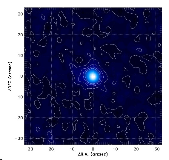
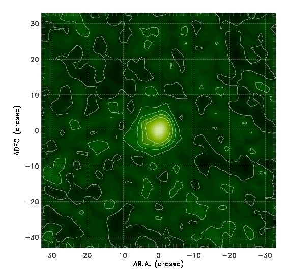
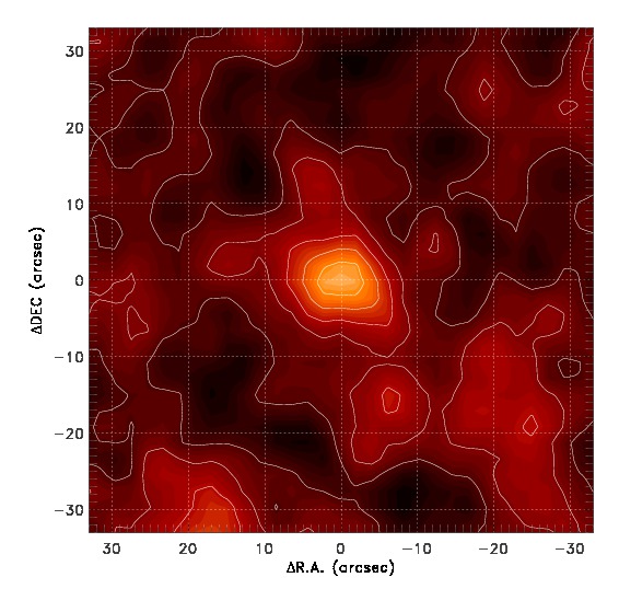
Figure 4: Co-moving frame, co-added images of C/2013 A1 in the Herschel/PACS 70 (top), 100 (middle) and 160 $\mu$m (bottom) bands.

Maps were created with both applying high-pass filtering (HPF) in combination with the photProject() task in HIPE, as well as using the standard JScanam pipeline. The HPF+photProject maps are better suited for point- and compact sources, since due to the high-pass filtering the large scale structure (extended emission) is not preserved. In contrast, JScanam maps keep the larger scale structures in the maps. The typical spatial scale on which extended emission is suppressed in HPF maps is $>$30″with our settings. The comparison of the HPF and JScanam maps show that they are practically identical in the central $\sim$30″area, and no additional extended emission could be identified at these distances on the JScanam maps. In addition, the HPF maps provided a significantly grater S/N ratio in the red band than the JScanam maps, therefore we used these HPF images for further analysis (Fig. 4).

Table 1: Summary of Herschel observations. The columns are: i) observation identifier (OBSID); ii) date and start time; iii) duration; v) filters configuration; vi) scan angle direction with respect to the detector array.

OBSID	Date	tobs	Filters	pscan
	& time	(s)	($\mu$m/$\mu$m)	(deg)
	2013-03-31
1342268974	18:10:51	1132	70/160	70
1342268975	18:30:46	1132	70/160	110
1342268976	18:50:41	1132	100/160	70
1342268977	19:10:36	1132	100/160	110

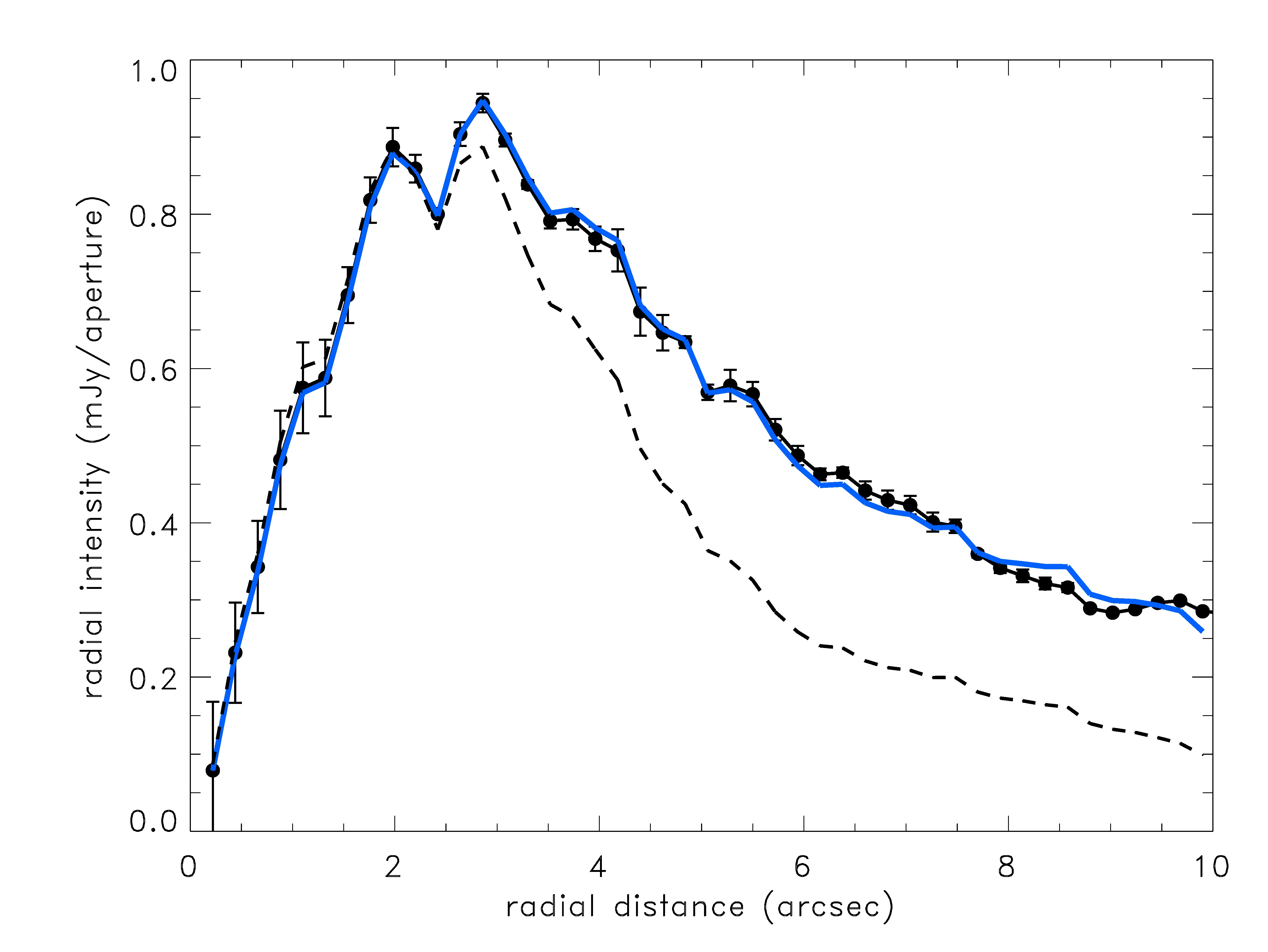
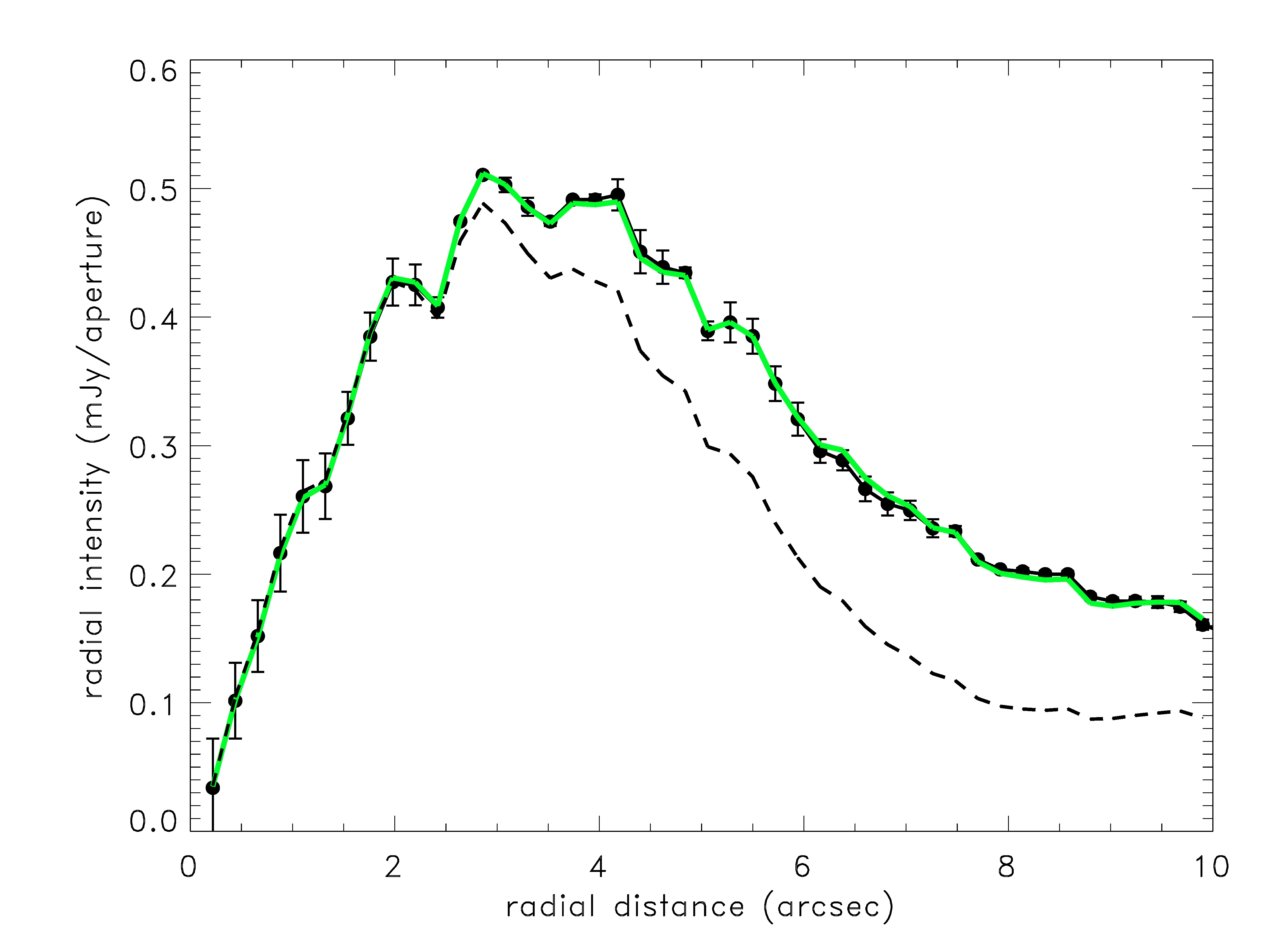
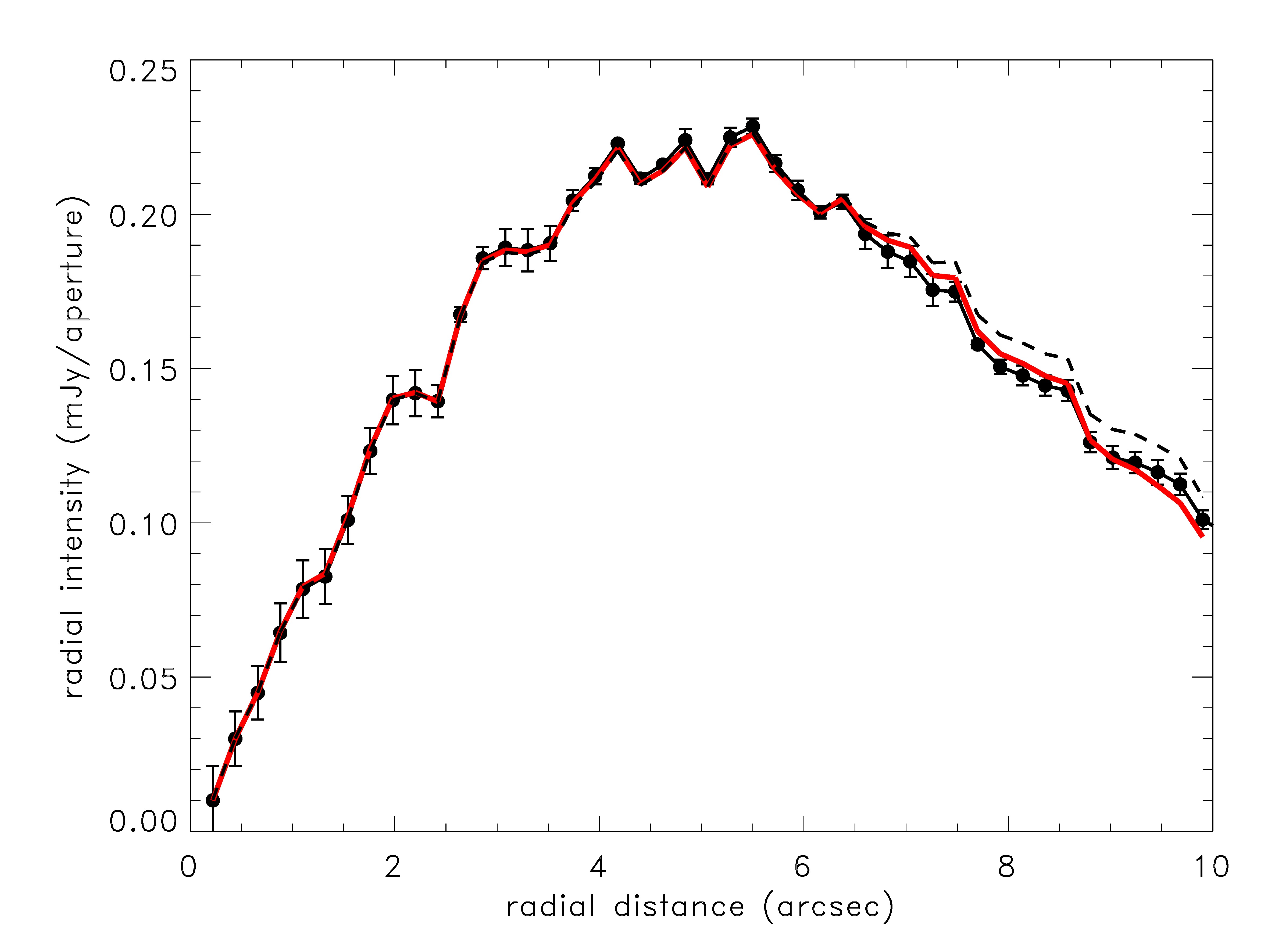
Figure 1: Radial intensity profiles in the three PACS band (70, 100 and 160 $\mu$, from left to right). The observed profiles are presented by black dots, while colour curves represent the best fit model profiles according to Eq. 1 (see Table 2). The corresponding radial intensity profiles of the respective PACS PSFs are shown as dashed curves.

3 Intensity profile

The PSF width for PACS at 70, 100 and 160 $\mu$m is 5.7, 7.5 and 11.7″, respectively. We detect a clear broadening of the comet PSF out to 10″ ($\sim$50000 km) at 70 and 100 $\mu$m, allowing us to analyse the coma structure at these wavelengths. At 160 $\mu$m the coma structure is hardly resolvable due to the wide PSF and the impact of the sky background (Fig 1). With the aim of trying to separate the nucleus and the coma, we first fitted the radially averaged intensity profiles in all PACS band with a two component model. One component corresponds to the unresolved nucleus, assuming a Dirac-delta at the intensity peak, while the another component describes the coma, with a radially decreasing surface brightness, characterized by the scale length $r_{0}$ and the exponent $\gamma$:

$$F=k_{nucl}\delta(0)+{{k_{coma}}\bigg{(}1+\bigg{(}{r\over{r_{0}}}\bigg{)}^{\gamma}}\bigg{)}^{-1}$$ (1)

With these parameters we construct a 2D image that is convolved with the respective PSF of the fiducial calibration star $\gamma$ Dra to obtain a synthetic image and a corresponding radial intensity that is compared with the observed radial intensity profile. The best fit parameters are derived using a Levenberg-Marquardt fitter and are presented in Table 2. The best fit coma profiles provides a nucleus contribution of 12.8, 8.2 and 7.5 mJy at 70, 100 and 160 $\mu$m, respectively. In the red (160 $\mu$m) band this $k_{n}$ = 7.5 mJy flux covers basically the total thermal emission of the comet (see Table 2), mainly due to the wide PSF. If these fluxes are considered as a flux originated from a solid nucleus, the size of the body can be estimated by thermal model calculations (Müller & Lagerros, 1998, 2002) and results in a nucleus radius of r_n $\approx$ 11 km, with a geometric albedo of p_V = 5%. Higher spatial resolution measurements obtained later, e.g. the Hubble Space Telescope measurements (Hubble Space Telescope, Li et al., 2014, in prep.) provided a nucleus size of r_n $<$1 km indicating that the thermal emission contribution we observe is probably not originated from a solid body, but from a spatially unresolved, compact dust coma, likely inside the contact surface with the solar wind, as was observed in the case of 29P/Schwassmann-–Wachmann with Herschel/PACS (Bockelee-Morvan et al., 2010). This is also supported by the compact, unresolved coma at 160 $\mu$m.

We repeated the coma radial intensity profile fit without allowing any flux contribution from the nucleus or compact dust coma($k_{n}$ $\equiv$ 0). As the red (160 $\mu$m) profile is very close to the red point source PSF (see Fig. 1) we did not repeat this fit for this band. In the blue (70 $\mu$m) and green (100 $\mu$m) bands the radial intensity profiles can be fitted almost equally well as in the $k_{n}$ $\neq$ 0 case (see Table 2 and Fig. 1). The intensity decreases with the radial distance in both bands with $\gamma$ $\approx$ –2, slightly slower in the blue, indicating a relative excess of higher temperature / smaller particles at higher radial distances. The total fluxes derived from these fits are F₇₀ = 41$\pm$2 mJy and F₁₀₀ = 26 $\pm$2 mJy in the blue and green bands, respectively. When we calculate the ratio of the blue and green intensity profiles (with 70$\mu$m intensity profiles convolved to the 100 $\mu$m resolution) in the inner parts of the coma ($<$3″) show a constant ratio that corresponds to the characteristic temperature of large grains at this heliocentric distance, T $\approx$ 110 K. At larger radial distances ($>$5″ of the observed radial intensity profile), however, the flux ratios and hence the characteristic temperatures increase, indicating a relatively stronger presence of smaller grains in the outer regions.

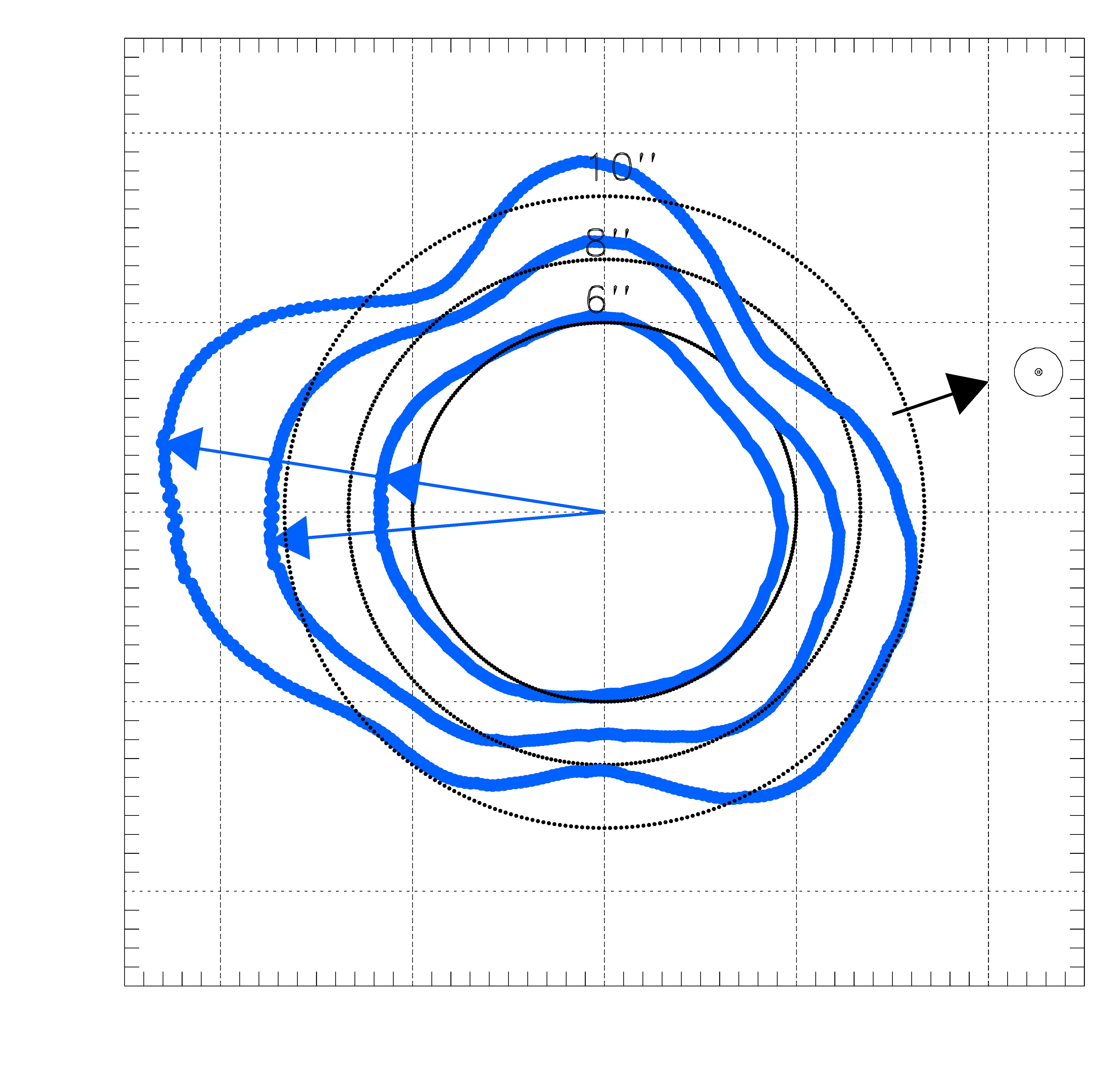
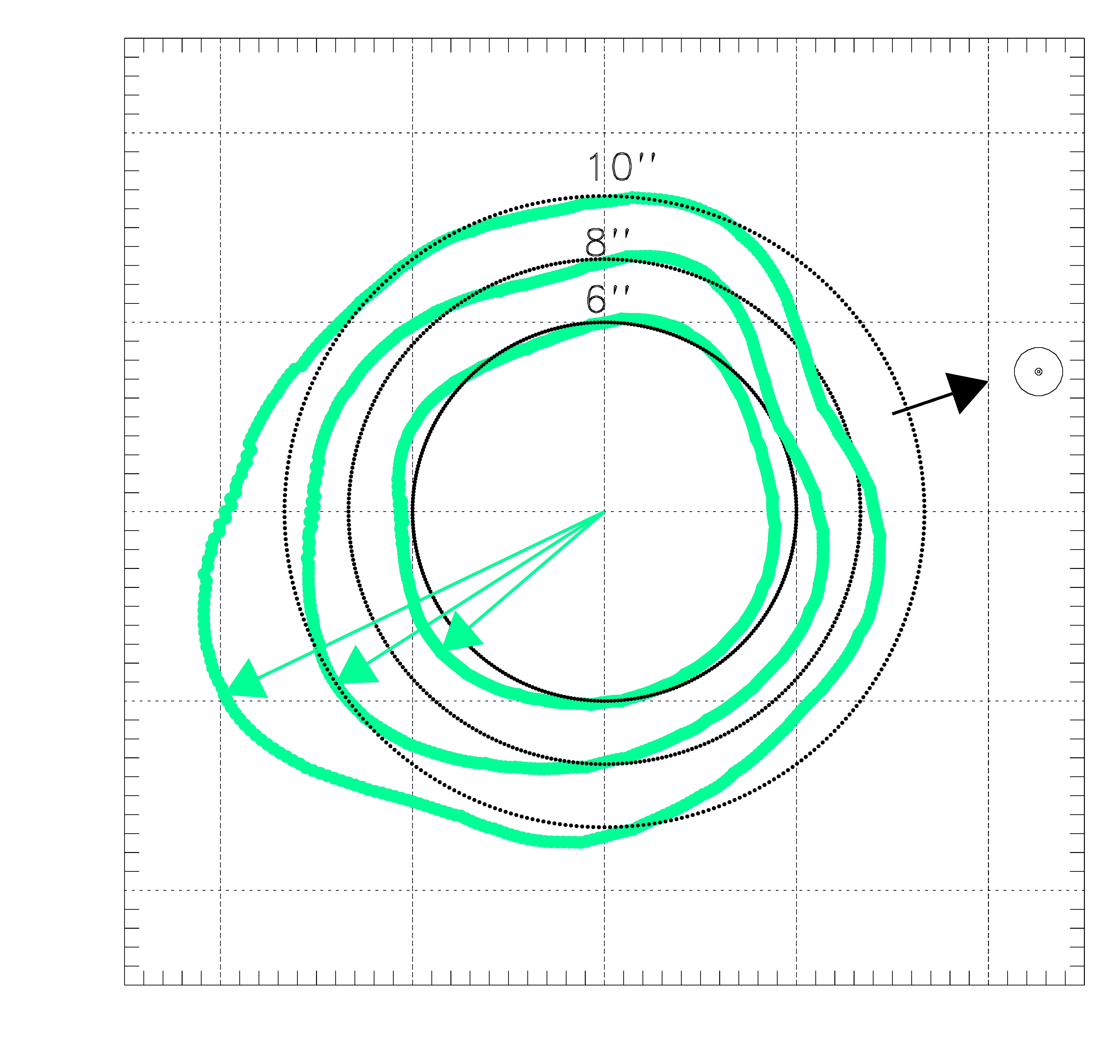
Figure 2: Dependence of integrated intensity on the position angle within 6″, 8″and 10″from the intensity peak for the blue (left panel) and green (right panel) maps. The contours show the intensity integrated in 30°  segments w.r.t. the average value. The circles correspond to the mean intensity at that specific radial distances, contours inside the circle indicate intensity below the average while coutours outside the circle indicate an excess. The coloured arrows show the the direction of the intensity maxima. The black arrow indicate the position angle of the Sun.

Table 2: Intensity profile fit results using Eq. 1. The intensity profiles were fitted both with and without including the contribution of a ”nucleus”

. PACS $k_{n}$ $k_{c}$ $\gamma$ $r_{0}$ band (mJy) (mJy/beam) (arcsec) with nucleus blue 12.8$\pm$0.7 0.13$\pm$0.02 1.89$\pm$0.04 2.51$\pm$0.14 green 8.2$\pm$0.8 0.12$\pm$0.03 2.15$\pm$0.05 2.54$\pm$0.16 red 7.5$\pm$1.2 – – – without nucleus blue – 8.72$\pm$0.05 1.83$\pm$0.23 0.23$\pm$0.04 green – 2.72$\pm$0.05 2.12$\pm$0.27 0.60$\pm$0.06

On the 70 and 100 $\mu$m images a slight elongation of the coma is observed. On these images we derive the position angle of this feature using the intensity integrated in a 30° cone out to a specific radial distance from the intensity peak (see Fig. 2). In the blue case the elongation contours are mostly affected by the strong tripod structure of the PACS 70 $\mu$m PSF, overriding any other possible structure. In the green band, however, the tripod structure is less pronounced and in this band we obtained PA = $-139$°, $-147$° and $-154$° at the radial distances of 6″, 8″and 10″. The position angle of the Sun was $\sim$19° at the time of the PACS observations.

4 Simple dust production rate estimate

From the observed thermal emission of the particles we can estimate the dust production rate in an $Af\rho$ manner (A’Hearn et al., 1984). We calculate the $Af\rho$ parameter from the 70 $\mu$m dust emission, as this emission is the least affected by the background. The thermal emission can be estimated as

$$F^{\nu}_{therm}={{1-\overline{A}}\over{A(\alpha)}}\pi B_{\nu}(T){{(Af\rho)}\over{\Delta^{2}}}\rho$$ (2)

where $\rho$ is the radial distance from the nucleus, $\overline{A}$ is the mean bolometric Bond albedo of the dust, A($\alpha$) is the phase angle dependent Bond albedo, $B_{\nu}(T)$ is the Planck function and we use the same parametrization as in Mommert et al. (2014). The dust temperature at this heliocentric distance is estimated to be 108-116 K for large ($>$10 $\mu$m) dust particles, with a slight dependence on the particles type. We adopt T = 110 K dust temperature and $\rho$ = 50 000 km radial distance that corresponds to 10″ apparent radial extension, resulting in a value of $Af\rho$ = 185$\pm$25 cm. When this value is compared with the $Af\rho$ values obtained from NEOWISE measurements at smaller heliocentric distances we found that the increase of the activity was faster between 4 and 6.5 au than would have been inferred from the (Stevenson et al., 2014) data alone. From this $Af\rho$ value we estimate the dust production rate:

$$Q_{dust}=(Af\rho){2\over{3}}{{{\rho_{d}}a{v_{d}}}\over{A_{p}}}$$ (3)

where $\rho_{d}$ is the dust density, $a$ the dust grain radius, $v_{d}$ the escape velocity, and $A_{p}$ the geometric albedo of the dust particles, assuming a fixed grain size. We adopt a = 15 $\mu$m, $\rho_{d}$ = 1 g cm^-3 and A_p = 0.15 (Kelley & Wooden, 2009). For this particle size the dust velocity is estimated as

$$v_{d}=v_{ref}\Big{(}{{a}\over{1\,mm}}\Big{)}^{-0.5}\Big{(}{{r_{h}}\over{5\,au}}\Big{)}^{-1}$$ (4)

Using v_ref = 1.9 m s^-1 (Kelley et al, 2014) this results in v_d = 12 m s^-1 for 15 $\mu$m-sized grains and Q_dust = 1.5$\pm$0.5 kg s^-1. We can compare these values with the NEOWISE $Af\rho$-based estimates of Q_dust = 11$\pm$4 and 45$\pm$15 kg s^-1 at 3.8 and 1.9 au heliocentric distances, respectively (Stevenson et al., 2014). These three Q_dust estimates agree relatively well with a power-law distance scaling of ($r_{h}$/$r_{0}$)${}^{q_{Q}}$, with an exponent of q_Q $\approx$ –2.65, however, the activity started to fade right after the 1.9 au measurement. Based on the assumptions above, we obtain a total coma dust mass of 3$\cdot$10⁸ kg.

5 Dust particle toy model

The $Af\rho$ estimates presented above does not take into account that dust particles have a size and size-dependent velocity distribution. To consider these effects, we constructed a more detailed emission model. We assume that we have grains in the size range of a = $10^{-8}$–$10^{-2}$ m and that the number of particles of a certain size scale as (a/a₀)^q, using –1 $\leq$ q $\leq$ –3. The equlibrium temperature of a grain of a certain size is calculated based on its optical properties (complex refractory index) which are used to calculate the absorption efficiency Q_abs at a specific wavelength and grain size, in the framework of the Mie-theory. Using these Q_abs values we derive equlibirum temperatures for each grain size. For details of the method see e.g. Jewitt & Luu (1990). We used two types of grains: astrosilicates (Draine, 1985) and glassy carbon particles (Edoh, 1983).

In our model particles travel with a constant velocity – the same as the ejection speed – that depends on their size and on the heliocentric distance at the time of their release (see Eq. 4). Using a similar scaling Farnham et al. (2014, in prep.¹) derived v_ref = 0.42 m s^-1 using HST observations. To allow a somewhat wider range, we let $v_{ref}$ vary in the range 0.25–1.0 m s^-1 in our model. The comet was detected on PanSTARRS pre-discovery images in September 2012 at $\sim$8 au, but not on previous images from November-December 2011 at $\sim$10.5 au. The comet brightened more than 3^m between these two epochs, while the increase for an inactive nucleus would only have been 0$\aas@@fstack{m}$6. This indicates that the activity started between these two dates (Farnham et al., 2014, in prep.¹). To account for the different possible activity starting times we use a $t_{0}$ parameter in our model, the time spent from the activity switch on to the date of the Herschel/PACS observations. $t_{0}$ has been chosen bewteen 1.6 $\cdot$10⁷ s and 4.5$\cdot$10⁷ s, corresponding to the dates September 2012 and November 2011, respectively, to March 31, 2013. The time values (including $t_{0}$) in our model are converted to heliocentric distance using the orbit of the comet obtained from the NASA/JPL Horizons database. We also assume that the ejection rate of the particles scales as $r_{h}^{-2}$, i.e. the activity increases for smaller heliocentric distances.

Our model provides the radial distribution of particles of different sizes, and is used to calculate the 3D thermal emission and its 2D projection, for a specific model setup. The 2D projection is then convolved with the respective Herschel/PACS beam to obtain a thermal emission distribution and radial intensity profile that is comparable with the observed ones. We use the blue and green (70 and 100 $\mu$m) intensity profiles to determine which parameter set (t₀, v_ref and q) provides the best fit to the observations. The goodness of fit is characterized by the $\chi^{2}$ values calculated from the observed and modelled intensity curves. An example is presented in Fig. 3 where the coloured curves correspond to different simulated intensity profiles at 70 $\mu$m using astrosilicates. The locations of differently coloured curves in the figure suggests that models with steep size distributions (q $\approx$–3) provide a very extended radial intensity profile, incompatible with the observed profile in the framework of our model. The best fit (lowest $\chi^{2}$) model solution corresponds to an activity onset time of t₀ = 1.6${{}_{-0.8}^{+1.6}}\cdot$10⁷ s (r_h = 8 au), a reference velocity of v_ref = 1.0$\pm$0.3 m s^-1 and q = –2.0$\pm$0.1. The errors of the best fit parameters are obtained requiring that the distribution of fit residuals of the two models are not incompatible at the 2$\sigma$ confidence level. Our model profiles confirm the relative overabundance of large ($\mu$m to mm sized) particles compared with the generally assumed q $\approx$–3 size distribution. These particles are concentrated at smaller radial distances, as suggested by the grainsize-dependent ejection velocities. Majority of the grains can be found at a distance of less than $\sim$1″, i.e. $\sim$5000 km to the nucleus. If carbon grains are used in the modelling instead of astrosilicates the model intensity profiles obtained are rather similar, with a maximum deviation of $\sim$10% w.r.t. the astrosilicate intensity profile of the same parameter set within the inner 10″ of the coma. As presented in Fig. 5 the maximum deviation occurs for q $\approx$ –3 models (red curves) at the outer parts of the region investigated (5-10″). For the best fit q $\approx$ –2 models (light blue curves) this deviation is much smaller, with a maximum deviation of $\sim$3%, due to the higher impact of larger, $\mu$m to mm sized grains, for which the optical properties are less dependent on the grain type, i.e. either particle type provides about the same best fit parameters in this case.

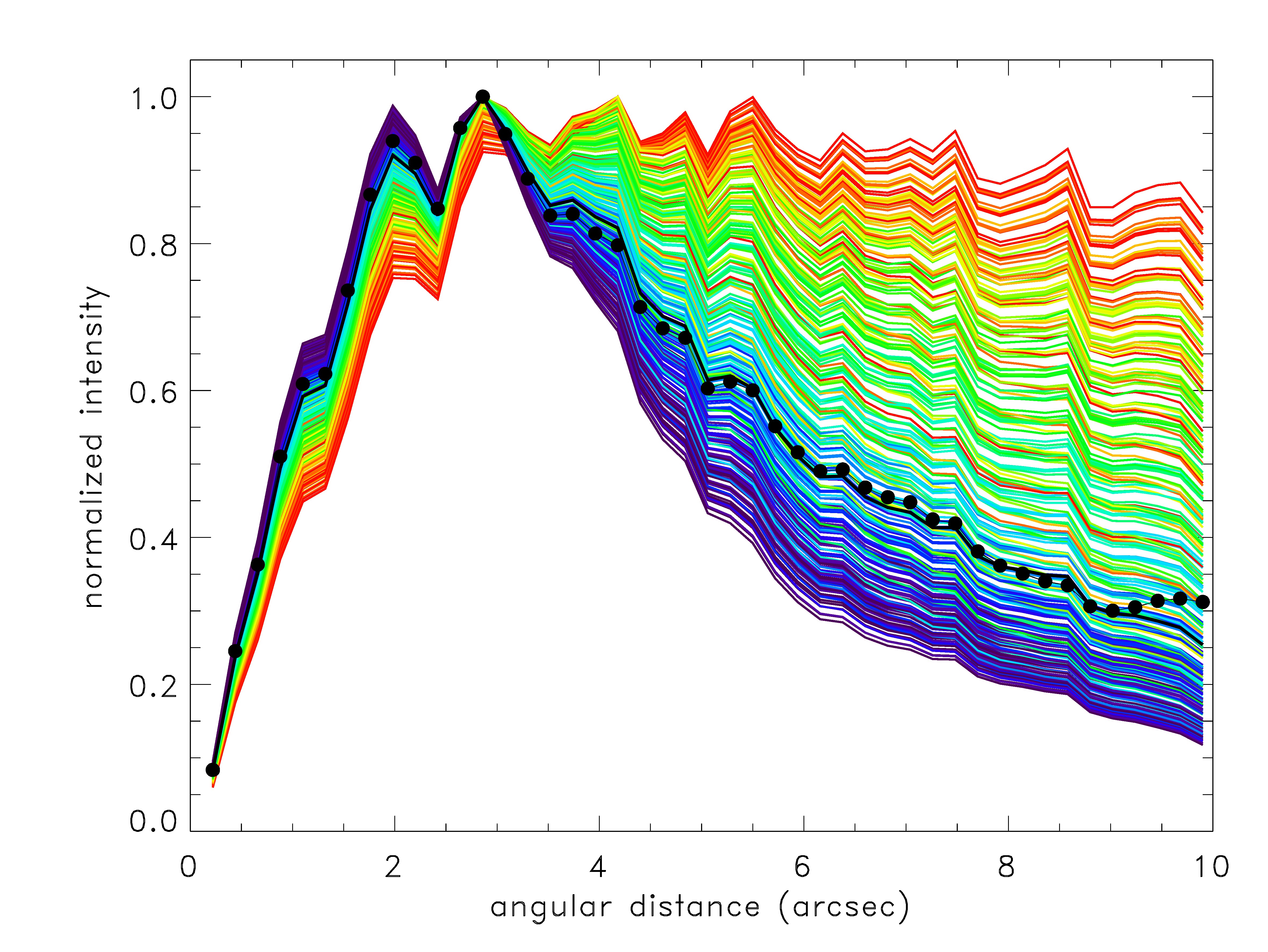
Figure 3: Normalised intensity profiles of various model settings (coloured curves). Curves with colours from blue to red correspond to size distribution parameters from q = –1.6 to –3.0. The observed intensity profile is marked by black dots. The ”best fit” (lowest $\chi^{2}$) curve (solid line) corresponds to a model setting of t₀ = 1.6$\cdot$10⁷ s, v_ref = 1.0 m s^-1 and q = –2.0.

6 Summary

Here we have reported on the thermal infrared observations of comet C/2013 A1 performed with the Herschel Space Observatory at a heliocentric distance of 6.48 au. The comet showed an active coma, detected in all PACS photometric bands (70, 100 and 160 $\mu$m). Using simple calculations based on the observed thermal emission we obtained a dust production rate of 1.5$\pm$0.5 kg s^-1, and an $Af\rho$ value of 185$\pm$25 cm, indicating a slow increase, unusual for an Oort cloud comet. The total dust mass of the coma is estimated to be $\sim$3$\cdot$10⁸ kg. A more detailed dust grain model suggests that large grains are overabundant in the coma. Our model also indicates that the activity likely started close to a heliocentric distance of 8 au.

Appendix A Appendix

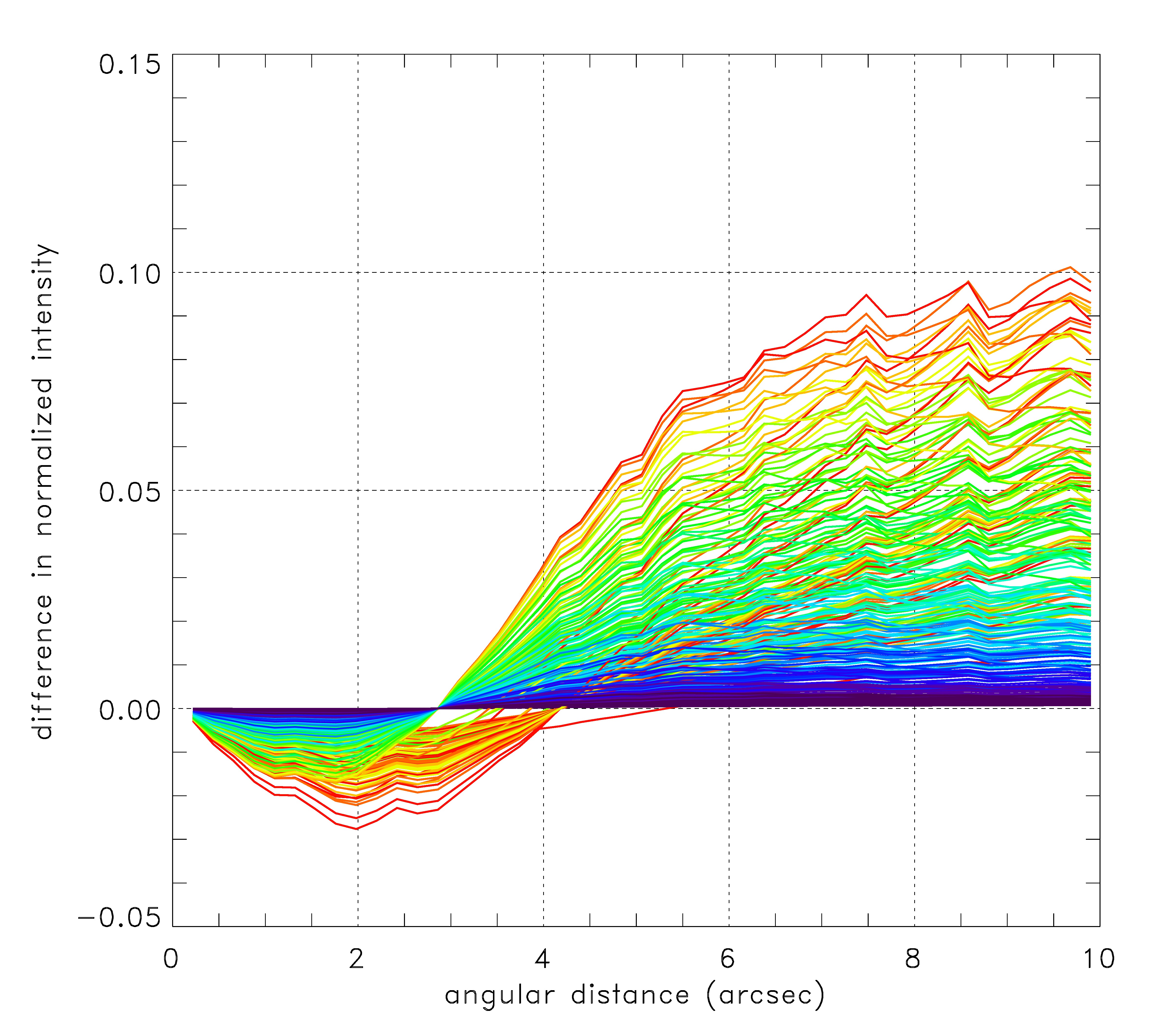
Figure 5: Difference of the astrosilicate and carbon particle dust emission model intensity profile curves using the same input parameters (t₀, v_ref and $q$). Curves with colours from blue to red correspond to size distribution parameters from q = –1.6 to –3.0, as in Fig. 3