Localization in a spanwise-extended model of plane Couette flow
Abstract
We consider a 9-PDE (1-space and 1-time) model of plane Couette flow in which the degrees of freedom are severely restricted in the streamwise and cross-stream directions to study spanwise localisation in detail. Of the many steady Eckhaus (spanwise modulational) instabilities identified of global steady states, none lead to a localized state. Localized periodic solutions were found instead which arise in saddle node bifurcations in the Reynolds number. These solutions appear global (domain filling) in narrow (small spanwise) domains yet can be smoothly continued out to fully spanwise-localised states in very wide domains. This smooth localisation behaviour, which has also been seen in fully-resolved duct flow (Okino 2011), indicates that an apparently global flow structure needn’t have to suffer a modulational instability to localize in wide domains.
I Introduction
The transition to turbulence in wall-bounded shear flows is an old and intriguing problem in fluid dynamics since transition is typically observed even though the laminar state is stable. The discovery in the last twenty years of exact but unstable solutions (e.g. Nagata (1990); Waleffe (1998); Faisst & Eckhardt (2003); Wedin & Kerswell (2004)) surrounding the laminar state in phase state has helped explain how transitional flows can be so complicated. Progress continues to be made using the growing library of solutions and ideas from dynamical systems theory to understand the dynamics as a walk in phase space between such solutions (Kerswell & Tutty, 2007; Gibson et al., 2008; Kawahara et al., 2012; Willis et al., 2013; Kreilos et al., 2014). However computational limitations have restricted much of this work to small domains periodic in space where turbulence is global. Extending this approach to physically-realised domains requires localized solutions.
The first of these - a solution localized in the spanwise direction - was found via edge tracking by Schneider et al. (2010b) in plane Couette flow (pCf). Perhaps more important was the discovery via continuation in Reynolds number of the connection of the localized solution branch to a bifurcation from a spatially-periodic solution (Schneider et al., 2010a). This opened up the possibility of using the catalogue of known spatially-global solutions to find localized versions. However, edge tracking has continued to be the method of choice (e.g. in pipe Avila et al. (2013); Chantry et al. (2014); channel flow Zammert & Eckhardt (2014b, a) and pCf Melnikov et al. (2014)) with subsequent connections found only later moving from the localized solutions to global solutions Chantry et al. (2014).
One novel approach to going from spatially-periodic states to localised states has been to attempt to converge cleverly-masked versions of global solutions as localised solutions of the governing equations Gibson & Brand (2014); Brand & Gibson (2014). While successful, this has not informed the important question of how generic bifurcations are which lead to localized solutions when viewed amongst all the bifurcations experienced by the spatially periodic solutions. The numerical cost of finding and tracking bifurcations in the large domains necessary to see localisation, makes seeking an answer an intimidating proposition. Nevertheless Melnikov et al. Melnikov et al. (2014) have made a start by studying long spanwise wavelength instabilities of one global state in pCf. However, they did not show how such bifurcations could lead to a localised state although edge tracking indicated localised states did exist nearby. The motivation for this study was to introduce a more-accessible low-dimensional model to explore the result of bifurcations from spanwise-periodic states and the existence of localised states. A particular objective was to see if the homoclinic snaking (Champneys, 1998; Burke & Knobloch, 2007; Chapman & Kozyreff, 2009) seen in Schneider et al. (2010b) could be captured here.
Low-dimensional models have been employed in the past to try to understand facets of turbulent shear flows with a good track record of success. Waleffe Waleffe (1997) constructed a hierarchy of models for pCf consisting of ordinary differential equations (ODEs) describing the evolution of prescribed flow modes representing the crucial flow ingredients observed in experiments. He demonstrated that a self-sustaining process could transfer energy between the mean flow, rolls, streaks and wave-like instabilities in a cycle but these simple models could not reproduce the complex temporal dynamics of turbulence. Moehlis et al. Moehlis et al. (2004) adapted Waleffe’s 8-ODE model to include higher harmonic interactions by adding a further ODE. This 9-ODE model showed many of the rich temporal dynamics of turbulence with sensitivity to initial conditions, memoryless decay and exact solutions (Moehlis et al., 2005). Dawes and Giles Dawes & Giles (2011) carried out a different extension of the 8-ODE model by removing the prescribed spanwise dependence of the modes leading to 8 PDEs in the spanwise coordinate, , and time . This extension also generated a model with many of the characteristics of turbulence but the focus was on spanwise-limited (narrow) domains. In this work we combine these two extensions to study a 9-PDE extension of the 9-ODE model over spanwise-extended (wide) domains to examine how the flow can spanwise-localise. This 9-PDE model, which restricts the dynamics in 2 spatial directions but fully resolves the remaining spanwise direction, is similar in spirit to previous reduced models which fully resolve 2 spatial directions and use a reduced resolution in the other Manneville & Locher (2000); Manneville (2014); Lagha & Manneville (2007); Willis & Kerswell (2009). If (Willis & Kerswell, 2009) described their model as a ‘2+’ dimensional model, then our model here is ‘1+2’ dimensional.
This paper is organized as follows. Section II (supported by Appendix A) describes the derivation of the reduced model which is closely related to the 8-PDE model of Dawes & Giles (2011), and briefly discusses the spatial Floquet theory employed to identify the Eckhaus (modulational) instabilities of interest here. Section III details the spanwise-periodic states found in the model, the steady modulational instabilities they possess and the results of tracking all of these bifurcations. Section IV applies edge tracking to find localized solutions and section V explores the effect of different spanwise boundary conditions. A final section discusses our results and their implications for fully-resolved models of the wall-bounded shear flows.
II Model derivation
 0
0
To study spanwise localization processes, a set of 9 PDEs in and are derived with the various steps closely following Dawes & Giles (2011). Plane Couette flow is the flow between two parallel plates moving in their plane in opposite directions. The coordinate system is defined with in the downstream direction, in the shear-dependent direction and in the spanwise direction. The Navier-Stokes equation is non-dimensionalized by , the half distance between the walls and the laminar flow speed at (this differs from pCf where wall speed is used). The Reynolds number in this system is defined as , where is the kinematic viscosity. In sections III and IV, we consider a domain periodic in and with impermeable, stress-free boundary conditions in (in section V, the boundary conditions in are changed to non-slip). For these conditions are written as
| (1) | |||
| (2) |
The dimensions of the domain are . The system is driven by the body force,
where . This results in a steady unidirectional laminar flow
This forcing was chosen by Waleffe to produce a base flow close to that of pCf but using Fourier modes. Despite the inflection point this flow remains linearly stable for all Reynolds numbers (Drazin & Reid, 1981, page 132).
II.1 Model derivation
To derive the model we begin with the 9-mode ansatz of Moehlis et al. (2004) but remove the prescribed -dependence. Following Dawes & Giles (2011) these modes are rewritten in a mean, toroidal and poloidal form,
where these components are defined as
leading to
| (3) |
where
The Moehlis adaptation introduced , adding variation in to the base profile, and included terms capturing additional nonlinear interactions and linking the new mode. These modes can be divided into four categories representing the self-sustaining process introduced by Waleffe (1997). Modes generated by and represent the mean profile and variation of the mean profile; represents the downstream streaks which are generated by the roll mode ; finally the self-sustaining cycle is closed using five wave-like instability modes .
Individual evolution equations for the are formed by taking a Galerkin projection of the Navier-Stokes equations (or its curl) in and . The resulting equations have general form
| (4) |
where and are linear operators, is a quadratic nonlinear operator and is the constant forcing term (see appendix A for details). The nonlinear terms conserve energy as in the Navier-Stokes equations.
II.2 Symmetries
Symmetries play an important part in this work and the system (4) has several symmetry subspaces. The most important to the dynamics of this model is inherited from the predecessor models of Waleffe and Moehlis. This symmetry prescribes the following -dependence on the modes
| (5) |
which means , with all other unchanged and therefore not shown. Physically, represents the flow field symmetry
| (6) |
for the -independent mean flow modes and
| (7) |
for the -dependent instability modes but has no equivalent symmetry in the Navier-Stokes equations. In this Waleffe system, the symmetry stems from choosing a roll symmetry, considering the streaks thus generated and the optimal instability to close the system. Equation (4) is also invariant under two transformations and two shifts
| (8) | ||||
| (9) | ||||
| (10) | ||||
| (11) |
which correspond to the following mode operations
| (12) | ||||
| (13) | ||||
| (14) | ||||
| (15) |
Spatially, the system is solved using a pseudospectral method based upon a Fourier series for periodic boundary conditions in sections III and IV and Chebyshev polynomials in section V for non-slip sidewalls. Typical resolutions are 10 Fourier modes per length in the spanwise direction so that, for example, a steady state in a wide domain has 900 degrees of freedom (reduced to 450 by symmetry) and a periodic orbit three times this. The equations are time-stepped using Crank-Nicolson method for the linear terms and a 2nd order Adams-Bashforth method for the nonlinear terms. Convergence and continuation of simple invariant sets (e.g. steady states and periodic orbits) was carried out using PITCON (Rheinboldt & Burkardt, 1983).
II.3 Spatial Floquet theory
Starting with a spatially periodic state
| (16) |
which has the discrete spatial symmetry (where is the solution wavenumber), disturbances of the form
| (17) |
(where denotes the complex conjugate and thus is real) were considered in order to uncover Eckhaus (modulational) bifurcations associated with localization These disturbances have a wavelength of which is times longer than the underlying spatially-periodic state. Only steady bifurcations, indicated by passing through 0, were tracked since these were plentiful enough. For -odd, two branches of solution can emanate out of a bifurcation, corresponding to for near the bifurcation point. For -even, these two branches are related by the broken shift symmetry,
| (18) | ||||
There still are 2 branches but they are related by the simple application of .
III Steady states and steady modulational instabilities


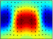
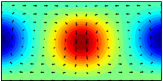
To find spatially-periodic solutions from which to study modulational instabilities, the 9-PDE model was simulated at , & in a narrow domain where global, long-lived chaotic behaviour is present. Velocity fields every 500 time units were then used as initial conditions in a Newton solver (this ‘shooting in the dark’ method was only feasible due to the simplicity of the model). Using this approach, three steady solutions were identified - hereafter , and - all possessing symmetry: see figure 2. Each solution was discovered at a Reynolds number just above their saddle node, with both upper and lower branches lying in the chaotic saddle. Beyond these Reynolds numbers, the solutions could no longer be found using this method due to their increasing instability.
Re
Steady modulational bifurcations from these -symmetric spatially-periodic states were then searched for. These bifurcations differ subtly from those in the Swift-Hohenberg equations and the snaking solutions of Schneider et al. (2010a). The periodic solutions in both these latter settings have two planes of spanwise symmetry with symmetry about and antisymmetry about which together generate . Bifurcating solutions breaking must then break one of these reflectional symmetries, generating two solutions, one in each symmetry subspace. Here, the symmetry is not generated by plus a second symmetry plane and therefore generically modulational bifurcations will remain in the subspace of . Ideally, we should search for bifurcations from a solution with two symmetry planes, however no such solutions were found in this model.
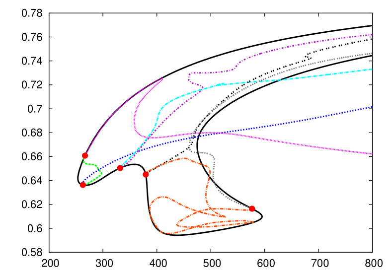
The solution branches emanating from all steady bifurcations with modulation number from the underlying solution branch, , are shown in figure 3: the energy, , defined as
| (19) |
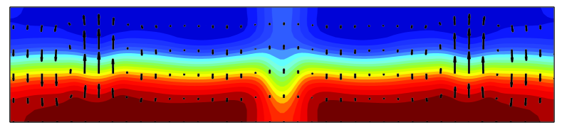
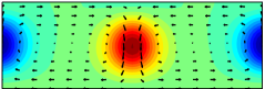
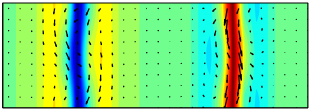
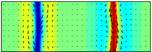
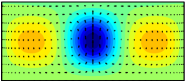
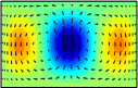
is plotted against Re. There are five bifurcations with each producing two solution branches and their behaviour falls into two categories: either reconnecting at an alternate bifurcation point, or continuing to large Re. In neither case do the solutions localize let alone snake. A typical solution at large Re is plotted in figure 4 demonstrating the non-trivial flow throughout the domain (note the aspect ratio of the plots which cause the transverse velocities to all appear essentially perpendicular to the boundaries).

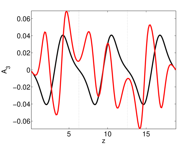
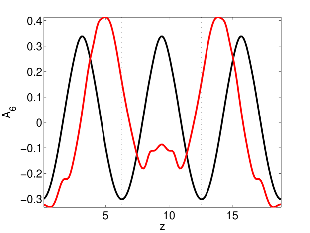
It is instructive to compare the structure of the bifurcating eigenfunction with the individual modes in the model at one typical modulational bifurcation. Figure 5 plots & , which represent the rolls and a roll instabilities respectively for the underlying solution branch (black), and the modulational (M=3) instability closest to the saddle-node (, in red). The eigenfunction is in phase with in the centre of the domain, and out of phase at the edges of the domain, whereas for the opposite is true. Therefore close to the bifurcation these modes cannot both act to diminish their respective modes at the same point in the domain, moving towards a localized solution. This conflicting behaviour of modes is observed for all of the bifurcations tracked and helps explain why these bifurcations do not lead to localization.
Widening the search, steady modulational instabilities with were sought for , & . All bifurcating solution branches found, however, follow the two behaviours outlined above, with no evidence of localization. It was found that bifurcations for were all of a similar type existing close to one another on the solution curve, as illustrated in figure 6. Since no localization was found, the focus was shifted to consider wider domains to extract localized solutions using a different approach.

Re
IV Localization in wide domains
In this section, a different strategy was adopted for generating localised solutions by considering solutions embedded within the edge. The edge is a hypersurface that separates initial conditions which become turbulent from those which simply relaminarize (Itano & Toh, 2001; Skufca et al., 2006; Schneider et al., 2007) and can be considered a generalization of the basin boundary for the laminar state to systems where turbulence is not an attracting state. Despite the unstable nature of this surface, a bisection technique can be used to track the dynamics within this surface. Tracking these dynamics in the various shear flows has been an effective way to simplify the dynamics and can lead to exact solutions that are stable within the surface. In pCf, pipe flow and channel flow, this technique has revealed global solutions (Schneider et al., 2008; Duguet et al., 2008) and the first exact localized solutions (Schneider et al., 2010a; Avila et al., 2013; Chantry et al., 2014; Zammert & Eckhardt, 2014b, a).
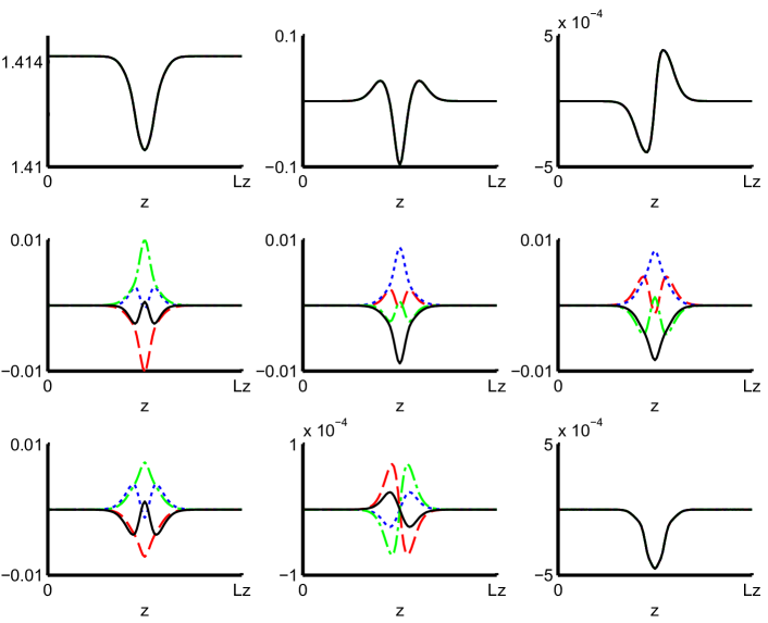
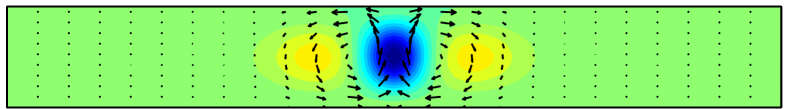
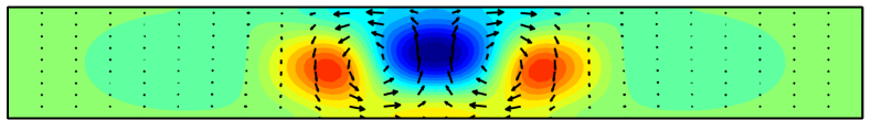
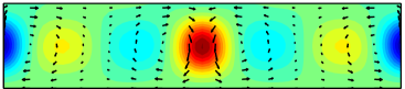
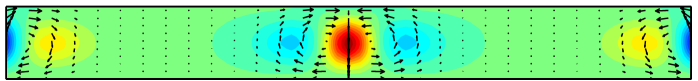
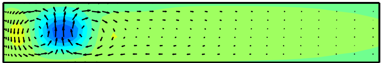
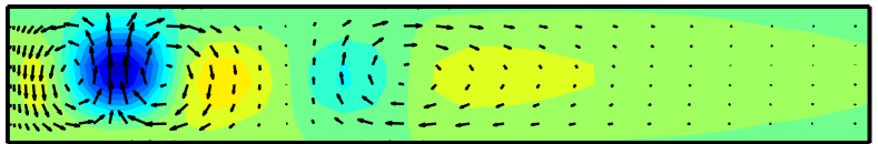
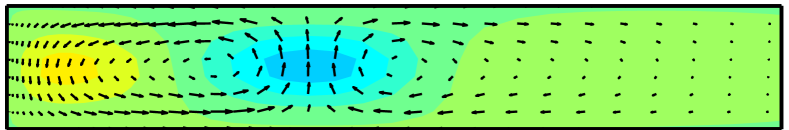
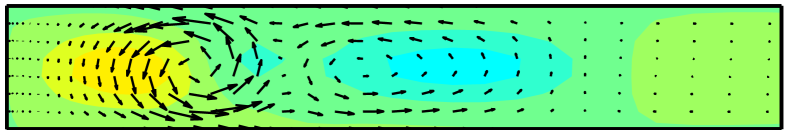
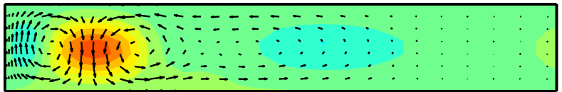
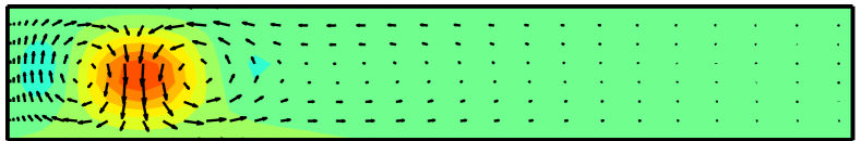
Edge-tracking in a wide domain (5 times wider than in section III) at leads to a spanwise-localized periodic orbit (hereafter called ‘P1’) depicted in figure 7. This solution has a short period () with a spatiotemporal symmetry
| (20) | ||||
Working with the general representation
| (21) |
the structure of the equations is such that the -independent modes of only possess even powers of and -dependent modes only odd powers, that is,
| (22) | ||||
| (23) |
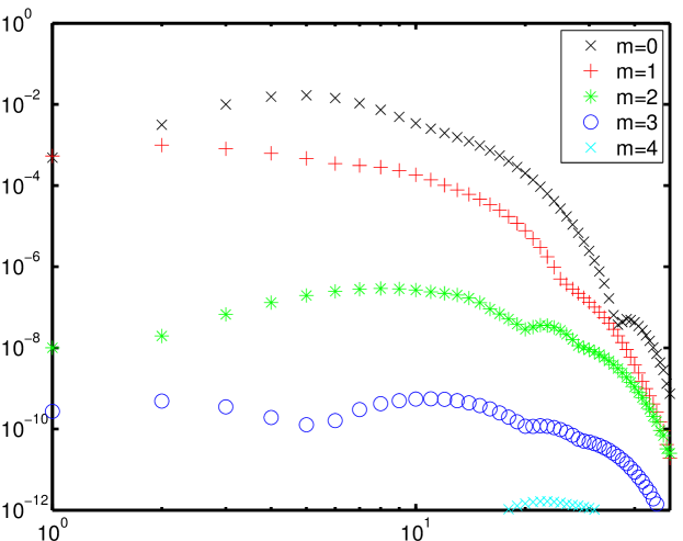
Moreover, the rapid decay of the temporal spectrum - see figure 8 - actually allows for the convergence and accurate continuation of using the extreme temporal truncation
| (24) |
is also -symmetric which was not imposed during the edge tracking procedure.
(a)
Re
(b)
(c)
(b)
LB
(c)
UB
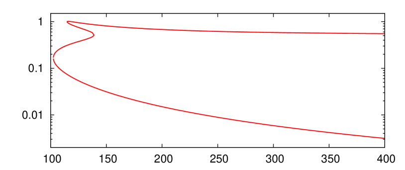
The localized solution of Schneider et al. (2010a) in plane Couette flow was found to undergo ‘snaking’ where the localized solution branch passes through a series of folds with each fold adding a wavelength to the solution pattern before the domain is filled whereupon a connection is reached to a spanwise-periodic state. (This behaviour was originally studied in the Swift-Hohenberg equations (Champneys, 1998; Burke & Knobloch, 2007; Chapman & Kozyreff, 2009) and has recently been discovered in other fluid problems (Lo Jacono et al., 2010; Beaume et al., 2011)). To look for snaking behaviour here, was continued in Re as shown in figure 9 where the time-averaged energy
| (25) |
is plotted. The continuation curve undergoes 3 saddle-node bifurcations close to the minimum Reynolds number in a manner similar to snaking curves. However the curve turns back towards larger values of Re and while some structure is added during the continuation from lower to upper branch the additional structure does not match the amplitude of the central pattern. Reintroducing higher temporal harmonics confirmed these continuation results.
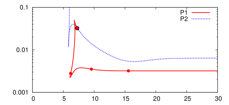
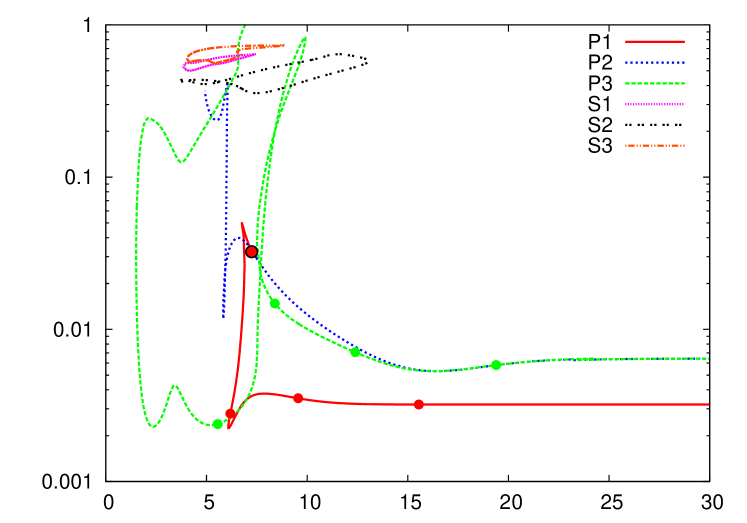
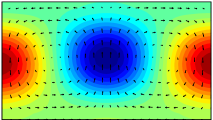
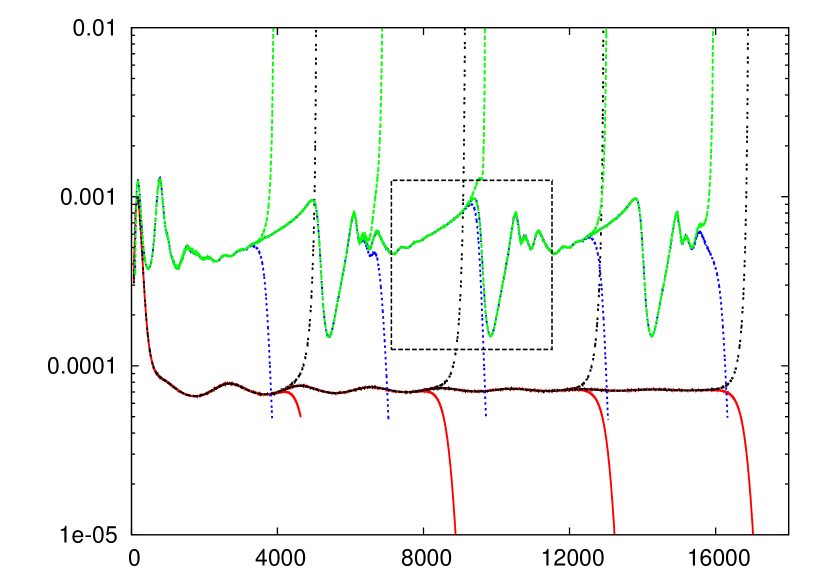
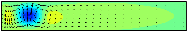
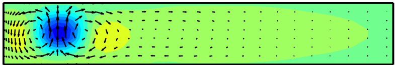
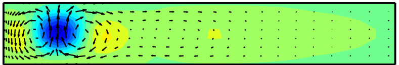
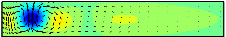
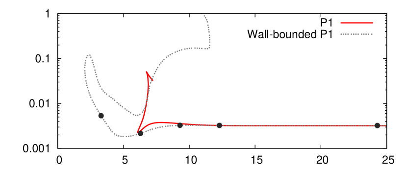
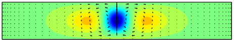
Fixing Re at 400 and continuing to smaller spanwise domain sizes - see the solid red curve in figure 10 - reveals that only starts to feel the spanwise domain size at . Below this value, undergoes a saddle node bifurcation at , after which the time averaged energy rapidly increases until meets a more symmetric state P2 at (the solution evolution as a function of is depicted in figure 11). has the symmetry which is broken at to give .
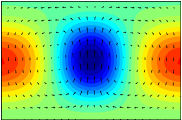
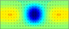
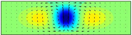
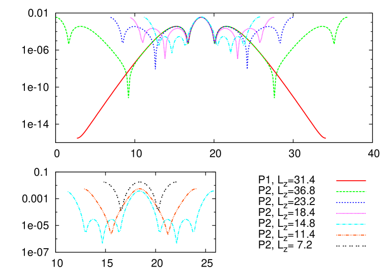
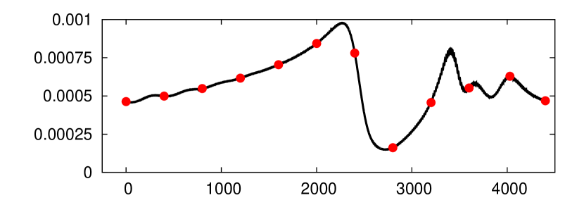
Continuing this new symmetric solution towards larger values of results in 2 copies of , related by and separated by . Figure 12 shows the time-averaged energy density as a function of spanwise position
| (26) |
For increasing domain widths each localized part of the solution matches the spatial structure of with exponential decay towards the laminar state at its spanwise extremities ( has an unstable eigenvalue of multiplicity two and is therefore unstable within the edge). experiences a saddle node at and moving onto the upper branch the simple temporal ansatz (24) begins to break down as higher temporal harmonics become significant. Figure (10) seems to indicate that might connect directly to one of the three global states or but the structure of P2 actually precludes this. In all the time-periodic solutions found, the -dependent modes are purely time dependent, with no time-independent part. Since these modes are necessary for non-trivial solutions, the periodic solutions cannot be borne directly in a Hopf bifurcation from a steady state. The -dependent modes would first have to develop a time-independent component before the time-dependent part could go to zero. For these and computational reasons we did not track the solution branch further on the upper branch.
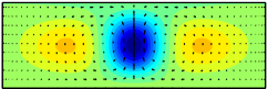
Edge tracking in smaller domains () reveals a new domain-filling periodic orbit, as the edge state (see figures 10(b) and 13). The solution has simple temporal structure and two symmetries and . Continuing this solution to large domains (dashed green curve in figure 10) the branch briefly becomes more energetic before stretching out to produce another localized pair of the periodic orbit this time with each component being related to the other via the symmetry .
Localized solution pairs ( symmetric) and ( symmetric) differ only in the downstream position (or equally, the phase in the time period,) of one of the individual localized solutions which make up the pair. The transformation
| (27) |
where one localized solution lies in each region, maps one solution pair to another. This is depicted in figure 14 where the two solutions are plotted in plane. This difference in the phase between the two solutions for large becomes significant as decreases because the two subcomponents are brought together leading to different global states.
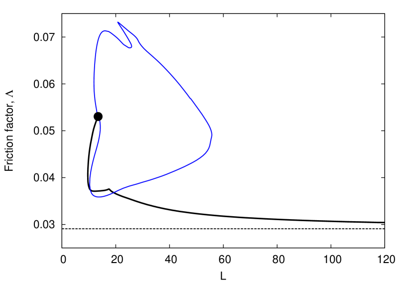
The behaviour of the solutions , and to smoothly move between an apparently ‘global’ state and a localized structure as the spanwise domain is changed runs counter to the usual expectation that there should be a bifurcation between these two extremes. For example, the localizing states found via edge tracking in Melnikov et al. (2014) (see their figure 11 (b) and (c)) are the results of a modulational instability from a global travelling wave state (see their figure 6 and 11(a)). One explanation is that a localised solution appears to become global near to where it connects to a global branch of solutions as in Chantry et al. (2014). Figure 15 replots the inset of figure 1 in Chantry et al. (2014) to show the localised (black) branch going through a turning point (corresponding to the minimum domain size) before connecting to the closed (blue) global branch in a slightly larger domain (localization here is in the streamwise rather than spanwise direction). At this turning point, the flow on the localised branch looks domain filling. However, the localised states in our model are not connected to any global state at the Reynolds numbers considered and there are structural reasons to expect there not to be such a connection at all (the -dependent modes have no steady part). The fact that this behaviour has also been seen in the preliminary work of Okino (2011, page 89, fig 5.1) on rectangular duct flow indicates that this observation is not an artefact of the model. In Okino (2011), a (global) travelling wave solution found in a square duct was smoothly continued to wide aspect-ratio ducts to reveal a spanwise-localised travelling wave with very little adjustment in the structure from the square duct situation. One difference between the work here and Okino’s calculation is the spanwise boundary conditions imposed: periodic here and no-slip there. It is worth confirming that this is not significant.
V Spanwise walls
The periodic spanwise boundary conditions are replaced in this section by no-slip conditions on the deviations from the laminar flow,
which means the modes satisfy the following conditions
| (28) | ||||
| (29) | ||||
| (30) |
The equations are solved using a Chebyshev collocation method. Searching for localization, a domain of size is considered at Reynolds number 400. In a domain of these dimensions the localized periodic orbit, , (see frame 1 of figure 11) is an edge attractor both for periodic and no-slip boundary conditions. However, while evidence suggests that the periodic orbit is the unique attractor for periodic boundary conditions, this is not true for no-slip conditions. In this domain, in addition to a second solution, , attracts the dynamics within the edge. The energetic evolution of two initial conditions in the edge is plotted in figure 16, where the two initial conditions were generated from turbulent initial conditions separated by 30 time units. This new solution, , attracts the dynamics when the fluctuations are strong near one of the wall regions and the dynamics along the orbit are shown in figure 17. Evidence from edge tracking suggests that the solution is a periodic orbit where the state after half a period () is related to the initial state through spatial-temporal symmetry
| (31) |
However, the extremely long period of the structure prevents convergence of the solution. Within the slow time-scale behaviour the -dependent modes oscillate on a time-scale of 24 units throughout the period (not visible in figure 17). Ignoring the long-timescale dynamics these oscillations take a similar form to those exhibited by the temporally-simple localized periodic orbit with
The transition from quiescent evolution (the first seven snapshots in figure 17) to fast evolution (the last five snapshots), suggest the solution may be an analog of the bursting solutions of van Veen & Kawahara (2011); Khapko et al. (2013).
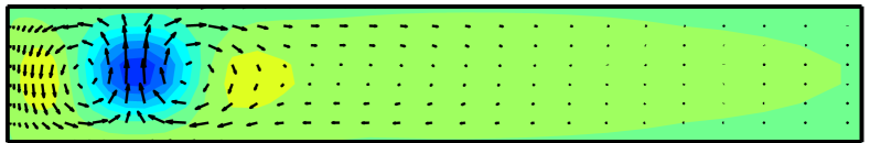

Finally, we consider the continuation of solution with spanwise-walls imposed (figure 18). For domains of width the solution is indistinguishable from the periodic boundary condition equivalent. Below this value the fast streaks (yellow) are squashed by the incoming walls, while the central slow streak (blue) remains unaltered so that the smooth transition between localized and domain filling solution is again recovered. Beyond the saddle-node, the time complexity increases along the upper branch and the solutions were not tracked.

VI Conclusions
In this work we have derived a 9-PDE extension to the 9-ODE Moehlis model (Moehlis et al., 2004) in order to study spanwise localization. Despite tracking many steady modulational bifurcations from 3 different global steady states, we found no tendency for localization and therefore also no instance of homoclinic snaking. Localized periodic orbits can, however, be found by edge-tracking. When smoothly continued to smaller spanwise domains, these look like global states as they fill the domain but are not connected via any bifurcation to global states which only exist for a finite range of domain sizes (e.g. figure 15). This behaviour is not dependent on the exact form of the spanwise boundary conditions as it persists when no-slip sidewalls replace spanwise periodicity.
The conclusions to be drawn from this model study are therefore twofold: a) modulational instabilities leading to localisation from global states are not generic at least when only considering steady flows; and b) localized solutions can smoothly morph into global solutions (and vice versa) without any need for a bifurcation in between. This smooth local-to-global transition has not as yet been observed in plane Couette flow but has been in fully resolved computations in duct flow Okino (2011). There, a square duct travelling wave solution could be continued to a much wider domain with little change to solution structure.
In terms of future work, the challenge still remains (surprisingly) to demonstrate the generation of a localised state from a global state by following a modulational instability in the Navier-Stokes equations. The few such bifurcations known have so far only be found in ‘reverse’ by tracking a localised solution back to its global cousin Schneider et al. (2010b); Chantry et al. (2014). The work reported here has also highlighted the fact that localized solutions may not be connected to any global states which only exist over a finite range of domain sizes. Instead, they may be simply borne in a saddle node bifurcation as the domain size increases. Finally, we note that the modelling strategy adopted here to develop a spanwise-extended system could also equally be used to build a streamwise-extended model of 1-space and 1-time PDEs. This smooth local-to-global transition may well also exist for streamwise localisation too.
Acknowledgements. Matthew Chantry is very grateful for the support of EPSRC during his PhD.
Appendix A Model Derivation
The evolution equations for the modes listed in (3) are derived using Fourier orthogonality in the and directions. To simplify notation we introduce the following
To derive the equation for (, ) we take the
component of the Navier-Stokes, multiply this by the
component of (, ) and integrate over
and ,
| (32) |
| (33) |
| (34) |
To generate the equations for modes 3-7 we consider the curl of the Navier-Stokes,
| (35) |
| (36) |
| (37) |
| (38) |
| (39) |
Finally, we take the curl twice to produce the evolution equation for ,
| (40) |
References
- Avila et al. (2013) Avila, M, Mellibovsky, F, Roland, N & Hof, B 2013 Streamwise-localized solutions at the onset of turbulence in pipe flow. Physical Review Letters 110 (22), 224502.
- Beaume et al. (2011) Beaume, Cedric, Bergeon, Alain & Knobloch, Edgar 2011 Homoclinic snaking of localized states in doubly diffusive convection. PHYSICS OF FLUIDS 23 (9).
- Brand & Gibson (2014) Brand, E. & Gibson, J.F. 2014 A doubly localised equilibrium solution of plane couette flow. J. Fluid Mech. 750, R3.
- Burke & Knobloch (2007) Burke, John & Knobloch, Edgar 2007 Homoclinic snaking: structure and stability. Chaos: An Interdisciplinary Journal of Nonlinear Science 17 (3), 037102–037102.
- Champneys (1998) Champneys, AR 1998 Homoclinic orbits in reversible systems and their applications in mechanics, fluids and optics. Physica D: Nonlinear Phenomena 112 (1), 158–186.
- Chantry et al. (2014) Chantry, M., Willis, A. P. & Kerswell, R. R. 2014 Genesis of streamwise-localized solutions from globally periodic traveling waves in pipe flow. Phys. Rev. Lett. 112, 164501.
- Chapman & Kozyreff (2009) Chapman, SJ & Kozyreff, Gregory 2009 Exponential asymptotics of localised patterns and snaking bifurcation diagrams. Physica D: Nonlinear Phenomena 238 (3), 319–354.
- Dawes & Giles (2011) Dawes, Jonathan HP & Giles, WJ 2011 Turbulent transition in a truncated one-dimensional model for shear flow. Proceedings of the Royal Society A: Mathematical, Physical and Engineering Science 467 (2135), 3066–3087.
- Drazin & Reid (1981) Drazin, PG & Reid, WH 1981 Hydrodynamic stability, p. 132.
- Duguet et al. (2008) Duguet, Yohann, Willis, Ashley P & Kerswell, Rich R 2008 Transition in pipe flow: the saddle structure on the boundary of turbulence. Journal of Fluid Mechanics 613 (1), 255–274.
- Faisst & Eckhardt (2003) Faisst, Holger & Eckhardt, Bruno 2003 Traveling waves in pipe flow. Physical review letters 91 (22), 224502.
- Gibson & Brand (2014) Gibson, JF & Brand, E 2014 Spanwise-localized solutions of planar shear flows. Journal of Fluid Mechanics 745, 25–61.
- Gibson et al. (2008) Gibson, J. F., Halcrow, J. & Cvitanovic, P. 2008 Visualizing the geometry of state space in plane Couette flow. Journal of Fluid Mechanics 611, 107–130.
- Itano & Toh (2001) Itano, Tomoaki & Toh, Sadayoshi 2001 The dynamics of bursting process in wall turbulence. Journal of the Physics Society Japan 70 (3), 703–716.
- Kawahara et al. (2012) Kawahara, G., Uhlmann, M. & van Veen, L. 2012 The significance of simple invariant solutions in turbulent flows. Ann. Rev. Fluid Mech. 44, 203–225.
- Kerswell & Tutty (2007) Kerswell, R.R. & Tutty, O.R. 2007 Recurrence of travelling waves in transitional pipe flow. J. Fluid Mech. 584, 69–102.
- Khapko et al. (2013) Khapko, Taras, Kreilos, T, Schlatter, Philipp, Duguet, Y, Eckhardt, B & Henningson, Dan Stefan 2013 Localized edge states in the asymptotic suction boundary layer. Journal of Fluid Mechanics 717, R6.
- Kreilos et al. (2014) Kreilos, T., Eckhardt, B & Schneider, T.M. 2014 Increasing lifetimes and the growing saddles of shear flow turbulence. Phys. Rev. Lett. 112, 044503.
- Lagha & Manneville (2007) Lagha, M. & Manneville, P. 2007 Modelling transitional plane couette flow. Eur. Phys. J. B 58, 433–447.
- Lo Jacono et al. (2010) Lo Jacono, D., Bergeon, A. & Knobloch, E. 2010 Spatially localized binary fluid convection in a porous medium. PHYSICS OF FLUIDS 22 (7).
- Manneville (2014) Manneville, P. 2014 Spots and turbulent domains in a model of transitional plane couette flow. Theor. Comp. Fluid Dyn. 18, 169–181.
- Manneville & Locher (2000) Manneville, P. & Locher, F. 2000 A model for transitional plane couette flow. C.R. Acad. Sci. Paris 328, 159–164.
- Melnikov et al. (2014) Melnikov, Konstantin, Kreilos, Tobias & Eckhardt, Bruno 2014 Long-wavelength instability of coherent structures in plane couette flow. Physical Review E 89 (4), 043008.
- Moehlis et al. (2004) Moehlis, J., Faisst, H. & Eckhardt, B. 2004 A low-dimensional model for turbulent shear flows. New Journal of Physics 6, 56.
- Moehlis et al. (2005) Moehlis, J., Faisst, H. & Eckhardt, B. 2005 Periodic orbits and chaotic sets in a low-dimensional model for shear flows. SIAM J. Appl. Dyn. Syst 4, 352–376.
- Nagata (1990) Nagata, M 1990 Three-dimensional finite-amplitude solutions in plane couette flow: bifurcation from infinity. J. Fluid Mech 217, 519–527.
- Okino (2011) Okino, Shinya 2011 Nonlinear travelling wave solutions in square duct flow. PhD thesis, http://repository.kulib.kyoto-u.ac.jp/dspace/ bitstream/2433/142216/2/D_Okino_Shinya.pdf.
- Rheinboldt & Burkardt (1983) Rheinboldt, Werner C & Burkardt, John V 1983 A locally parameterized continuation process. ACM Transactions on Mathematical Software (TOMS) 9 (2), 215--235.
- Schneider et al. (2007) Schneider, Tobias M, Eckhardt, Bruno & Yorke, James A 2007 Turbulence transition and the edge of chaos in pipe flow. Physical review letters 99 (3), 34502.
- Schneider et al. (2010a) Schneider, Tobias M, Gibson, John F & Burke, John 2010a Snakes and ladders: Localized solutions of plane couette flow. Physical review letters 104 (10), 104501.
- Schneider et al. (2008) Schneider, Tobias M, Gibson, John F, Lagha, Maher, De Lillo, Filippo & Eckhardt, Bruno 2008 Laminar-turbulent boundary in plane couette flow. Physical Review E 78 (3), 037301.
- Schneider et al. (2010b) Schneider, Tobias M, Marinc, Daniel & Eckhardt, Bruno 2010b Localized edge states nucleate turbulence in extended plane couette cells. J. Fluid Mech. 646, 441.
- Skufca et al. (2006) Skufca, Joseph D, Yorke, James A & Eckhardt, Bruno 2006 Edge of chaos in a parallel shear flow. Physical review letters 96 (17), 174101.
- van Veen & Kawahara (2011) van Veen, Lennaert & Kawahara, Genta 2011 Homoclinic tangle on the edge of shear turbulence. Phys. Rev. Lett. 107, 114501.
- Waleffe (1997) Waleffe, Fabian 1997 On a self-sustaining process in shear flows. Physics of Fluids 9, 883.
- Waleffe (1998) Waleffe, F. 1998 Three-dimensional coherent states in plane shear flows. Phys. Rev. Lett. 81 (19), 4140--4143.
- Wedin & Kerswell (2004) Wedin, H & Kerswell, R R 2004 Exact coherent structures in pipe flow: travelling wave solutions. J. Fluid Mech. 508 (333-371), 2--5.
- Willis & Kerswell (2009) Willis, A.P. & Kerswell, R.R. 2009 Turbulent dynamics of pipe flow captured in a reduced model: puff relaminarization and localized ‘edge’ states. J. Fluid Mech. 619, 213--233.
- Willis et al. (2013) Willis, Ashley P, Cvitanovic, Predrag & Avila, Marc 2013 Revealing the state space of turbulent pipe flow by symmetry reduction. J. Fluid Mech. 721, 514--540.
- Zammert & Eckhardt (2014a) Zammert, Stefan & Eckhardt, Bruno 2014a A fully localised periodic orbit in plane poiseuille flow. preprint .
- Zammert & Eckhardt (2014b) Zammert, Stefan & Eckhardt, Bruno 2014b Periodically bursting edge states in plane poiseuille flow. Fluid Dynamics Research 46, 041419.