Instabilities and relaxation to equilibrium in long-range oscillator chains

Abstract

We study instabilities and relaxation to equilibrium in a long-range extension of the Fermi-Pasta-Ulam-Tsingou (FPU) oscillator chain by exciting initially the lowest Fourier mode. Localization in mode space is stronger for the long-range FPU model. This allows us to uncover the sporadic nature of instabilities, i.e., by varying initially the excitation amplitude of the lowest mode, which is the control parameter, instabilities occur in narrow amplitude intervals. Only for sufficiently large values of the amplitude, the system enters a permanently unstable regime. These findings also clarify the long-standing problem of the relaxation to equilibrium in the short-range FPU model. Because of the weaker localization in mode space of this latter model, the transfer of energy is retarded and relaxation occurs on a much longer time-scale.

The relaxation to equilibrium in nonlinearly coupled oscillators is still an open problem FPU ; galavotti . Starting with the pioneering work of Fermi-Pasta-Ulam-Tsingou (FPU) tod , these studies led to important discoveries in both statistical mechanics and nonlinear science. In most cases, the analysis was restricted to one-dimensional ($d=1$) lattices where oscillators interact only with nearest neighbors, i.e. to short-range interactions. However, in recent years there has been a growing interest in systems with long-range interactions long ; Campabook . In such systems, either the two-body potential or the coupling at separation $r$ decays with a power-law $r^{-\alpha}$. When the power $\alpha$ is less than the dimension of the embedding space $d$, these systems violate additivity, a basic feature of thermodynamics, leading to unusual properties like ensemble inequivalence, broken ergodicity, quasistationary states.

The extension of the FPU problem to include long-range couplings is rarely considered flach ; frac ; helena . Moreover, attention has been focused mainly on finding conditions for the existence of localized solutions like solitons or breathers. No one, to the best of our knowledge, has tackled, in the context of long-range systems, the original question posed by FPU on the time-scales for relaxation to equilibrium when the energy is fed into the lowest Fourier mode. This is the subject of this Letter. Moreover, we here show that the lessons learnt from the long-range FPU model can be used to clarify key features of the original short-range model.

Long-range coupled oscillator models have been previously introduced to cope with dipolar interaction in mechanistic DNA models dna . They describe also ferroelectric electr and magnetic magnet systems, where the long-range coupling is provided again by dipolar forces. Other candidates for application are cold gases: dipolar bosons trom ; atomdipol , Rydberg atoms rydberg , atomic ions kastner ; ions . Moreover, one can mention optical wave turbulence optics and scale-free avalanche dynamics ava , where such long-range couplings appear.

In this Letter, we consider a generalization of the FPU model by introducing a long-range coupling in the linear term, while keeping the nonlinear term short-range. Choosing the power $1<\alpha\leq 3$, the results do not depend much on the specific value. Dipolar systems correspond, as mentioned, to the power $\alpha=3$, while the power $\alpha=2$ has been considered for crack front propagation along disordered weak planes between solid blocks ava and contact lines of liquid spreading on solid surfaces liquid .

Here, we repeat the FPU experiment by putting the energy initially in the lowest Fourier mode. As for the short-range FPU model, an exponential spectrum involving only odd modes forms on a short-time scale ruffo ; flach1 . However, energy localization in Fourier space is much stronger, as we will comment in the following. By increasing the initial amplitude, a parametric instability sets in where the energy is transferred to even modes dri ; poggi ; chechin ; christo .

For the long-range FPU this instability has a sporadic nature, i.e. by increasing the amplitude one observes instability islands, narrow amplitude intervals where instability sets in. Similar sporadic instabilities (so called induction phenomenon ind ) have been observed in the short-range FPU when exciting higher modes. As we will show below, these instabilities play a much more important role in the long-range FPU than in the short-range one. This is due to the strong localization in mode space, which is ultimately determined by the non-equidistant character of the unperturbed frequency spectrum, see Fig. 1a. This instability drives the long-range system to energy equipartition on a short time-scale. For the short-range FPU, the simultaneous presence of sporadicity and weak localization in mode space, which is due to the equidistant character of the frequency spectrum shown in Fig. 1a, delays the convergence to energy equipartition. Therefore, the study of these instabilities for long-range systems clarifies an important aspect of the relaxation to equilibrium in the traditional short-range FPU model.

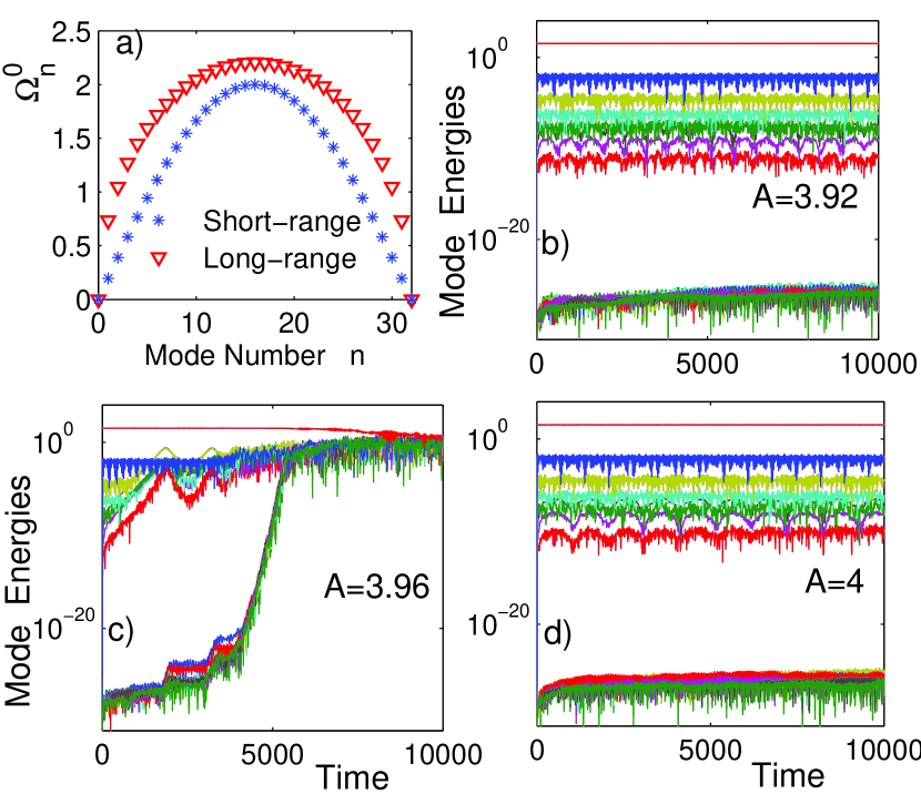
Figure 1: a) Unperturbed frequency distribution, $\Omega_{n}^{0}$ in formula 6, for the short-range FPU $\alpha=\infty$ (stars) and for the long-range one with $\alpha=2$ (triangles). b)-d) Time evolution of Fourier mode energies obtained by numerically integrating Eqs. (3). Initially, only the lowest mode is excited with increasing amplitudes: $A=1.96$, $A=1.98$ and $A=2$ (graphs b), c) and d), respectively). Warm colors (close to red) in b)-d) correspond to even modes while cold colors (close to green) represent odd ones. The number of oscillators in all panels is fixed to $N=32$ and the long-range interaction power is $\alpha=2$.

Let us consider the following long-range Hamiltonian, which describes a system of coupled nonlinear oscillators

$${\cal H}=\sum\limits_{{j=1}}^{N}\frac{\dot{u}_{j}^{2}}{2}+\sum_{j>\ell=1}^{N}{R_{j\ell}\frac{(u_{j}-u_{\ell})^{2}}{2}}+\sum\limits_{j=1}^{N}\frac{\left(u_{j+1}-u_{j}\right)^{4}}{4},$$ (1)

with displacements $u_{j}$ and velocities $\dot{u}_{j}$ of the $N$ oscillators. Quartic nonlinearity has been chosen so that the above model applies to the class of systems with inversion symmetry. We define the algebraically decaying interaction matrix elements of the harmonic term as

$$R_{j\ell}=\frac{1}{{\lvert j-\ell\rvert}^{\alpha}}+\frac{1}{(N-{\lvert j-\ell\rvert)}^{\alpha}},$$ (2)

in which $1<\alpha\leq 3$ is a long-range interaction power. The lower limit corresponds to a diverging harmonic interaction for infinite $N$ while, beyond the upper limit we are in the short-range regime flach . In order to be specific, we discuss here the case $\alpha=2$, but the results of simulations are similar for all long-range powers second .

Hamilton’s equations of model (1) are

$$\ddot{u}_{\ell}=\sum_{j=1}^{N}{R_{j\ell}}(u_{j}-u_{\ell})+\left(u_{\ell+1}-u_{\ell}\right)^{3}+\left(u_{\ell{-}1}-u_{\ell}\right)^{3}.$$ (3)

In momentum representation

$${Q}_{n}=\frac{1}{N}\sum_{\ell=1}^{N}u_{\ell}\,e^{iq_{n}\ell},$$ (4)

where $n$ is the normal mode number, and $q_{n}=2\pi n/N$, one can rewrite (3) in the following form

$$\ddot{Q}_{n}=-\left(\Omega_{n}^{0}\right)^{2}Q_{n}-\sum_{\langle m,r,p\rangle}^{N}G_{mrp}^{n}Q_{m}Q_{r}Q_{p},$$ (5)

where normal mode numbers satisfy the condition $m+r+p-n=0,N,2N,...$ and $\langle m,r,p\rangle$ further restricts the sum so that each triplet of modes $\{m,r,p\}$ is present only once. $G_{mrp}^{n}=D_{mrp}\omega_{m}\omega_{r}\omega_{p}\omega_{n}$ are mode coupling constants where $\omega_{r}\equiv 2\sin(q_{r}/2)$ and $D_{mrp}$ stand for the number of permutations of the set $\{m,r,p\}$, while $\Omega_{n}^{0}$ are unperturbed frequencies of the long-range normal modes

$$\Omega_{n}^{0}=\sqrt{2\sum_{m=1}^{N}\frac{1-\cos(q_{n}m)}{m^{\alpha}}}.$$ (6)

These frequencies are plotted in Fig. 1 for both a long-range and a short-range case. As mentioned above the spectrum is not equidistant in the long-range case. Originally, the FPU paradox involved exciting the first Fourier mode $n=1$ and looking for the equipartition of energy with respect to all other modes. Thus, we consider the following initial condition

$$u_{\ell}=A\left[e^{i(q_{1}\ell-\Omega_{1}^{0}t)}+c.c.\right]$$ (7)

which implies that energy is carried by normal modes $Q_{1}=A\,e^{i\Omega_{1}^{0}t}$ and $Q_{N-1}=\left(Q_{1}\right)^{*}$. In what follows we will study the evolution and instability of this initial excitation.

First of all, let us note that this mode could be treated, in the first approximation, as a source field and causes a nonlinear frequency shift to all normal modes. Indeed, examining nonlinear terms in (5) for $Q_{n}$ normal mode evolution containing $G_{n,1,N-1}^{n}Q_{n}Q_{1}Q_{N-1}$, we conclude that the expression for renormalized frequencies is

$$\Omega_{n}=\sqrt{\left(\Omega_{n}^{0}\right)^{2}+G_{n,1,N-1}^{n}\left|Q_{1}\right|^{2}}.$$ (8)

In addition, this source mode excites the branch of odd modes (often referred to as normal mode bush or q-breather chechin ; christo ; flach1 ). For instance, the initially absent $Q_{3}$ mode is generated according to the perturbation analysis of (5) $\ddot{Q}_{3}=-\left(\Omega_{3}^{0}\right)^{2}Q_{3}-G_{111}^{3}\left(Q_{1}\right)^{3}$ giving the exact solution

$$Q_{3}=\frac{G_{111}^{3}A^{3}}{9\Omega_{1}^{2}-\Omega_{3}^{2}}\left[e^{3i\Omega_{1}t}-\cos(\Omega_{3}t)-i\frac{3\Omega_{1}}{\Omega_{3}}\sin(\Omega_{3}t)\right].$$ (9)

Thus, in addition to the triple source harmonic $3\Omega_{1}$, $Q_{3}$ acquires the harmonic pair $\pm\Omega_{3}$ as well. In the long-range case, the perturbation analysis is well justified since low frequencies $\Omega_{j}$ are not equidistant, i.e. the ratio $(3\Omega_{1}-\Omega_{3})/\Omega_{1}$ remains finite even in the $N\rightarrow\infty$ limit, in contrast to the short-range FPU system. This itself guarantees the perturbative scaling $\left|Q_{1}\right|\gg\left|Q_{3}\right|$ and, as we will see below, leads to an excellent agreement between analytical predictions and numerical results. Proceeding further, we can derive perturbatively the expression for $Q_{5}$ with harmonics $\pm\Omega_{5}$, $\pm\Omega_{3}+2\Omega_{1}$ and $5\Omega_{1}$, and then for all odd normal modes which have exponentially decaying amplitudes with increasing mode number. We define such a steady distribution set of multicomponent and multi-frequency odd modes as $Q_{r}^{(a)}$, where $(a)$ indicates different harmonics of the $r$-th odd mode. Further, we should discuss how to derive the instability properties of this group of lowest energy modes.

First of all, we note that the initially excited lowest mode $Q_{1}$ alone (when all other modes are not excited) is parametrically stable in both long and short-range cases: thus, in order to analyze the instability process, it is necessary to consider the combination of odd modes created by the initial excitation of the first mode. Following a parametric instability approach, we consider pair of equations from the set (5)

$$\ddot{Q}_{n} = -\left(\Omega_{n}\right)^{2}Q_{n}-G_{mrp}^{n}Q_{m}Q_{r}^{(a)}Q_{p}^{(b)}$$ (10)

$$\ddot{Q}_{m} = -\left(\Omega_{m}\right)^{2}Q_{m}-G_{nrp}^{m}Q_{n}\left(Q_{r}^{(a)}\right)^{*}\left(Q_{p}^{(b)}\right)^{*},$$

where we have restricted the sum to mode harmonics such that the relative frequency

$$\Delta=\Omega_{r}^{(a)}+\Omega_{p}^{(b)}-\Omega_{m}-\Omega_{n},$$ (11)

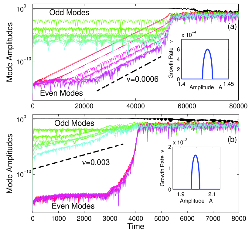
Figure 2: Long-range dynamics: Time dynamics of normal modes from numerical simulations on Eqs. (3) with initial mode amplitude $A=1.4225$ (graph a) and $A=1.97$ (graph b). Curves are color-coded according to the same principle as in Fig. 1. Insets show the dependence of growth rates on the initial lowest mode amplitude according to the theoretical formula (15). Dashed lines show the estimated grow rates for even (a) and odd (b) modes.

is close to zero. Then, introducing the transformations $Q_{n}={\cal Q}_{n}e^{i\Omega_{n}t}$ and $Q_{m}={\cal Q}_{m}e^{-i\Omega_{m}t}$, we get

$$\ddot{\cal Q}_{n}+2i\Omega_{n}\dot{\cal Q}_{n} = -G_{mrp}^{n}{\cal Q}_{m}{\cal Q}_{r}^{(a)}{\cal Q}_{p}^{(b)}e^{i\Delta t}$$ (12)

$$\ddot{\cal Q}_{m}-2i\Omega_{m}\dot{\cal Q}_{m} = -G_{nrp}^{m}{\cal Q}_{n}\left({\cal Q}_{r}^{(a)}\right)^{*}\left({\cal Q}_{p}^{(b)}\right)^{*}e^{-i\Delta t}.$$

The instability takes place when the approximate resonance condition $\Delta\approx 0$ holds. We can compute more precisely this threshold assuming a slow time evolution in (12) and neglecting second order time derivatives there. Thus, seeking for solution of the form

$${\cal Q}_{n}=F_{1}e^{(\nu+i\Delta/2)t}\quad\mbox{{and}}\quad{\cal Q}_{m}=F_{2}e^{(\nu-i\Delta/2)t},$$ (13)

with $F_{1}$, $F_{2}$ constants and real growth increment $\nu$, we get two coupled algebraic equations

$$\Omega_{n}(\Delta{-}2i\nu)F_{1} - G_{mrp}^{n}{\cal Q}_{r}^{(a)}{\cal Q}_{p}^{(b)}F_{2}=0$$ (14)

$$\Omega_{m}(\Delta{+}2i\nu)F_{2} - G_{nrp}^{m}\left({\cal Q}_{r}^{(a)}\right)^{*}\left({\cal Q}_{p}^{(b)}\right)^{*}F_{1}=0.$$

The solvability condition of this system leads to the growth rate

$$\nu=\frac{1}{2}\sqrt{G_{mrp}^{n}G_{nrp}^{m}\left|{\cal Q}_{r}^{(a)}\right|^{2}\left|{\cal Q}_{p}^{(b)}\right|^{2}\bigl{/}{(}\Omega_{n}\Omega_{m}{)}-\Delta^{2}}.$$ (15)

Usually the first term under the square root is very small but the growth rate could still be real (inducing the instability) if the resonance condition $\Delta\rightarrow 0$ is realized. Thus, changing $A$, we monitor the variation of $\Delta$ given by (11). We check for which set of the renormalized frequencies of the modes the resonance condition is fulfilled. As long as $r$ and $p$ are both odd, the resonance condition can be realized separately for odd and even modes. In other words, for some value of $A$, only even modes become unstable and their amplitude grow, while odd modes remain at their stationary values (which they abruptly acquire after the initial interaction with $Q_{1}$ mode). Only when even modes grow sufficiently, the odd modes instability develops. However, this is not always the case: If only odd modes participate in the resonance condition, they will first leave their stationary vlaues and grow exponentially, while even modes will join only after odd modes reach the nonperturbative limit.

It is very important to stress that the instabilities we observe are sporadic, which means that if the instability is realized for certain values of $A$, it will not remain for larger values of $A$, since the resonance condition will be violated. This is clearly seen in numerical simulations [see Fig. 1b)-d)] where the dynamics of mode energies computed from the relation $E_{j}=N\left(\left|\dot{Q}_{j}\right|^{2}+\Omega_{j}^{2}\left|Q_{j}\right|^{2}\right)\Bigl{/}2$ is shown. As shown in Fig. 1b)-d), the instability appears for $A=1.98$, allowing the onset of equipartition in the system where all (time averaged) mode energies become equal. However, a further increase of $A$ leads again to the stable q-breather state. Only for sufficiently large amplitudes ($A>2.6$) the system is always unstable.

Let us note that only the instability of one pair of even (odd) modes is sufficient for the development of exponential growth of other even (odd) modes with the same growth rate. Indeed, even (odd) modes are coupled via the following mechanism

$$\ddot{Q}_{n+2}=-\left(\Omega_{n+2}\right)^{2}Q_{n+2}-G_{n11}^{n+2}Q_{n}Q_{1}Q_{1},$$ (16)

derived from Eq. (5).

From the above analytic considerations, it is evident that in order to find the instability islands, one should analyze the effective frequency difference (11). It is clear that when it vanishes, the growth rate (15) becomes real and the instability takes place. In other words, one has to find the set of modes $m,n,r,p$ and the amplitude $A$ such that $\Delta\rightarrow 0$. For our initial condition, it is natural to seek resonances with the primary harmonic $\Omega_{1}$ and perhaps the harmonics of the third mode $\Omega_{3}^{(a)}$, which can be more easily excited.

We have found multiple sets of these parameters for which either odd or even mode instabilities occur. For instance, if one chooses the set $n=6$, $m=2$, $r=1$, $p=3$ with frequencies $\Omega_{6}$, $\Omega_{2}$, $\Omega_{1}$, $3\Omega_{1}$, respectively, one gets $\Delta=0$ for $A=1.425$. For slightly smaller or larger values of $A$, the resonance condition is violated and the system becomes stable again. It is possible to check these theoretical predictions via direct numerical simulations of Eqs. (3) and initial condition (7) with $A=1.4225$. The results are displayed in Fig. 2(a), where the inset shows the dependence of growth rate calculated from (15) on $A$, while numerical simulations are presented in the main plot. It is seen that even modes grow first with growth rate $\nu=0.0006$ which is in good agreement with the theoretical value. It is remarkable that the first modes to participate in the growth almost in unison are indeed $\Omega_{6}$ and $\Omega_{2}$.

Furthermore, it is possible to find a scenario where odd modes grow first. This is realized for the set of modes $n=9$, $m=5$, $r=1$, $p=3$ with frequencies $-\Omega_{9}$, $\Omega_{5}$, $\Omega_{1}$, $-\Omega_{3}$, respectively. One gets the $\Delta=0$ resonance condition for the value $A=1.97$: the corresponding numerics and analytical results are presented in Fig. 2(b).

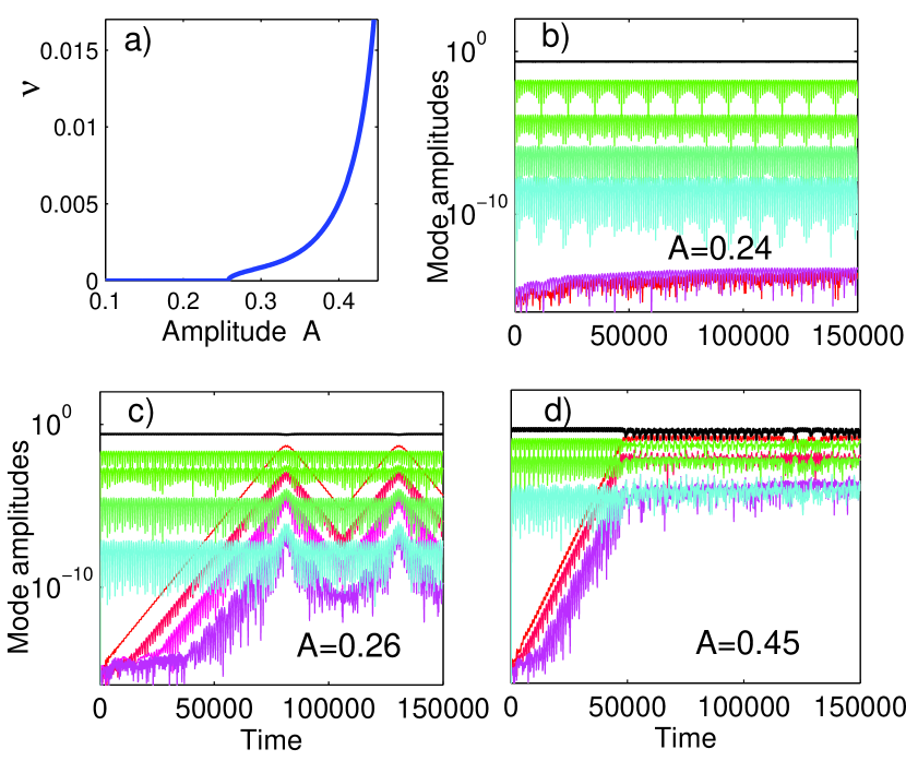
Figure 3: a) Analytically calculated growth rate according to formula (15) in the case of the short-range FPU model. b) and c) display mode stability/instability near the theoretically predicted threshold value. d) shows mode dynamics far from the instability threshold value. In all simulations, $N=32$.

Now it is straightforward to extend the study of this unusual instability behavior to the conventional short-range FPU model. Indeed, mode evolution, Eq. (5), is applicable for the short-range case as well, the only difference is contained in the unperturbed frequencies $\Omega_{n}^{0}$. Note that in the short-range FPU unperturbed frequencies of low modes are almost equidistant, see Fig. 1a., in contrast to the long-range case. Therefore, the denominator in Eq. (9) is close to zero, which is the reason for the well known phenomenon of FPU recurrences (large energy transfer between the low modes) FPU ; galavotti ; tod . Thus, although the instability mechanism is present in short-range as well, the energy exchange among modes does not allow steady exponential growth of the unexcited modes. The short-range FPU instability develops completely only for larger values of the amplitude $A$, when instabilities are not sporadic.

Seeking for the resonant modes in the short-range FPU model, one finds the set $n=2$, $m=N-2$, $r=1$, $p=3$ with frequencies $\Omega_{2}$, $\Omega_{2}$, $\Omega_{1}$, $3\Omega_{1}$, respectively. Then the condition $\Delta=0$ is reached for $A=0.29$. Plotting again the growth rate $\nu$ versus $A$ according to the formula (15), we get the dependence presented in Fig. 3a. The instability is no more sporadic: instead, after it is triggered at a given value of $A=0.249$, it persists for all larger values. In Figs. 3b-d, we plot the modes amplitude evolution for different values of $A$. Instability develops in the range $A=0.24-0.26$, in excellent agreement with theoretical predictions.

Finally, as concluding remarks, we address the question of estimating the threshold amplitude $A_{th}$ below which no sporadic instability takes place in the large $N$ limit. The total number of harmonics in the $N$ modes (see e.g. Eq. (9) for the third mode) scales as $N!\sim N^{N}$; consequently the distance between neighboring harmonics decreases as $N^{-N}$. Therefore, the average detuning $\Delta$ in formula (15) should be of the same order and thus $\Delta^{2}\sim N^{-2N}$. On the other hand, the first term under the square root scales as $(A_{th}^{2}/N^{4})^{N}$ in the perturbative limit. From the condition that the growth rate in Eq. (15) is real it follows that $A_{th}\sim N$ (this estimate is compatible with recent unpublished numerical experiments newexp ). Therefore, the energy density threshold remains finite at large $N$, $\epsilon_{th}=E_{th}/N\sim A_{th}^{2}/N^{2}\sim const.$.

- (1) Chaos, Focus Issue, 15 The ”Fermi-Pasta-Ulam” problem: the first fifty years (2005).
- (2) G. Gallavotti (Editor), The Fermi-Pasta-Ulam problem: a status report, Springer Verlag, Berlin (2008).
- (3) T. Dauxois, Physics Today 61, 55, (2008); T. Dauxois and S. Ruffo, Fermi-Pasta-Ulam nonlinear lattice oscillations, Scholarpedia, 3 (8), 5538 (2008).
- (4) A. Campa, T. Dauxois T. and S. Ruffo, Phys. Rep., 480, 57 (2009).
- (5) A. Campa, T. Dauxois, D. Fanelli and S. Ruffo, Physics of long-range interacting systems, Oxford University Press (2014).
- (6) S. Flach, Phys. Rev. E, 58, R4116 (1998); Physica D, 113, 184 (1998).
- (7) V.E. Tarasov, G.M. Zaslavsky, Commun. Nonlinear Sci. Numer. Simul., 11, 885 (2006).
- (8) H. Christodoulidi, C. Tsallis and T. Bountis, Europhys. Lett., 108, 40006 (2014).
- (9) Yu. B. Gaididei, S. F. Mingaleev, P. L. Christiansen, R. O. Rasmussen, Phys. Rev. E, 55, 6141 (1997); S. F. Mingaleev, P. L. Christiansen, Yu. B. Gaididei, M. Johansson, K. O. Rasmussen, J. Biol. Phys., 25, 41 (1999); J. Cuevas, F. Palmero, J. F. R. Archilla, F. R. Romero, Phys. Lett. A 299, 221 (2002).
- (10) A. Picinin, M.H. Lente, J.A. Eiras, J.P. Rino, Phys. Rev. B, 69, 064117 (2004).
- (11) Varon M. et al., Sci. Rep., 3 1234 (2013); M.R. Roser, L.R. Corruccini L. R., Phys. Rev. Lett., 65 1064 (1990).
- (12) G. Gori, T. Macry, A. Trombettoni, Phys. Rev. E, 87, 032905 (2013).
- (13) T. Lahaye, C. Menotti, L. Santos, M. Lewenstein and T. Pfau, Rep. Prog. Phys., 72, 126401 (2009).
- (14) R. Heidemann et al., Phys. Rev. Lett., 100, 033601 (2008); P. Schauss et al., Nature (London), 491, 87 (2012).
- (15) R. Bachelard and M. Kastner, Phys. Rev. Lett., 110, 170603 (2013); J. Eisert, M. van den Worm, S. Manmana and M. Kastner, Phys. Rev. Lett., 111, 260401 (2013).
- (16) P. Richerme et al., Nature (London), 511, 198 (2014); P. Jurcevic et al., Nature (London), 511, 202 (2014).
- (17) A. Picozzi, J. Garnier, T. Hansson, P. Suret, S. Randoux, G. Millot, D. N. Christodoulides, Phys. Rep., 541, 1 (2014).
- (18) L. Laurson et al., Nature Communications, 4, 2927, (2013); D. Bonamy, S. Santucci, L. Ponson, Phys. Rev. Lett. 101, 045501 (2008).
- (19) J.F. Joanny, P.G. De Gennes, J. Chem. Phys. 81, 552 562 (1984).
- (20) F. Fucito et al., Journ. de Physique (Paris), 43, 707 (1982).
- (21) S. Flach, M.V. Ivanchenko, O.I. Kanakov, Phys. Rev. Lett. 95, 064102 (2005) and Phys. Rev. E, 73, 036618 (2006).
- (22) C.F. Driscoll, T.M. O’Neil, Phys. Rev. Lett. 37, 69 (1976); C.F. Driscoll, T.M. O’Neil, Rocky Mt. J. Math. 5, 211 (1978).
- (23) P. Poggi and S. Ruffo, Physica D, 103, 251 (1997).
- (24) G.M. Chechin, N.V. Novikova, A.A. Abramenko, Physica D 166, 208 (2002).
- (25) H. Christodoulidi, C. Efthymiopoulos, Physica D, 261, 92 (2013).
- (26) N. Saito, N. Hirotomi, A. Ichimura, J. Phys. Soc. Jpn., 39, 1931 (1975); G. Christie, B.I. Henry, Phys. Rev. E, 58, 3045 (1998).
- (27) The second term in (2) is chosen in view of ensuring periodic boundary conditions and translational invariance of the model, which enables us to diagonalize the harmonic interaction in momentum space. This term vanishes in the thermodynamic limit and so has little relevance in analytical considerations but could have a significant impact on numerical simulations, where achieving this limit is impossible.
- (28) G. Chechin and S. Shcherbinin, private communication.