Statistical Survey of Type III Radio Bursts at Long Wavelengths Observed by the Solar TErrestrial RElations Observatory (STEREO)/Waves Instruments: Radio Flux Density Variations with Frequency
Abstract
We have performed a statistical study of Type III radio bursts observed by Solar TErrestrial RElations Observatory (STEREO)/Waves between May 2007 and February 2013. We have investigated the flux density between kHz and MHz. Both high- and low-frequency cutoffs have been observed in % of events suggesting an important role of propagation. As already reported by previous authors, we observed that the maximum flux density occurs at MHz on both spacecraft. We have developed a simplified analytical model of the flux density as a function of radial distance and compared it to the STEREO/Waves data.
keywords:
Solar radio emissions, Plasma radiation1 Introduction
S-intro
Type III radio bursts are consequence of suprathermal electrons accelerated during solar flares [Wild (1950)]. The Type III-generating electron beam propagates outward from the Sun along an open magnetic field line in the interplanetary (IP) medium with speed ranging from c to c [Dulk et al. (1987), Mel’nik, Lapshin, and Kontar (1999), Dulk (2000)]. As the electron beam produces the bump-on-tail instability, it locally excites intense Langmuir waves at the local electron plasma frequency []. These waves then convert to electromagnetic emission via a series of non-linear processes which are still debated and require better understanding [Melrose (1980), Robinson and Cairns (1998)].
The generation of Langmuir waves by the beam also produces back-reaction on the local distribution of electrons, which makes the problem of electron propagation inherently non-linear. The characteristic scales of electron-beam propagation ( AU) require additional simplifications such as quasi-linear treatment [Drummond and Pines (1962), Vedenov, Velikhov, and Sagdeev (1962), Pines and Schrieffer (1962)]. The relatively low level of the waves is normally justified by the observations of the mean electric fields associated with Type III exciters. The numerical simulations of transport and generation as well as re-absorption of Langmuir waves show that the electron beam can propagate over large distances with relatively weak losses while at the same time producing a high level of plasma waves locally [Magelssen and Smith (1977)]. The important aspect of beam–Langmuir wave evolution is the sensitivity to plasma–density fluctuations in the solar corona and the heliosphere. The density fluctuations can effectively influence the distribution of waves, which in turn affects the electron distribution [Smith and Sime (1979), Melrose, Cairns, and Dulk (1986)]. Numerical simulations [Kontar (2001)] also reveal that the plasma inhomogeneities change the spatial distribution of the waves, while the local electron distribution is weakly affected. However, the effects of density fluctuations and large–scale density gradient in the solar plasma becomes noticeable at large distances [Kontar and Reid (2009)], so that initially injected power-law spectrum becomes a broken one. Overall, the rate at which plasma waves are induced by an unstable electron beam is reduced by background density fluctuations, most acutely when fluctuations have large amplitudes or small wavelengths. Numerical simulations [Reid and Kontar (2010)] further show a direct correlation between the spectrum of the double power-law below the break energy and the turbulent intensity of the background plasma.
Langmuir waves can be converted via the plasma emission process [Ginzburg and Zhelezniakov (1958)] into electromagnetic radiation: Type III radio bursts either at [the fundamental [F] component], and/or at [the harmonic [H] component]. Although this mechanism has been extensively investigated, the conversion itself still remains under debate. Type III radio bursts can be observed from metric to kilometric wavelengths [Reiner et al. (2000)]. From metric to decametric wavelengths we can usually distinguish the F- and H-components while the F-component is often more intense than the H-component. At kilometric wavelengths it is problematic to determine the observed component. \inlinecite1980ApJ…236..696K has developed a method for determination of the component for cases when Type III triggering electron beams intersect the spacecraft.
Propagation of Type III radio bursts from the source to the spacecraft is affected both by refraction in density gradients and scattering by inhomogeneities in the solar wind ranging on all scales from km to AU. These effects result in the shifted position of a source location, enlargement of the source size, and decrease of the flux density and degree of polarization [Dulk (2000)]. Better understanding of proper images of radio sources may shed light on physical processes along the path of the exciter electrons in the IP medium.
While previous solar spacecraft used for Type III radio-burst investigation were all spin-stabilized (International Sun/Earth Explorer 3, Ulysses, Wind, etc.), Solar TErrestrial RElations Observatory (STEREO; \opencite2008SSRv..136….5K) is the first three-axis stabilized solar mission to observe these waves. With the two identical STEREO spacecraft and their suite of state-of-the-art instruments, we can study mechanisms and sites of solar energetic-particle acceleration in the low corona and the IP medium. The STEREO/Waves instrument enables us to measure radio flux density from decametric to kilometric wavelengths. Therefore we can investigate global distributions of radio sources in the solar wind when an appropriate electron-density model is used.
In this article, we present statistical results on the frequency spectra of Type III radio bursts at long (i.e. from dekametric to kilometric) wavelengths observed by STEREO/Waves. This is the first of two linked articles that summarize our findings on statistical properties of Type III radio bursts. In this article we focus on a flux density and its relation to electron beams producing these bursts. Goniopolarimetric (GP; also referred to as direction-finding) results will be discussed in the second article [Krupar et al. (2014)].
In Section \irefS-data we describe the instrumentation and data processing. In Section \irefS-Results we analyze two Type III radio bursts and describe our statistical data set. Next we present a statistical examination of Type III radio bursts with focus on the frequency spectra and the model of the flux density as a function of the radial distance. In Section \irefS-Conclusion we summarize our findings and we make concluding remarks.
2 Instrumentation and Methodology
S-data
2.1 The STEREO/Waves Instrument
S-stereo
STEREO provides us with first stereoscopic measurements of the solar phenomena using identical instruments onboard [Biesecker, Webb, and St. Cyr (2008)]. The two STEREO spacecraft are three-axis stabilized and carry the STEREO/Waves instruments, which measure electric-field fluctuations between 2.5 kHz and 32.025 MHz [Bougeret et al. (2008), Bale et al. (2008)]. The three monopole antenna elements (six meters long), made from beryllium–copper, are used by STEREO/Waves to measure electric-field fluctuations [Bale et al. (2008)]. Although we use three orthogonal antennas, their effective antenna directions [ and ] and lengths [] are different from the physical ones due to their electrical coupling with the spacecraft body.
For our survey we have used data from the High Frequency Receiver (HFR: a part of the STEREO/Waves instrument; \opencite2008SSRv..136..487B), which is a dual-channel receiver (connected to two antennas at one time) operating in the frequency range kHz – MHz with a kHz effective bandwidth. HFR has instantaneous GP capabilities between kHz and kHz allowing us to retrieve the direction of arrival of an incoming electromagnetic wave, its flux, and its polarization properties [Cecconi et al. (2008)]. HFR consists of two receivers: HFR1 ( kHz – kHz, frequency channels) and HFR2 ( kHz – MHz, frequency channels). HFR1 provides us with auto- and cross-correlations on all antennas (three monopoles), while HFR2 has retrieved only two auto-correlations (one monopole and one dipole) for most of the time since May 2007.
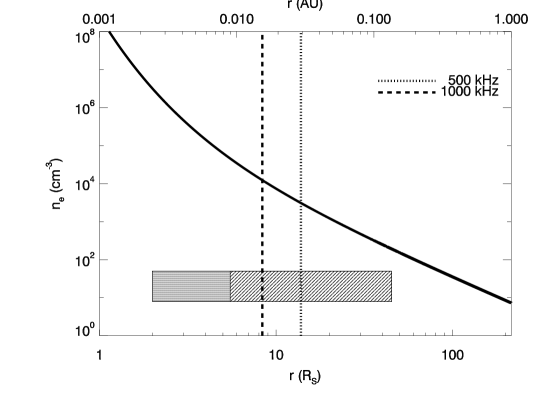
Using a semiempirical model of electron density [] in the solar corona and IP medium [Sittler and Guhathakurta (1999)] we can assign particular frequencies to radial distances from the Sun. Consequently STEREO/Waves/HFR allows us to investigate GP properties of radio sources located between and while the intensity is measured up to above the Sun’s surface (Figure \irefsittler).
For converting the voltage power spectral density at the terminals of the antennas [: ] into physical units we have applied the method described by \inlinecite2011RaSc…46.2008Z. In order to compute the flux density [: ] as below, we need to know the effective antenna lengths and receiver properties.
| (1) |
| (2) |
where denotes the impedance of vacuum. The -coefficient is the gain factor of the receiver-antenna system and is composed from the antenna capacitance [] and the stray capacitance [].
The model of the galactic background brightness [], as a nearly stable isotropic source, allows us to determine reduced effective antenna lengths [] according to \inlinecite2011RaSc…46.2008Z:
| (3) |
| (4) |
| (5) |
where and is the frequency in MHz [Novaco and Brown (1978)]. The represents a square noise generated by the receiver itself and hence should be subtracted before the antenna calibration. We have adapted values from \inlinecite2011RaSc…46.2008Z:
-
•
dB for STEREO-A channel1
-
•
dB for STEREO-A channel2
-
•
dB for STEREO-B channel1
-
•
dB for STEREO-B channel2
These values have been obtained by -minimization considering the to be frequency independent [Zaslavsky et al. (2011)]. We have performed the same analysis as \inlinecite2011RaSc…46.2008Z in order to obtain accurate reduced effective antenna lengths [] as a function of frequency (Figure \irefsta31). These parameters have been retrieved by comparing the lowest % of the data observed within one day (13 January 2007) and the modeled galactic background [] using the Equation (\irefeq:gammaleff). The low frequency part [ kHz] is mostly affected by the shot noise induced by solar-wind particles impacting on the antennas [Bougeret et al. (2008)] and by the quasi-thermal noise (QTN) produced by the ambient plasma [Meyer-Vernet and Perche (1989)]. Since these effects are stronger than the galactic background, the method used is not reliable for retrieving for the low frequency part.
On the other hand, the short dipole approximation for STEREO antennas is not valid for frequencies above MHz since corresponding wavelengths become comparable with the reduced effective antenna length [] and thus induced voltages are not proportional to electric field fluctuations [Bale et al. (2008)]. In Figure \irefsta31 we can identify several frequency channels (24 for STEREO-A and 26 for STEREO-B from a total of 319, i.e. %) with larger than their neighboring frequency channels. When the measured signal is significantly larger than the fit of the galactic background model, it is likely that this discrepancy is due to instrumental effects, e.g. frequency interferences [Zaslavsky et al. (2011)]. We have excluded these outlying values of from our analysis.
For HFR1 ( MHz) we have used fixed reduced antenna effective lengths (e.g. see dashed lines in Figure \irefsta31 for the Z antennas). Measured fluxes by the three monopoles have been transformed into the orthogonal frame using effective antenna directions obtained by observations of the non-thermal Auroral Kilometric Radiation (AKR) during STEREO-B roll maneuvers [Krupar et al. (2012)]. As no AKR has been observed by STEREO-A, the effective directions have been assumed to be the same. The three calculated orthogonal components of the flux density are summed to obtain the total flux density induced by an incident radio wave.
The antenna calibration for HFR2 ( MHz) is more complex, as two effects play a part, resulting in the reduced antenna effective length being larger than the physical one for higher frequencies above MHz [Zaslavsky et al. (2011)]. The first effect is the half-wave resonance that changes the effective antenna formulas to be functions of frequency. The second one is the increase of above one due to the electrical-circuit resonance as the antenna becomes inductive (). Above MHz the reduced effective antenna length rapidly changes and the conversion to physical units according to Equation (\irefeq:s) becomes inaccurate. For HFR2 we have used reduced antenna effective lengths from Figure \irefsta31 as a function of frequency. We have summed both contributions of the X–Y dipole and the Z-monopole to obtain the total flux density.
In order to improve the signal-to-noise ratio we have subtracted receiver background levels from the data before we performed our analysis. These levels have been calculated as the median values over a period of 15 days (7 before, the corresponding one, and 7 after) of the given auto-correlation for each channel–antenna configuration separately.
3 Results and Discussion
S-Results
We have manually selected 152 time–frequency intervals when Type III radio bursts have been observed by STEREO/Waves between May 2007 and February 2013. The separation angle between spacecraft in the ecliptic plane ranged between (May 2007) and (February 2011). We have included only simple and isolated events when flux density was intense enough for the GP analysis.
3.1 6 May 2009 Type III Radio Burst
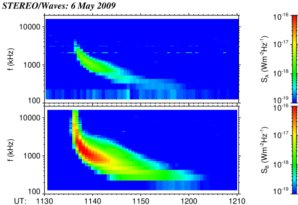
S-event1 As an example from our list of events we present a Type III radio burst observed on 6 May 2009 by both STEREO spacecraft (Figure \iref20090506_psd). A faint A3.8 X-ray flare located at NE triggered the Type III radio burst. During this event STEREO-A was at West from the Sun–Earth line at AU from the Sun whereas STEREO-B was located at East and AU from the Sun. The separation angle between the STEREO spacecraft in the ecliptic plane was . STEREO-B, located near the source by longitude, observed the Type III radio burst to have been much intense than STEREO-A being at longitude from the source. Also the spectral shape of the emission at STEREO-B is much broader than at STEREO-A. The onset time of the Type III radio burst was observed about one minute earlier at STEREO-B than at STEREO-A. Whilst the frequency cutoff was not observed at STEREO-B, the radio burst is detected between kHz and MHz only at STEREO-A.
As we do not observe the triggering electron beam, we are unable to use the method of \inlinecite1980ApJ…236..696K to distinguish the F- and H-components of the Type III radio burst. When both components are observed, the F-component has typically larger flux density than the H-component [Dulk et al. (1998)]. Using Monte Carlo simulations, \inlinecite2007ApJ…671..894T showed that scattering due to random density fluctuations at kHz extends the visibility of the F-and H-components from to and from to , respectively. In other words, the F-component is visible only in a narrow cone from a source only when compared to H-component being visible almost everywhere. From spectral shapes and relative positions between the spacecraft and the flare site, we may conclude that STEREO-B most probably observed the F- and H-components whereas STEREO-A measured the H-component only.
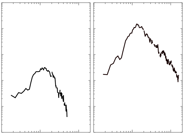
Figure \iref20090506_ls displays peak fluxes as a function of frequency for STEREO-A (on the left) and STEREO-B (on the right). A signal detected at STEREO-B is about larger than at STEREO-A. It is in agreement with position of the solar flare site, detected a lower signal at STEREO-A (Figure \iref20090506_ls), and an observed difference of onset times between the two spacecraft (Figure \iref20090506_psd). The maximum flux density at both spacecraft occurs at MHz.
We may identify a discontinuity in the HFR1/HFR2 connection at MHz on STEREO-A but not on STEREO-B.
3.2 23 November 2011 Type III Radio Burst
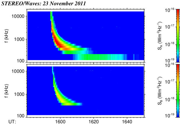
S-event2 As another example we present a Type III radio burst observed on 23 November 2011 by the two STEREO spacecraft. STEREO-A was at West from the Sun–Earth line at AU from the Sun while STEREO-B was located East at AU from the Sun. The separation angle between the STEREO spacecraft in the ecliptic plane was . Figure \iref20111123_psd shows flux density [] from STEREO-A and STEREO-B when an intense Type III radio burst was detected at around 15:55 UT. We have not linked this event to any solar flare as the active region was probably located on the far side of the Sun from the Earth’s perspective. The radio burst covers the full frequency range at STEREO-A. STEREO-B observed the emission above kHz.
Figure \iref20111123_ls displays peak fluxes as a function of frequency for STEREO-A (on the left) and STEREO-B (on the right). A signal detected at STEREO-A is about ten times larger than at STEREO-B. The maximum flux density occured at kHz. We observed increase of the flux above MHz at both spacecraft. This increase can be caused by the antenna calibration when we are close to the half wave resonance. Moreover, some additional calibration effects may take place here. We have decided to keep such events in our data set since this flux increase might be a real feature of Type III radio bursts.
We do not identify any discontinuity in the HFR1/HFR2 connection at MHz, which suggests that we can combine measurements of the monopole mode (HFR1) with the dipole/monopole mode (HFR2).
3.3 Data Set
S-time
Table \ireftab:stat summarizes Type III radio bursts included in our statistical survey. Numbers of events from both spacecraft are about the same. For the reasons described in Section 3.1 we do not distinguish F/H components at long wavelengths in our data set. Generally, the F component is more intense and more directive when compared to the H component [Dulk (2000), Thejappa, MacDowall, and Kaiser (2007)]. These two opposing effects cause uncertainty which of the two components is predominant in our data set. Therefore, we will discuss our results considering that both plasma emission processes take place.
The topmost panel of Figure \irefhisto_events displays the histogram of the observed Type III radio bursts vs time at STEREO-A and STEREO-B. The middle panel is the separation angle between STEREO-A and STEREO-B. The last panel contains absolute measurements of flux density from the Sun at a wavelength of 10.7 centimeters averaged over the month measured on the ground (www.spaceweather.gc.ca). This value can be used as an estimator of the solar activity. Although the Sun exhibited increased activity as of 2011 we do not have many events from this period since we include only simple and isolated emissions.
We have compared onset times of Type III radio bursts with onset times of solar flares listed by the Lockheed Martin Solar and Astrophysics Laboratory (www.lmsal.com/solarsoft/latest_events_archive.html). We have been able to link only bursts with solar flares (from total of 152, i.e. % of all events). Since X-ray imagers are located close to the Earth, we have more linked events in 2007 (up to %, when the two STEREO were near the Earth) compared to 2012 – 2013 when only few Type III radio bursts have been associated (the two STEREO spacecraft were on the far side of the Sun).
Figure \irefflare_histo shows a histogram of solar flares responsible for the aforementioned 31 Type III radio bursts (flare class A: 6 events, flare class B: 15 events, flare class C: 9 events, flare class M: 1 event). Generally, more intense solar flares trigger complex Type III radio bursts which are not the area of our interest.
We have also compared events from our data set with ground-based observations. The results will be addressed in a separate publication.
3.4 Frequency Distribution
S-frq Figure \ireffrq_dist displays histograms of frequencies of all Type III radio bursts from our data set for STEREO-A (solid line) and STEREO-B (dotted line). When combined with the number of events (Table 1) it demonstrates the number of data points used in our survey. Although at STEREO is typically around kHz, only % (STEREO-A) and % (STEREO-B) of events have been measured up to kHz corresponding to the lowest-frequency channel of HFR. Our statistical results on low-frequency cutoffs are generally comparable with previous studies dedicated to Wind and Ulysses observations, e.g. by \inlinecite1996A&A…316..406L and \inlinecite1996GeoRL..23.1203D. \inlinecite1995GeoRL..22.3429L suggest that the low-frequency cutoff can be explained as i) an intrinsic characteristic of the radiation mechanism, ii) an effect of a directivity of the radiation, and iii) propagation effects between the source and the observer.
On the other hand more than % of Type III radio bursts are observed up to MHz, which corresponds to a source position located and above the Sun’s surface assuming the F- and H-emission, respectively (Figure \irefsittler). Concerning high-frequency cutoffs, \inlinecite2000GMS…119..115D investigated events observed by the Wind spacecraft and % of them started at frequencies below MHz – the maximum frequency recorded by the instrument. In our dataset we have around % of radio bursts that commence at frequencies below MHz.
3.5 Statistical Analysis of the Frequency Spectra
S-stat
We have identified frequencies corresponding to the maximum-flux density for each Type III radio burst separately. Table \ireftab:max_frq contains statistical distributions of these peak frequencies. Medians of peak frequencies are around MHz ( kHz at STEREO-A and kHz at STEREO-A) which is in agreement with previous observations. \inlinecite1978SoPh…59..377W found in data from the Interplanetary Monitoring Platform-H (IMP-6) spacecraft ( kHz) that the maximum flux density occurs at MHz.
We have investigated median values of the flux density vs. frequency (see Figure \irefint1). As the distribution has a log-normal character, we have used median values instead of mean ones. The maximum flux density ( or sfu) occurs at MHz on both spacecraft. The low-frequency part is affected by the QTN and shot noise, especially for STEREO-A. We have observed a slight increase of flux at STEREO-A for frequencies above MHz but not at STEREO-B. In the case of STEREO-B, it is covered by noise as the th percentile exhibits the same trend (Figures \iref20090506_ls and \iref20111123_ls). This increase can be caused by inconsistencies of the antenna calibration when we are close to the half-wave resonance (Figure \irefsta31). On the other hand it can be a real feature of Type III radio bursts. Unfortunately, we cannot compare our results with previous studies since this frequency range ( MHz — MHz) has not been investigated by space-borne nor ground-based instruments. Therefore we conclude that measurements of frequencies above MHz should be considered carefully.
3.6 Interpretation of the MHz maximum
S-model
Using the electron-density model of the solar wind we can determine average distances of radio sources from the Sun of Type III radio bursts (Figure \irefsittler). A frequency of MHz corresponds to a radio source located at and from the Sun for the F- and H-component, respectively (dashed and dotted lines in Figure \irefsittler). The plasma density [] in the corona decreases faster than , but starting from around it decreases as (a solid line in Figure \irefsittler). The MHz maximum in Figure \irefint1 coincides with this region. One should note that the critical radius of Parker’s model of the solar-wind expansion is typically about being roughly between and .
We have developed a simplified analytical model of the flux density as a function of radial distance. Let us consider propagation and generation of plasma waves in the corona. Assuming fast relaxation of the beam, we find that the beam propagates as a beam-plasma structure (e.g. \opencite2001A&A…375..629K), so that the 1D electron distribution function [] is
| (6) | |||||
and the spectral energy density of Langmuir waves with wavenumber is
| (7) |
where is the plateau-like electron distribution function of the beam electrons, their number density, is the maximum velocity of the plateau electrons, is electron mass, and is the 1D Langmuir-Waves spectral density. Let us first consider emission at the spatial peak, e.g. and near the spectral peak :
| (8) |
In a case where of the H-component of an electromagnetic (EM) radiation is saturated we consider its spectral energy density [] to be proportional to the energy of Langmuir waves [Melrose (1980)]:
| (9) |
The spectral flux density of the H-component at the Earth [] can be estimated (the same as if the spacecraft is at AU):
| (10) |
where , is the group velocity of the EM waves, is the area of the source, and is the AU distance. Hence one finds, ignoring constants:
| (11) |
where is the plasma frequency. Further assuming that , one obtains
| (12) |
We have included the model in arbitrary units in Figure \irefint1. The semiempirical model of electron density of \inlinecite1999ApJ…523..812S in the solar corona and IP medium has been used for estimating . The model of the flux density as a function of frequency [] exhibits a maximum at MHz (corresponding to a radio source located at from the Sun’s center) that differs from the observation (maximum at MHz). The model assumes the H-emission only since a relation between the spectral energy density for the F-emission and the energy of Langmuir waves [] is not obvious.
However, we have modified the model for the F-component considering that the radio flux is proportional between the two components []. In this case we have obtained a maximum at MHz being in a better agreement with the observed maximum at MHz. One should note that this approach is very simplified omitting many physical processes such as an efficiency of Langmuir and radio waves conversion, volume of source regions, and scattering of radio beams by density fluctuations.
4 Summary and Concluding Remarks
S-Conclusion Type III radio bursts belong among the most intense electromagnetic emissions in the heliosphere. They can be observed from tens of kHz up to several GHz. They are frequently detected by STEREO/Waves instruments, which provide us with a unique stereoscopic view of radio sources in a frequency range from kHz to MHz. These frequencies correspond to radial distances from the Sun from to and to for the F- and H-component, respectively.
We have investigated properties of simple and isolated Type III radio bursts observed by the two STEREO spacecraft between May 2007 and February 2013. We show a detailed analysis of two events from our data set, as an example.
Our main statistical results on the frequency spectra are as follows:
-
i)
We have observed the low-frequency cutoff at kHz in % — % of events.
-
ii)
More than % of Type III radio bursts are observed up to MHz, which corresponds to a source position located R⊙ and R⊙ from the Sun’s surface for the F- and H-component, respectively.
-
iii)
We have found that the maximum of flux density ( ) occurs at MHz on both spacecraft which corresponds to radio sources located at and for the F- and H-component, respectively.
-
iv)
We have introduced a simple model of the radio emission flux density vs. radial distance which provides us with a peak at a frequency within a factor of four (the H-component) and two (the F-component) from the observation, respectively.
The observed low- high-frequency cutoffs can be explained by intrinsic features of radio sources, their directivity, and/or propagation effects between the source and the spacecraft. The source region of radio emissions at MHz corresponds to the region where a change of the plasma density gradient takes place.
We have also observed an increase of the flux density above MHz, which corresponds to radial distances from the Sun of and for the F- and H-component, respectively. We conclude that results of the radio flux above MHz are questionable probably due to instrumental effects.
The model for the H-component exhibits a peak at MHz. We have modified the model for the F-component and the obtained maximum at MHz better corresponds to the maximum observed in the data. One should note that various assumptions on an electron density profile in the solar wind, variations of an exciter speed, and an electron beam density profile may lead to different maximum locations.
In the future we plan to perform simulations of the resonant interaction of an electron beam with Langmuir waves in connection with the observed MHz maximum.
Acknowledgements
S-ack The authors would like to thank the many individuals and institutions who contributed to making STEREO/Waves possible. J. Soucek acknowledges the support of the Czech Grant Agency grant GAP209/12/2394. O. Kruparova thanks the support of the Czech Grant Agency grant GP13-37174P. Financial support by STFC and by the European Commission through the ”Radiosun” (PEOPLE-2011-IRSES-295272) is gratefully acknowledged (E.P. Kontar). O. Santolik and V. Krupar acknowledge the support of the Czech Grant Agency grant GAP205/10/2279.
| STEREO-A events | 135 |
| STEREO-B events | 127 |
| STEREO-A and STEREO-B | 110 |
| STEREO-A and not STEREO-B | 25 |
| STEREO-B and not STEREO-A | 17 |
| Total number of events | 152 |
| STEREO-A | STEREO-B | |
|---|---|---|
| Mean [kHz] | 1291 | 1498 |
| STD [kHz] | 1534 | 1894 |
| Median [kHz] | 825 | 925 |
| th percentile [kHz] | 525 | 625 |
| th percentile [kHz] | 1575 | 1875 |


References
- Bale et al. (2008) Bale, S.D., Ullrich, R., Goetz, K., Alster, N., Cecconi, B., Dekkali, M., Lingner, N.R., Macher, W., Manning, R.E., McCauley, J., Monson, S.J., Oswald, T.H., Pulupa, M.: 2008, The Electric Antennas for the STEREO/WAVES Experiment. Space Sci. Rev. 136, 529. DOI. ADS.
- Biesecker, Webb, and St. Cyr (2008) Biesecker, D.A., Webb, D.F., St. Cyr, O.C.: 2008, STEREO Space Weather and the Space Weather Beacon. Space Sci. Rev. 136, 45. DOI. ADS.
- Bougeret et al. (2008) Bougeret, J.L., Goetz, K., Kaiser, M.L., Bale, S.D., Kellogg, P.J., Maksimovic, M., Monge, N., Monson, S.J., Astier, P.L., Davy, S., Dekkali, M., Hinze, J.J., Manning, R.E., Aguilar-Rodriguez, E., Bonnin, X., Briand, C., Cairns, I.H., Cattell, C.A., Cecconi, B., Eastwood, J., Ergun, R.E., Fainberg, J., Hoang, S., Huttunen, K.E.J., Krucker, S., Lecacheux, A., MacDowall, R.J., Macher, W., Mangeney, A., Meetre, C.A., Moussas, X., Nguyen, Q.N., Oswald, T.H., Pulupa, M., Reiner, M.J., Robinson, P.A., Rucker, H., Salem, C., Santolik, O., Silvis, J.M., Ullrich, R., Zarka, P., Zouganelis, I.: 2008, S/WAVES: The Radio and Plasma Wave Investigation on the STEREO Mission. Space Sci. Rev. 136, 487. DOI. ADS.
- Cecconi et al. (2008) Cecconi, B., Bonnin, X., Hoang, S., Maksimovic, M., Bale, S.D., Bougeret, J.-L., Goetz, K., Lecacheux, A., Reiner, M.J., Rucker, H.O., Zarka, P.: 2008, STEREO/Waves Goniopolarimetry. Space Sci. Rev. 136, 549. DOI. ADS.
- Drummond and Pines (1962) Drummond, W., Pines, D.: 1962, Non-Linear Stability of Plasma Oscillations. Nuclear Fusion 3, 1049.
- Dulk (2000) Dulk, G.A.: 2000, Type III Solar Radio Bursts at Long Wavelengths. Geophys. Mono. Ser., AGU 119, 115. ADS.
- Dulk et al. (1987) Dulk, G.A., Goldman, M.V., Steinberg, J.L., Hoang, S.: 1987, The speeds of electrons that excite solar radio bursts of type III. A&A 173, 366. ADS.
- Dulk et al. (1996) Dulk, G.A., Leblanc, Y., Bougeret, J.-L., Hoang, S.: 1996, Type III bursts observed simultaneously by Wind and Ulysses. Geophys. Res. Lett. 23, 1203. DOI. ADS.
- Dulk et al. (1998) Dulk, G.A., Leblanc, Y., Robinson, P.A., Bougeret, J.-L., Lin, R.P.: 1998, Electron beams and radio waves of solar type III bursts. J. Geophys. Res. 103, 17223. DOI. ADS.
- Ginzburg and Zhelezniakov (1958) Ginzburg, V.L., Zhelezniakov, V.V.: 1958, On the Possible Mechanisms of Sporadic Solar Radio Emission (Radiation in an Isotropic Plasma). Soviet Ast. 2, 653. ADS.
- Kaiser et al. (2008) Kaiser, M.L., Kucera, T.A., Davila, J.M., St. Cyr, O.C., Guhathakurta, M., Christian, E.: 2008, The STEREO Mission: An Introduction. Space Sci. Rev. 136, 5. DOI. ADS.
- Kellogg (1980) Kellogg, P.J.: 1980, Fundamental emission in three type III solar bursts. ApJ 236, 696. DOI. ADS.
- Kontar (2001) Kontar, E.P.: 2001, Dynamics of electron beams in the solar corona plasma with density fluctuations. A&A 375, 629. DOI. ADS.
- Kontar and Reid (2009) Kontar, E.P., Reid, H.A.S.: 2009, Onsets and Spectra of Impulsive Solar Energetic Electron Events Observed Near the Earth. ApJ 695, L140. DOI. ADS.
- Krupar et al. (2012) Krupar, V., Santolik, O., Cecconi, B., Maksimovic, M., Bonnin, X., Panchenko, M., Zaslavsky, A.: 2012, Goniopolarimetric inversion using SVD: An application to type III radio bursts observed by STEREO. J. Geophys. Res. 117(16), 6101. DOI. ADS.
- Krupar et al. (2014) Krupar, V., Maksimovic, M., Santolik, O., Cecconi, B., Kruparova, O.: 2014, Statistical Survey of Type III Radio Bursts at Long Wavelengths Observed by the Solar TErrestrial RElations Observatory (STEREO)/Waves Instruments: Goniopolarimetric Properties and Radio Source Locations, Solar Phys., submitted.
- Leblanc, Dulk, and Hoang (1995) Leblanc, Y., Dulk, G.A., Hoang, S.: 1995, The low radio frequency limit of solar type III bursts: Ulysses observations in and out of the ecliptic. Geophys. Res. Lett. 22, 3429. DOI. ADS.
- Leblanc et al. (1996) Leblanc, Y., Dulk, G.A., Hoang, S., Bougeret, J.-L., Robinson, P.A.: 1996, Type III radio bursts observed by ULYSSES pole to pole, and simultaneously by wind. A&A 316, 406. ADS.
- Magelssen and Smith (1977) Magelssen, G.R., Smith, D.F.: 1977, Nonrelativistic electron stream propagation in the solar atmosphere and type III radio bursts. Sol. Phys. 55, 211. DOI. ADS.
- Mel’nik, Lapshin, and Kontar (1999) Mel’nik, V.N., Lapshin, V., Kontar, E.: 1999, Propagation of a Monoenergetic Electron Beam in the Solar Corona. Sol. Phys. 184, 353. ADS.
- Melrose (1980) Melrose, D.B.: 1980, The emission mechanisms for solar radio bursts. Space Sci. Rev. 26, 3. DOI. ADS.
- Melrose, Cairns, and Dulk (1986) Melrose, D.B., Cairns, I.H., Dulk, G.A.: 1986, Clumpy Langmuir waves in type III solar radio bursts. A&A 163, 229. ADS.
- Meyer-Vernet and Perche (1989) Meyer-Vernet, N., Perche, C.: 1989, Tool kit for antennae and thermal noise near the plasma frequency. J. Geophys. Res. 94, 2405. DOI. ADS.
- Novaco and Brown (1978) Novaco, J.C., Brown, L.W.: 1978, Nonthermal galactic emission below 10 megahertz. ApJ 221, 114. DOI. ADS.
- Pines and Schrieffer (1962) Pines, D., Schrieffer, J.R.: 1962, Approach to Equilibrium of Electrons, Plasmons, and Phonons in Quantum and Classical Plasmas. Phys. Rev. E 125, 804. DOI. ADS.
- Reid and Kontar (2010) Reid, H.A.S., Kontar, E.P.: 2010, Solar Wind Density Turbulence and Solar Flare Electron Transport from the Sun to the Earth. ApJ 721, 864. DOI. ADS.
- Reiner et al. (2000) Reiner, M.J., Karlický, M., Jiřička, K., Aurass, H., Mann, G., Kaiser, M.L.: 2000, On the Solar Origin of Complex Type III-like Radio Bursts Observed at and below 1 MHZ. ApJ 530, 1049. DOI. ADS.
- Robinson and Cairns (1998) Robinson, P.A., Cairns, I.H.: 1998, Fundamental and Harmonic Emission in Type III Solar Radio Bursts - III. Heliocentric Variation of Interplanetary Beam and Source Parameters. Sol. Phys. 181, 429. DOI. ADS.
- Sittler and Guhathakurta (1999) Sittler, E.C. Jr., Guhathakurta, M.: 1999, Semiempirical Two-dimensional MagnetoHydrodynamic Model of the Solar Corona and Interplanetary Medium. ApJ 523, 812. DOI. ADS.
- Smith and Sime (1979) Smith, D.F., Sime, D.: 1979, Origin of plasma-wave clumping in type III solar radio burst sources. ApJ 233, 998. DOI. ADS.
- Thejappa, MacDowall, and Kaiser (2007) Thejappa, G., MacDowall, R.J., Kaiser, M.L.: 2007, Monte Carlo Simulation of Directivity of Interplanetary Radio Bursts. ApJ 671, 894. DOI. ADS.
- Vedenov, Velikhov, and Sagdeev (1962) Vedenov, A., Velikhov, E., Sagdeev, R.: 1962, Quasi-Linear Theory of Plasma Oscillations. Nuc. Fus., 465.
- Weber (1978) Weber, R.R.: 1978, Low frequency spectra of type III solar radio bursts. Sol. Phys. 59, 377. DOI. ADS.
- Wild (1950) Wild, J.P.: 1950, Observations of the Spectrum of High-Intensity Solar Radiation at Metre Wavelengths. III. Isolated Bursts. Austral. J. Sci. Res. A Phys. Sci. 3, 541. ADS.
- Zaslavsky et al. (2011) Zaslavsky, A., Meyer-Vernet, N., Hoang, S., Maksimovic, M., Bale, S.D.: 2011, On the antenna calibration of space radio instruments using the galactic background: General formulas and application to STEREO/WAVES. Radio Sci. 46, RS2008. DOI. ADS.