TTP14-028

An SU(5)$\,\times\,$A₅ Golden Ratio Flavour Model

Julia Gehrlein , Jens P. Oppermann , Daniela Schäfer , Martin Spinrath

Institut für Theoretische Teilchenphysik, Karlsruhe Institute of Technology,

Engesserstraße 7, D-76131 Karlsruhe, Germany

In this paper we study an SU(5)$\,\times\,$A₅ flavour model which exhibits a neutrino mass sum rule and golden ratio mixing in the neutrino sector which is corrected from the charged lepton Yukawa couplings. We give the full renormalisable superpotential for the model which breaks SU(5) and A₅ after integrating out heavy messenger fields and minimising the scalar potential. The mass sum rule allows for both mass orderings but we will show that inverted ordering is not valid in this setup. For normal ordering we find the lightest neutrino to have a mass of about 10-50 meV, and all leptonic mixing angles in agreement with experiment.

1 Introduction

Experimental results in the lepton sector have shed some new light on the origin of flavour. In contrast to the quark sector, lepton mixing angles have the distinctive feature that the atmospheric angle $\theta_{23}^{\text{PMNS}}$ and the solar angle $\theta_{12}^{\text{PMNS}}$, are both rather large [1]. Direct evidence for the reactor angle $\theta_{13}^{\text{PMNS}}$ was first provided by T2K, MINOS and Double Chooz [4, 2, 3]. Subsequently Daya Bay [5], RENO [6], and Double Chooz [7] Collaborations have measured $\sin^{2}(2\theta_{13}^{\text{PMNS}})$ to a high precision, see also Tab. 1.

Parameter	best-fit ($\pm 1\sigma$)	$3\sigma$ range
$\theta_{12}^{\text{PMNS}}$ in ∘	$33.48^{+0.77}_{-0.74}$	$31.30\rightarrow 35.90$
$\theta_{13}^{\text{PMNS}}$ in ∘	$8.52^{+0.20}_{-0.21}$	$7.87\rightarrow 9.11$
$\theta_{23}^{\text{PMNS}}$ in ∘	$42.2^{+0.1}_{-0.1}\oplus 49.4^{+1.6}_{-2.0}$	$38.4\rightarrow 53.3$
$\delta_{\text{PMNS}}$ in ∘	$251^{+67}_{-59}$	$0\rightarrow 360$
$\Delta m_{21}^{2}$ in $10^{-5}$ eV2	$7.50^{+0.19}_{-0.17}$	$7.03\rightarrow 8.09$
$\Delta m_{31}^{2}$ in $10^{-3}$ eV2 (NH)	$2.458^{+0.002}_{-0.002}$	$2.325\rightarrow 2.599$
$\Delta m_{32}^{2}$ in $10^{-3}$ eV2 (IH)	$-2.448^{+0.047}_{-0.047}$	$-2.590\rightarrow-2.307$

Table 1: The best-fit values and the 3$\sigma$ ranges for the parameters taken from [8]. There are two minima for $\theta_{23}^{\text{PMNS}}$. The first one corresponds to the normal hierarchy whereas the second one corresponds to the inverted hierarchy.

Among the many proposals trying to address the mixing patterns we will focus here on models exhibiting the so-called golden ratio (GR) mixing, where $\theta_{12}^{\text{PMNS}}$ is connected to the golden ratio $\phi_{g}=\tfrac{1+\sqrt{5}}{2}$.

A possible connection was first mentioned as a footnote in [9] and afterwards implemented in two different types of golden ratio models. In [9, 12, 10, 13, 11, 14] they find the prediction $\theta_{12}^{\text{PMNS}}=\tan^{-1}\left(\tfrac{1}{\phi_{g}}\right)\approx 31.7^{\circ}$ (golden ratio type A) to leading order while in [17, 15, 16, 14] they found $\theta_{12}^{\text{PMNS}}=\cos^{-1}(\phi_{g}/2)=36^{\circ}$ (golden ratio type B). More details on the history can be found as well in the excellent introduction of [13]. In this work we will find the first relation to leading order.

The neutrino mixing matrix $U_{\text{GR}}$ will have the form

$$U_{\text{GR}}=\begin{pmatrix}\sqrt{\frac{\phi_{g}}{\sqrt{5}}}&\sqrt{\frac{1}{\phi_{g}\sqrt{5}}}&0\\ -\sqrt{\frac{1}{2\phi_{g}\sqrt{5}}}&\sqrt{\frac{\phi_{g}}{2\sqrt{5}}}&\frac{1}{\sqrt{2}}\\ \sqrt{\frac{1}{2\phi_{g}\sqrt{5}}}&-\sqrt{\frac{\phi_{g}}{2\sqrt{5}}}&\frac{1}{\sqrt{2}}\end{pmatrix}P_{0}\;,$$ (1.1)

which is given in the convention of the Particle Data Group [1] with the diagonal matrix $P_{0}$ = Diag$(\text{exp}(-\tfrac{\text{i}\alpha_{1}}{2}),\text{exp}(-\tfrac{\text{i}\alpha_{2}}{2}),1)$ containing the Majorana phases. In [10] and [12] it was shown that this mixing pattern can emerge from an A₅ family symmetry. Hence, we will adopt here as well an A₅ family symmetry. The mixing pattern which arises in GR type B models can be realised by using a $D_{10}$ symmetry [17] but will not be discussed here any further.

A₅ was utilised as well to construct a four family lepton model [18] and its double cover A${}^{\prime}_{5}$ was then used to construct a four family model including quarks [19] and a flavour model explaining cosmic-ray anomalies [20].

If we assume a diagonal charged lepton basis the physical mixing angles are given as

$$\theta_{12}^{\text{PMNS}} =\tan^{-1}\left(\frac{1}{\phi_{g}}\right)\approx 31.7^{\circ}\;,$$ (1.2)

$$\theta_{13}^{\text{PMNS}} =0^{\circ}\;,$$ (1.3)

$$\theta_{23}^{\text{PMNS}} =45^{\circ}\;.$$ (1.4)

Especially, $\theta_{13}^{\text{PMNS}}$ is outside of the 3$\sigma$-range of its experimental value, cf. Tab. 1 and therefore golden ratio mixing can only be a leading order estimate for the mixing angles which have to be corrected properly.

In [21] an A₅ flavour model was proposed which accommodates built in perturbations to golden ratio mixing which predict correlations between the mixing angles. In [13] corrections to golden ratio mixing were achieved by introducing an additional flavon which perturbs the structure of the Majorana mass matrix and thereby adjusts the mixing angles to be in agreement with experimental data.

In our work we will use another approach based on the idea of Grand Unification were such corrections from the charged lepton sector to the neutrino mixing are well motivated. In such a setup one can expect $\theta_{12}^{e}$ to be of the order of the Cabibbo angle $\theta_{C}$ leading to a $\theta_{13}^{\text{PMNS}}$ of a few degrees as we will discuss later in more detail. But due to the precise measurement of the reactor angle only a few of the vast amount of flavour models are realistic and include Grand Unification [22, 23, 24, 25]. Furthermore, we are not aware of any A₅ golden ratio GUT model.

To be more precise, the model presented in this paper features SU(5) unification. Hence, we can exploit the recently proposed new Yukawa coupling relations [26, 27] which are in very good agreement with experimental results and are an essential ingredient in an SU(5) GUT context for the prediction $\theta_{13}^{\text{PMNS}}\approx\theta_{C}/\sqrt{2}\approx 9^{\circ}$ [23, 22, 26, 28].

The corrections from the charged lepton sector are indeed not the only ones which have to be taken into account. Due to a mass sum rule in the neutrino sector the neutrino spectrum is rather heavy especially for inverted ordering which will induce large renormalisation group (RG) running effects that exclude the inverted ordering as we will see. For normal ordering the running is much smaller but still should be taken into account.

The paper is organised as follows: In section 2 we will discuss the model including the symmetry breaking sector and the resulting effective Yukawa and mass matrices. In section 3 the phenomenological implications of the model are discussed including RGE effects which rule out the inverted hierarchy neutrino mass pattern. In section 4 we summarise and conclude and in the appendices we present more technical details about the family symmetry A₅ and the messenger sector of the model.

2 The model

In this section we present the SU(5)$\,\times\,$ A₅ flavour model before we discuss phenomenological implications. Our discussion is split into two parts. In the first part we will discuss the sector responsible for the necessary symmetry breaking of the SU(5) gauge group and the A₅ family symmetry. Then it will become clear why we have arranged for certain flavon alignments when we couple the symmetry breaking fields to the visible matter sector. Namely, the resulting Yukawa and mass matrices will give us GR mixing in the neutrino sector and a non-diagonal charged lepton Yukawa matrix of the desired structure.

2.1 The symmetry breaking sector

The symmetry breaking sector can be split into two parts. The first sector contains adjoints of SU(5) and breaks the GUT gauge symmetry and the second sector contains non-trivial representations of A₅ which will break the family symmetry in the desired directions.

2.1.1 The SU(5) breaking superpotential

We start our discussion with the more compact SU(5) breaking sector. The GUT group is broken by the vacuum expectation values (vevs) of the two adjoint fields $H_{24}$ and $H^{\prime}_{24}$. The field $H_{24}$ will couple to the matter sector resulting in non-trivial Clebsch-Gordan (CG) coefficients and hence non-standard GUT scale Yukawa coupling ratios. The superpotential for the adjoint fields reads

$$\mathcal{W}_{24}=M_{24}\operatorname{Tr}H_{24}H^{\prime}_{24}+\lambda_{H}\operatorname{Tr}(H^{\prime}_{24})^{3}+\lambda_{S}S^{3}+\kappa\,S\operatorname{Tr}H_{24}^{2}\;,$$ (2.1)

where we have also introduced a singlet field $S$. The scalar potential is minimised by the vevs

$$\langle H^{\prime}_{24}\rangle =V^{\prime}_{24}\text{ Diag}\left(1,1,1,-\tfrac{3}{2},-\tfrac{3}{2}\right)\;,$$ (2.2)

$$\langle H_{24}\rangle =V_{24}\text{ Diag}\left(1,1,1,-\tfrac{3}{2},-\tfrac{3}{2}\right)\;,$$ (2.3)

$$\langle S\rangle =V_{S}\;,$$ (2.4)

which fulfil the relations

$$(V_{24})^{3}=\frac{1}{15}\frac{\lambda_{S}}{\kappa^{3}\lambda_{H}}M^{3}\;,\quad(V^{\prime}_{24})^{2}=\frac{2}{3}\frac{MV_{24}}{\lambda_{H}}\;,\quad(V_{S})^{2}=\frac{5}{2}\frac{\kappa}{\lambda_{S}}(V_{24})^{2}\;.$$ (2.5)

The vevs of the adjoints break SU(5) to the Standard Model gauge group SU(3)${}_{C}\times$SU(2)${}_{L}\times$ U(1)_Y.

The above mentioned superpotential is a modified, combined version of superpotential (b) and (c) of [29] extended by a singlet. In that work the so-called double missing partner mechanism — a possible solution to the doublet-triplet-splitting problem in these kind of models — was discussed. This mechanism could be applied here as well but the construction of the full potential goes beyond the scope of the current work.

2.1.2 The flavon alignment

Now we turn to the flavon alignment sector. Before we discuss the corresponding superpotentials we want to first give an overview of all the flavons and their alignments. First of all, there are a couple of flavons which transform as one-dimensional representations under A₅

$$\langle\theta_{i}\rangle=v_{\theta_{i}}\;,\;\;i=\text{1, 2, 3}\;,\quad\langle\epsilon_{j}\rangle=v_{\epsilon_{j}}\;,\;\;j=1,\ldots,5\;.$$ (2.6)

Then we have two flavons in three-dimensional representations

$$\langle\phi_{2}\rangle=v_{\phi}^{(2)}\left(0,1,0\right)\;,\quad\langle\phi_{3}\rangle=v_{\phi}^{(3)}\left(0,0,1\right)\;,$$ (2.7)

two flavons in five-dimensional representations

$$\langle\omega\rangle=\left(\sqrt{\tfrac{2}{3}}(v_{2}+v_{3}),v_{3},v_{2},v_{2},v_{3}\right)\;,\quad\langle\tilde{\omega}\rangle=v_{1}\left(1,0,0,0,0\right)\;,$$ (2.8)

and one flavon in a four-dimensional representation of A₅

$$\langle\lambda\rangle=v_{\lambda}\left(1,1,1,1\right)\;.$$ (2.9)

The alignment for the four- and five-dimensional flavon fields closely resembles the alignment in [13] and [15] and hence we will not discuss it here in detail. The superpotential for them reads

$$\mathcal{W}_{f}=g_{1}\omega\lambda D_{\omega}+g_{2}\lambda^{2}D_{\lambda}+g_{3}\tilde{\omega}^{2}D_{\tilde{\omega}}\;.$$ (2.10)

For the three-dimensional flavons the superpotential is of the form

$$\mathcal{W}_{t}=g_{4}\phi_{2}\tilde{\omega}D_{\omega\phi}^{(2)}+g_{5}\phi_{3}\tilde{\omega}D_{\omega\phi}^{(3)}+g_{6}\phi_{2}^{2}D_{\phi}^{(2)}+g_{7}\phi_{3}^{2}D_{\phi}^{(3)}\;,$$ (2.11)

which upon inserting $\langle\tilde{\omega}\rangle$ yields the non-trivial F-terms

$$\frac{\partial\mathcal{W}_{t}}{\partial D_{\omega\phi,1}^{(2)}} =\sqrt{3}g_{4}v_{1}\phi_{2,1}\;,$$ (2.12)

$$\frac{\partial\mathcal{W}_{t}}{\partial D_{\omega\phi,1}^{(3)}} =\sqrt{3}g_{5}v_{1}\phi_{3,1}\;,$$ (2.13)

$$\frac{\partial\mathcal{W}_{t}}{\partial D_{\phi}^{(2)}} =2g_{6}\phi_{2,2}\phi_{2,3}\;,$$ (2.14)

$$\frac{\partial\mathcal{W}_{t}}{\partial D_{\phi}^{(3)}} =2g_{7}\phi_{3,2}\phi_{3,3}\;.$$ (2.15)

It is easy to see that these terms vanish given the alignments in eq. (2.7).

Finally, for the one-dimensional flavons we have used the mechanism described in [30, 29]. The superpotential reads

$$\mathcal{W}_{s}=~{} P\left(\frac{\theta_{1}^{6}}{\Lambda^{4}}-M^{2}\right)+P\left(\frac{\theta_{2}^{12}}{\Lambda^{10}}-M^{2}\right)+P\left(\frac{\theta_{3}^{12}}{\Lambda^{10}}-M^{2}\right)+$$

$$P\left(\frac{\varepsilon_{1}^{3}}{\Lambda^{1}}-M^{2}\right)+P\left(\frac{\varepsilon_{2}^{12}}{\Lambda^{10}}-M^{2}\right)+P\left(\frac{\varepsilon_{3}^{6}}{\Lambda^{4}}-M^{2}\right)+$$

$$P\left(\frac{\varepsilon_{4}^{12}}{\Lambda^{10}}-M^{2}\right)+P\left(\frac{\varepsilon_{5}^{12}}{\Lambda^{10}}-M^{2}\right)+\mathcal{O}(P^{3})\;,$$ (2.16)

where for clarity all driving fields, messenger scales and mass parameters are denoted by the same symbols $P$, $\Lambda$ and $M$ respectively. It should be noted that the driving fields only couple to one flavon each although all possible combinations are permitted by charge conservation. This form can always be achieved by a suitable rotation of the driving fields as described in [30]. Higher orders in $P$ are not relevant for the alignment due to the vanishing vev of $P$.

All the flavon fields and their charges under shaping symmetries, as well as their SU(5) and A₅ representations are listed in Tab. 2. The messenger sector for the flavon alignment will be described in appendix A.

	$\mathrm{SU(5)}$	$\mathrm{A_{5}}$	$\mathbb{Z}_{4}^{R}$	$\mathbb{Z}_{2}$	$\mathbb{Z}_{2}$	$\mathbb{Z}_{3}$	$\mathbb{Z}_{3}$	$\mathbb{Z}_{3}$	$\mathbb{Z}_{3}$	$\mathbb{Z}_{3}$	$\mathbb{Z}_{3}$	$\mathbb{Z}_{4}$
$\phi_{2}$	$\mathbf{1}$	$\mathbf{3}$	$0$	$0$	$0$	$0$	$0$	$1$	$2$	$0$	$0$	$1$
$\phi_{3}$	$\mathbf{1}$	$\mathbf{3}$	$0$	$1$	$1$	$0$	$2$	$0$	$2$	$2$	$0$	$1$
$\widetilde{\omega}$	$\mathbf{1}$	$\mathbf{5}$	$0$	$0$	$0$	$1$	$2$	$1$	$2$	$0$	$0$	$1$
$\omega$	$\mathbf{1}$	$\mathbf{5}$	$0$	$0$	$0$	$0$	$0$	$0$	$2$	$0$	$0$	$0$
$\lambda$	$\mathbf{1}$	$\mathbf{4}$	$0$	$1$	$0$	$1$	$1$	$2$	$2$	$0$	$0$	$1$
$\theta_{1}$	$\mathbf{1}$	$\mathbf{1}$	$0$	$1$	$1$	$0$	$2$	$2$	$1$	$1$	$0$	$0$
$\theta_{2}$	$\mathbf{1}$	$\mathbf{1}$	$0$	$1$	$1$	$0$	$2$	$1$	$2$	$1$	$0$	$3$
$\theta_{3}$	$\mathbf{1}$	$\mathbf{1}$	$0$	$0$	$1$	$0$	$0$	$1$	$0$	$1$	$1$	$3$
$\epsilon_{1}$	$\mathbf{1}$	$\mathbf{1}$	$0$	$0$	$0$	$0$	$1$	$1$	$1$	$0$	$0$	$0$
$\epsilon_{2}$	$\mathbf{1}$	$\mathbf{1}$	$0$	$0$	$0$	$0$	$2$	$0$	$0$	$0$	$0$	$3$
$\epsilon_{3}$	$\mathbf{1}$	$\mathbf{1}$	$0$	$1$	$0$	$1$	$2$	$0$	$0$	$0$	$0$	$0$
$\epsilon_{4}$	$\mathbf{1}$	$\mathbf{1}$	$0$	$0$	$0$	$2$	$2$	$2$	$2$	$0$	$0$	$3$
$\epsilon_{5}$	$\mathbf{1}$	$\mathbf{1}$	$0$	$1$	$0$	$1$	$0$	$2$	$2$	$0$	$0$	$3$
$D_{\phi}^{(2)}$	$\mathbf{1}$	$\mathbf{1}$	$2$	$0$	$0$	$0$	$0$	$1$	$2$	$0$	$0$	$2$
$D_{\phi}^{(3)}$	$\mathbf{1}$	$\mathbf{1}$	$2$	$0$	$0$	$0$	$2$	$0$	$2$	$2$	$0$	$2$
$D_{\widetilde{\omega}}$	$\mathbf{1}$	$\mathbf{4}$	$2$	$0$	$0$	$1$	$2$	$1$	$2$	$0$	$0$	$2$
$D_{\omega\phi}^{(2)}$	$\mathbf{1}$	$\mathbf{3^{\prime}}$	$2$	$0$	$0$	$2$	$1$	$1$	$2$	$0$	$0$	$2$
$D_{\omega\phi}^{(3)}$	$\mathbf{1}$	$\mathbf{3^{\prime}}$	$2$	$1$	$1$	$2$	$2$	$2$	$2$	$1$	$0$	$2$
$D_{\omega}$	$\mathbf{1}$	$\mathbf{3^{\prime}}$	$2$	$1$	$0$	$2$	$2$	$1$	$2$	$0$	$0$	$3$
$D_{\lambda}$	$\mathbf{1}$	$\mathbf{5}$	$2$	$0$	$0$	$1$	$1$	$2$	$2$	$0$	$0$	$2$
$P$	$\mathbf{1}$	$\mathbf{1}$	$2$	$0$	$0$	$0$	$0$	$0$	$0$	$0$	$0$	$0$

Table 2: The $\mathbb{Z}_{n}$ charges, $\mathrm{SU(5)}$ and $\mathrm{A_{5}}$ representations of the flavons and driving fields.

2.2 The Yukawa and mass matrices

In this section we give the effective operators that determine the structure of the Yukawa matrices and the right-handed neutrino mass matrix for the type I seesaw [31] we implement. Note that the symmetries including shaping symmetries are not sufficient to forbid all unwanted operators. Therefore we have also studied a “UV completion” in appendix A where we give the renormalisable superpotential including messenger fields. After integrating out the heavy vector-like messenger fields we end up with the operators we are going to discuss in this section.

The matter content of our model is organised in ten-dimensional representations of SU(5), $T_{i}$ with $i=1$, 2, 3, five-dimensional representations $F$, and one-dimensional representations $N$ which transform as one-, three- and three-dimensional representations of A₅ respectively, see also Tab. 3.

The superpotential for the neutrino sector reads

$$\mathcal{W} =y_{1}^{n}FNH_{5}+y_{2}^{n}NN\omega\;.$$ (2.17)

After symmetry breaking this results in the Majorana mass matrix

$$M_{RR} =y_{2}^{n}\begin{pmatrix}2\sqrt{\frac{2}{3}}(v_{2}+v_{3})&-\sqrt{3}v_{2}&-\sqrt{3}v_{2}\\ -\sqrt{3}v_{2}&\sqrt{6}v_{3}&-\sqrt{\frac{2}{3}}(v_{2}+v_{3})\\ -\sqrt{3}v_{2}&-\sqrt{\frac{2}{3}}(v_{2}+v_{3})&\sqrt{6}v_{3}\\ \end{pmatrix}\;$$ (2.18)

for the right-handed neutrinos and the neutrino Yukawa matrix reads in our basis

$$Y_{\nu}=y_{1}^{n}\begin{pmatrix}1&0&0\\ 0&0&1\\ 0&1&0\end{pmatrix}\;.$$ (2.19)

Note that we are using the right-left convention for the Yukawa matrices, which means that the first index of the matrix corresponds to the SU(2)_L doublets. Using the type I seesaw formula we end up with the mass matrix for the light Majorana neutrinos

$$m_{LL}=v_{u}^{2}\frac{(y_{1}^{n})^{2}}{y_{2}^{n}}\begin{pmatrix}a&b&b\\ b&c&d\\ b&d&c\\ \end{pmatrix}\;,$$ (2.20)

where $v_{u}$ denotes the SU(2)_L Higgs doublet vev of $H_{5}$ and the coefficients $a$, $b$, $c$, $d$ are functions of $v_{2}$ and $v_{3}$:

$$a \equiv-\frac{\sqrt{3/2}(v_{2}-2v_{3})}{4v_{3}^{2}+2v_{3}v_{2}-11v_{2}^{2}}~{},$$

$$b \equiv-\frac{3\sqrt{3}v_{2}}{-8v_{3}^{2}-4v_{3}v_{2}+22v_{2}^{2}}~{},$$

$$c \equiv\frac{3\sqrt{3/2}(4v_{3}^{2}+4v_{3}v_{2}-3v_{2}^{2})}{x}~{},$$

$$d \equiv\frac{\sqrt{3/2}(4v_{3}^{2}+8v_{3}v_{2}+13v_{2}^{2})}{x}~{},$$

$$x \equiv 32v_{3}^{3}+24v_{2}v_{3}^{2}-84v_{3}v_{2}^{2}-22v_{2}^{3}\;.$$

The phenomenology of these structures will be discussed in the next section.

The effective superpotentials for the charged lepton and down-type quark sector is

$$\begin{split}\mathcal{W}_{d,l}=&~{}\frac{y_{33}}{\Lambda^{2}}T_{3}(F\phi_{2})_{\mathbf{1}}H_{24}\bar{H}_{5}+\frac{y_{22}}{\Lambda^{3}}T_{2}(F\phi_{3})_{\mathbf{1}}\theta_{1}\bar{H}_{5}H_{24}+\frac{y_{21}}{\Lambda^{4}}T_{1}(F\phi_{3})_{\mathbf{1}}\theta_{3}H_{24}^{2}\bar{H}_{5}\\ &+\frac{y_{12}}{\Lambda^{4}}T_{2}\left(F\left(\phi_{2}\phi_{3}\right)_{\mathbf{3}}\right)_{\mathbf{1}}\theta_{2}\bar{H}_{5}H_{24}+\frac{y_{32}}{\Lambda^{3}}T_{2}(F\phi_{2})_{\mathbf{1}}\epsilon_{1}\bar{H}_{5}H_{24}\;,\end{split}$$ (2.21)

where $\Lambda$ denotes a generic mass scale of the messenger fields (see appendix A for more details). Note that the messenger sector plays a crucial role here. Only by symmetries additional operators would be allowed and we would not end up with the desired structures.

After plugging in the SU(5) and A₅ breaking vevs we find the following Yukawa matrices for the down-type quarks

$$Y_{d} =\begin{pmatrix}0&\frac{1}{\Lambda^{4}}y_{12}v_{\phi}^{(3)}v_{\phi}^{(2)}v_{\theta_{2}}&0\\ \frac{y_{21}}{\Lambda^{4}}v_{\theta_{3}}v_{\phi}^{(3)}&\frac{y_{22}}{\Lambda^{3}}v_{\phi}^{(3)}v_{\theta_{1}}&0\\ 0&\frac{y_{32}}{\Lambda^{3}}v_{\phi}^{(2)}v_{\epsilon_{1}}&\frac{y_{33}}{\Lambda^{2}}v_{\phi}^{(2)}\\ \end{pmatrix}\equiv\begin{pmatrix}0&a_{12}&0\\ a_{21}&a_{22}&0\\ 0&a_{32}&a_{33}\\ \end{pmatrix}\;,$$ (2.22)

and for the charged leptons

$$Y_{e} =\begin{pmatrix}0&-1/2a_{21}&0\\ 6a_{12}&6a_{22}&6a_{32}\\ 0&0&-3/2a_{33}\\ \end{pmatrix}~{}\;.$$ (2.23)

Note, first of all, that we find the SU(5) relation $Y_{d}=Y_{e}^{T}$ up to order one CG coefficients. These coefficients are arranged such that we have realistic Yukawa coupling ratios, cf. [26, 28, 27], and we will as well be able to correct the reactor mixing angle to realistic values.

In the up-type quark sector we have only used singlet flavons which acquire a non-zero vev. The effective superpotential reads

$$\begin{split}\mathcal{W}_{u}&=\frac{y^{u}_{11}}{\Lambda^{3}}\epsilon_{1}\epsilon_{2}\epsilon_{4}T_{1}T_{1}H_{5}+\frac{y_{12}^{u}}{\Lambda^{3}}T_{1}T_{2}H_{5}\epsilon_{1}\epsilon_{2}\epsilon_{3}\\ &+\frac{y^{u}_{22}}{\Lambda^{2}}T_{2}T_{2}H_{5}\epsilon_{1}\epsilon_{1}+\frac{y_{31}^{u}}{\Lambda^{2}}T_{1}T_{3}H_{5}\epsilon_{1}\epsilon_{5}+\frac{y^{u}_{32}}{\Lambda}T_{3}T_{2}H_{5}\epsilon_{1}+y^{u}_{33}T_{3}T_{3}H_{5}\;,\end{split}$$ (2.24)

and from that we find for the up-type quark Yukawa matrix

$$Y_{u} =\begin{pmatrix}\frac{y_{11}^{u}}{\Lambda^{2}}v_{\epsilon_{1}}v_{\epsilon_{2}}v_{\epsilon_{4}}&\frac{y_{12}^{u}}{\Lambda^{2}}v_{\epsilon_{1}}v_{\epsilon_{2}}v_{\epsilon_{3}}&\frac{y_{31}^{u}}{\Lambda^{2}}v_{\epsilon_{5}}v_{\epsilon_{1}}\\ \frac{y_{12}^{u}}{\Lambda^{2}}v_{\epsilon_{1}}v_{\epsilon_{2}}v_{\epsilon_{3}}&\frac{y_{22}^{u}}{\Lambda^{2}}v_{\epsilon_{1}}^{2}&\frac{y_{32}^{u}}{\Lambda}v_{\epsilon_{1}}\\ \frac{y_{31}^{u}}{\Lambda^{2}}v_{\epsilon_{5}}v_{\epsilon_{1}}&\frac{y_{32}^{u}}{\Lambda}v_{\epsilon_{1}}&y_{33}^{u}\end{pmatrix}\equiv\begin{pmatrix}b_{11}&b_{12}&b_{13}\\ b_{12}&b_{22}&b_{23}\\ b_{13}&b_{23}&b_{33}\end{pmatrix}~{}.$$ (2.25)

The complete matter and Higgs field content of the model and their charges under additional shaping symmetries is collected in Tab. 3. We have checked that there are no new additional effective operators contributing to the Yukawa matrices up to mass dimension eight. Hence, we expect possible higher order corrections to be negligible small. We will comment more on this in appendix A where we discuss the messenger sector of the model.

	$\mathrm{SU(5)}$	$\mathrm{A_{5}}$	$\mathbb{Z}_{4}^{R}$	$\mathbb{Z}_{2}$	$\mathbb{Z}_{2}$	$\mathbb{Z}_{3}$	$\mathbb{Z}_{3}$	$\mathbb{Z}_{3}$	$\mathbb{Z}_{3}$	$\mathbb{Z}_{3}$	$\mathbb{Z}_{3}$	$\mathbb{Z}_{4}$
$F$	$\mathbf{\bar{5}}$	$\mathbf{3}$	$1$	$0$	$0$	$0$	$0$	$1$	$2$	$0$	$0$	$0$
$N$	$\mathbf{1}$	$\mathbf{3}$	$1$	$0$	$0$	$0$	$0$	$0$	$2$	$0$	$0$	$2$
$T_{1}$	$\mathbf{10}$	$\mathbf{1}$	$1$	$1$	$0$	$2$	$2$	$2$	$2$	$0$	$0$	$0$
$T_{2}$	$\mathbf{10}$	$\mathbf{1}$	$1$	$0$	$0$	$0$	$2$	$1$	$1$	$0$	$0$	$3$
$T_{3}$	$\mathbf{10}$	$\mathbf{1}$	$1$	$0$	$0$	$0$	$0$	$2$	$2$	$0$	$0$	$3$
$H_{5}$	$\mathbf{5}$	$\mathbf{1}$	$0$	$0$	$0$	$0$	$0$	$2$	$2$	$0$	$0$	$2$
$\bar{H}_{5}$	$\mathbf{\bar{5}}$	$\mathbf{1}$	$0$	$0$	$0$	$2$	$1$	$2$	$0$	$0$	$1$	$0$
$H_{24}$	$\mathbf{24}$	$\mathbf{1}$	$0$	$0$	$0$	$1$	$2$	$0$	$0$	$0$	$2$	$0$
$H^{\prime}_{24}$	$\mathbf{24}$	$\mathbf{1}$	$2$	$0$	$0$	$2$	$1$	$0$	$0$	$0$	$1$	$0$
$S$	$\mathbf{1}$	$\mathbf{1}$	$2$	$0$	$0$	$1$	$2$	$0$	$0$	$0$	$2$	$0$

Table 3: Charges under $\mathbb{Z}_{n}$ and $\mathrm{SU(5)}$ and $\mathrm{A_{5}}$ representations of the matter and Higgs fields.

3 Phenomenology

In this section we present the phenomenological implications of our model. First we discuss the quarks and charged leptons. We put a special emphasis on the Yukawa coupling ratios of the charged leptons and down-type quarks which arise in our model. Afterwards we discuss briefly a numerical fit to the low energy charged lepton and quark masses and CKM mixing parameters. In the second part of this section we cover the neutrino sector of our model. We revise the neutrino mass sum rule and show how corrections for the leptonic mixing parameters occur due to a non-diagonal charged lepton Yukawa matrix and RGE corrections. Finally, we show the predictions of our model for the leptonic mixing parameters and for observables testable in the near future in neutrino experiments.

3.1 The quark and charged lepton sector

In the last section we derived the Yukawa matrices for the quark and the charged lepton sector which fulfill the minimal SU(5) relation $Y_{d}=Y_{e}^{\text{T}}$ up to $\mathcal{O}(1)$ CG coefficients. This deviation from the minimal relation gives better agreement to the observed fermion masses [26, 28, 27]. To be concrete, we have the ratios

$$\frac{y_{e}}{y_{d}}\approx\frac{1}{2}\;,\quad\frac{y_{\mu}}{y_{s}}\approx 6\;,\quad\frac{y_{\tau}}{y_{b}}\approx\frac{3}{2}\;,$$ (3.1)

where $y_{\tau},~{}y_{\mu},~{}y_{e},~{}y_{b},~{}y_{s}$ and $y_{d}$ are the eigenvalues of the Yukawa matrices $Y_{e}$ and $Y_{d}$. Especially, the relation for the third generation was already realised to be very promising in [26] and then its phenomenology was further studied in subsequent publications, e.g. [32, 33, 34].

In [35] the double ratio

$$\frac{y_{\mu}}{y_{s}}\frac{y_{d}}{y_{e}}\approx 10.7^{+1.8}_{-0.8}$$ (3.2)

was studied which depends only weakly on RGE corrections and supersymmetric threshold corrections. Plugging in our results for the Yukawa coupling ratios we get $\frac{y_{\mu}}{y_{s}}\frac{y_{d}}{y_{e}}=12$ which is within 1$\sigma$ as was already realised in [35]. In contrast, the very popular Georgi-Jarlskog relations [36], $y_{\mu}/y_{s}=3$ and $y_{e}/y_{d}=1/3$, yield $\frac{y_{\mu}}{y_{s}}\frac{y_{d}}{y_{e}}=9$ which deviates more than 2$\sigma$ from the best fit result.

Since we use right-left convention we have to diagonalise $Y_{e}$ via $U_{e}^{\dagger}Y_{e}^{\dagger}Y_{e}U_{e}=\text{Diag}(y_{e}^{2},y_{\mu}^{2},y_{\tau}^{2})$ where $U_{e}=U_{12}U_{13}U_{23}$ is a unitary matrix. $U_{23},U_{13}$ and $U_{12}$ are given as

$$U_{23}=\begin{pmatrix}1&0&0\\ 0&c_{23}^{e}&s^{e}_{23}\text{e}^{-\text{i }\delta_{23}^{e}}\\ 0&-s_{23}^{e}\text{e}^{\text{i }\delta_{23}^{e}}&c^{e}_{23}\\ \end{pmatrix}$$ (3.3)

and analogous expressions for $U_{12}$ and $U_{13}$. We use the abbreviation $\cos(\theta_{ij}^{e})=c_{ij}^{e}$ and $\sin(\theta_{ij}^{e})=s_{ij}^{e}$. Bearing in mind that $\theta_{13}^{e}=\theta_{23}^{e}=0$ in a very good approximation, the matrix $U_{e}$ is parameterised only by one angle $\theta_{12}^{e}$ and one phase $\delta_{12}^{e}$.

If we compare both sides of $U_{e}^{\dagger}Y_{e}^{\dagger}Y_{e}U_{e}=\text{Diag}(y_{e}^{2},y_{\mu}^{2},y_{\tau}^{2})$ we find at leading order

$$\theta_{12}^{e}=\left|\frac{a_{12}}{a_{22}}\right|\text{ and }\delta_{12}^{e}=\arg\frac{a_{12}}{a_{22}}\;.$$ (3.4)

The eigenvalues of $Y_{e}$ and $Y_{d}$ are not sufficient to fix the values of $a_{12}$ and $a_{21}$ independently since at leading order only their product appears in the expression for the eigenvalues. And importantly, the phase $\delta_{12}^{e}$ is essentially undetermined by the quark and charged lepton sector only. Nevertheless, neglecting mixing from the up-type quark sector the same procedure for the down-type sector leads to the relation $\theta_{C}\approx|\tfrac{a_{21}}{a_{22}}|$ for the Cabibbo angle. And in this case it follows for $\theta_{12}^{e}$ [28]

$$\theta_{12}^{e}\approx\theta_{C}\;,$$ (3.5)

and subsequently $\theta_{13}^{\text{PMNS}}\approx\theta_{C}/\sqrt{2}$ [23, 22, 28].

The main focus of this paper lies on the neutrino sector and for that especially $y_{\tau}$ and $\theta_{12}^{e}$ are important. To quantify them we have fitted the parameters of the Yukawa matrices at the high energy scale to the low energy observables with the help of the REAP package [37]. The Yukawa coupling ratios we discussed before are only valid in a regime with rather large $\tan\beta\approx 30$ where we have to consider so-called SUSY threshold corrections for the masses and mixing parameters [38].

The approach we have used here is documented, for instance, in [39, 40, 32] so that we will not go into much detail here. For the up-type quarks we have used the tree-level MSSM matching relation

$$Y_{u}^{\text{MSSM}}=\frac{Y_{u}^{\text{SM}}}{\sin\beta}\;$$ (3.6)

at the SUSY scale $M_{\text{SUSY}}=1$ TeV. For the Yukawa couplings of the charged leptons and down-type quarks we have included the $\tan\beta$ enhanced threshold corrections in the matching formulas

$$y^{\text{MSSM}}_{e,\mu,\tau} =\frac{y_{e,\mu,\tau}^{\text{SM}}}{\cos\beta(1+\epsilon_{l}\tan\beta)}\;,$$ (3.7)

$$y^{\text{MSSM}}_{d,s} =\frac{y_{d,s}^{\text{SM}}}{\cos\beta(1+\epsilon_{q}\tan\beta)}\;,$$ (3.8)

$$y^{\text{MSSM}}_{b} =\frac{y_{b}^{\text{SM}}}{\cos\beta(1+(\epsilon_{q}+\epsilon_{A})\tan\beta)}\;.$$ (3.9)

Also the quark mixing parameters are modified by this matching via

$$\theta_{i3}^{\text{MSSM}} =\frac{\theta_{i3}^{\text{SM}}(1+(\epsilon_{q}+\epsilon_{A})\tan\beta)}{1+\epsilon_{q}\tan\beta}\;,$$ (3.10)

$$\theta_{12}^{\text{MSSM}} =\theta_{12}^{\text{SM}}\;,$$ (3.11)

$$\delta^{\text{MSSM}}_{\text{CKM}} =\delta^{\text{SM}}_{\text{CKM}}\;.$$ (3.12)

Hence, apart from the parameters in the Yukawa matrices we have two additional parameters to describe the SUSY threshold corrections. For definiteness we have fixed $\tan\beta=30$ and $M_{\text{GUT}}=2\cdot 10^{16}$ GeV.

Parameter	Value
$a_{12}$	$4.46\cdot 10^{-4}$
$a_{22}$	$2.12\cdot 10^{-3}$
$a_{21}$	$5.95\cdot 10^{-4}$
$a_{32}$	$-1.22\cdot 10^{-3}$
$a_{33}$	$1.5\cdot 10^{-1}$
$b_{11}$	$-2.22\cdot 10^{-7}$
$b_{12}$	$9.54\cdot 10^{-5}$
$b_{13}$	$1.19\cdot 10^{-3}$
$b_{22}$	$1.72\cdot 10^{-3}$
$b_{23}$	$1.29\cdot 10^{-2}$
$b_{33}$	$5.19\cdot 10^{-1}$
$\delta_{12}^{u}$	$5.78$
$\delta_{13}^{u}$	$6.16\cdot 10^{-1}$
$\delta_{23}^{u}$	0
$\epsilon_{q}\tan\beta$	$0.36$
$\epsilon_{A}\tan\beta$	$0.19$

Table 4: Parameters of the quark and charged leptons Yukawa matrices at the GUT scale with $\tan\beta=30$ and $M_{\text{SUSY}}=1$ TeV.

Quantity (at $m_{t}(m_{t})$)	Experiment
$y_{\tau}$ in $10^{-2}$	1.00
$y_{\mu}$ in $10^{-4}$	5.89
$y_{e}$ in $10^{-6}$	2.79
$y_{b}$ in $10^{-2}$	$1.58\pm 0.05$
$y_{s}$ in $10^{-4}$	$2.99\pm 0.86$
$y_{s}/y_{d}$	$18.9\pm 0.8$
$y_{t}$	$0.936\pm 0.016$
$y_{c}$ in $10^{-3}$	$3.39\pm 0.46$
$y_{u}$ in $10^{-6}$	$7.01^{+2.76}_{-2.30}$
$\theta_{12}^{\text{CKM}}$	$0.2257^{+0.0009}_{-0.0010}$
$\theta_{23}^{\text{CKM}}$	$0.0415^{+0.0011}_{-0.0012}$
$\theta_{13}^{\text{CKM}}$	$0.0036\pm 0.0002$
$\delta_{\text{CKM}}$	$1.2023^{+0.0786}_{-0.0431}$

Table 5: Experimental data for the quark and charged leptons Yukawa couplings at low energy taken from [41] and the mixing angles were taken from [1]. The uncertainties for the charged lepton Yukawa couplings were assumed to be $1\%$, for more details see the text. Our fit to these observables has $\chi^{2}\approx 0.05$.

We performed a $\chi^{2}$-fit to the low energy observables (nine fermion masses, three mixing angles, one phase). Since we have more parameters than observables it is not surprising that we find $\chi^{2}\approx 0.05$ where we stopped the time consuming minimisation procedure because the fit is sufficiently good. Note, that in principle $\chi^{2}$ can be made arbitrarily small. The numerical results for the parameters can be found in Tab. 4. For convenience we have also collected the low energy observables including their uncertainties in Tab. 5. Note, that we have assumed an uncertainty of 1$\%$ of the Yukawa couplings for the charged leptons which is larger than their experimental errors. But since we use only one-loop RGEs we cannot expect a very high precision.

3.2 Neutrino sector

In this section we present the phenomenological implications for the neutrino sector of our model. First, we revise the mass sum rule present in our model which was also discussed before in other golden ratio models with an $\text{A}_{5}$ family symmetry [10, 13]. Then we discuss two important corrections in our model. First we study RGE corrections and then corrections from the charged lepton sector to the neutrino mixing angles and phases in terms of sum rules. Especially, the latter is crucial to predict the reactor mixing angle, within its experimentally allowed range.

Including RGE effects rules out the inverted neutrino mass hierarchy in our setup because of incompatible constraints from the mass and the mixing sum rule on the one hand and the experimental value for $\theta_{12}^{\text{PMNS}}$ on the other hand.

Finally, we will discuss the results from a numerical parameter scan for various observables in the neutrino sector.

3.2.1 The neutrino mass sum rule

The neutrino sector is described by the superpotential from eq. (2.17). The right-handed neutrino mass matrix in eq. (2.18) is diagonalised by the golden ratio mixing matrix $U_{\text{GR}}$ from eq. (1.1)

$$U_{\text{GR}}^{\text{T}}M_{\text{RR}}U_{\text{GR}}=\text{Diag}(M_{1},M_{2},M_{3})$$ (3.13)

with the heavy neutrino masses

$$M_{1} =\frac{y_{2}(v_{2}(6\phi_{g}-2)+4v_{3})}{\sqrt{6}}\;,$$ (3.14)

$$M_{2} =\frac{y_{2}(4v_{3}-v_{2}(\frac{6}{\phi_{g}}+2))}{\sqrt{6}}\;,$$ (3.15)

$$M_{3} =\frac{y_{2}\sqrt{2}(v_{2}+4v_{3})}{\sqrt{3}}\;.$$ (3.16)

These masses obey the sum rule

$$M_{1}+M_{2}=M_{3}\;,$$ (3.17)

which was already noted in [13].

The light neutrino mass matrix $m_{LL}$ in eq. (2.19) is as well diagonalised by $U_{\text{GR}}$ after a matrix $P^{\prime}=\text{Diag}(1,1,-1)$ with unphysical phases has been applied to $U_{\text{GR}}$ [13].

The resulting complex light neutrino masses $m_{i}$ read

$$m_{1} =\frac{\sqrt{6}y^{2}v_{u}^{2}}{y_{2}(v_{2}(6\phi_{g}-2)+4v_{3})}\;,$$ (3.18)

$$m_{2} =\frac{\sqrt{6}v_{u}^{2}y^{2}}{y_{2}(4v_{3}-v_{2}(\frac{6}{\phi_{g}}+2))}\;,$$ (3.19)

$$m_{3} =\frac{\sqrt{\frac{3}{2}}y^{2}v_{u}^{2}}{(v_{2}+4v_{3})y_{2}}\;$$ (3.20)

which obey the inverse sum rule [15, 13]

$$\frac{1}{m_{1}}+\frac{1}{m_{2}}=\frac{1}{m_{3}}\;.$$ (3.21)

In this sum rule the neutrino masses are still complex. If we want to discuss the physical masses we have to consider the absolute values of the masses $\left|m_{i}\right|$. We reexpress the mass $m_{i}$ as $m_{i}=\left|m_{i}\right|\text{exp}(-\text{i }\alpha_{i})$. One phase $\alpha_{i}$ is unphysical since it corresponds to a global phase of the neutrino mass matrix. We choose the mass $m_{3}$ to be real and set $\alpha_{3}=0$. The phases $\alpha_{1}$ and $\alpha_{2}$ are then the Majorana phases.

Writing down the Majorana phases explicitly the sum rule from eq. (3.21) reads

$$\frac{\text{e}^{\text{i}\,\alpha_{1}}}{\left|m_{1}\right|}+\frac{\text{e}^{\text{i}\,\alpha_{2}}}{\left|m_{2}\right|}=\frac{1}{\left|m_{3}\right|}\;.$$ (3.22)

One can rewrite the sum rule using the mass squared differences which yields a mass range for the lightest neutrino mass in both hierarchies [42], see also [43]. But note that this sum rule is valid at the seesaw scale and hence the mass sum rule should be evaluated at this high scale.

3.2.2 Renormalisation Group Corrections

Since the experimental values for the mixing angles and the mass squared differences were measured at a low energy scale in contrast to the model parameters which are defined at a high energy scale, possible effects due to RGE corrections have to be considered.

The RGE corrections for the mass squared differences were derived, for instance, in [44]

$$8\pi^{2}\frac{\text{d}}{\text{d}t}\Delta m^{2}_{21} =\alpha\Delta m^{2}_{21}+Cy_{\tau}^{2}\left[2s_{23}^{2}\left(m_{2}^{2}c_{12}^{2}-m_{1}^{2}s_{12}^{2}\right)+F_{\text{sol}}\right]\;,$$ (3.23)

$$8\pi^{2}\frac{\text{d}}{\text{d}t}\Delta m^{2}_{32} =\alpha\Delta m^{2}_{32}+Cy_{\tau}^{2}\left[2c_{23}^{2}m^{2}_{3}c_{13}^{2}-2m_{2}^{2}c_{12}^{2}s_{23}^{2}+F_{\text{atm}}\right]\;,$$ (3.24)

where

$$F_{\text{sol}} =\left(m_{1}^{2}+m_{2}^{2}\right)s_{13}\sin 2\theta_{12}^{\text{PMNS}}\sin 2\theta_{23}^{\text{PMNS}}\cos\delta_{\text{PMNS}}$$ (3.25)

$$+2s_{13}^{2}c_{23}^{2}\left(m_{2}^{2}s_{12}^{2}-m_{1}^{2}c_{12}^{2}\right),$$

$$F_{\text{atm}} =-m_{2}^{2}s_{13}\sin 2\theta_{12}^{\text{PMNS}}\sin 2\theta_{23}^{\text{PMNS}}\cos\delta_{\text{PMNS}}-2m_{2}^{2}s_{13}^{2}s_{12}^{2}c_{23}^{2}$$ (3.26)

and $t=\ln\mu$. In our analytical estimates we will neglect $F_{\text{sol}}$ and $F_{\text{atm}}$ because they are proportional to the small $s_{13}$. The term proportional to $\alpha\approx 1/137$ is negligible as well. If we also neglect the running of the parameters in the $\beta$ functions we can integrate the RGEs and obtain approximations for the mass squared differences at the seesaw scale $M_{S}\approx 10^{13}$ GeV using the best-fit values for the observables. Together with the mass sum rule this implies an allowed range for the neutrino mass scale

$$0.011\text{ eV} \lesssim m_{1}\phantom{\lesssim 0.454\text{ eV}}\text{ for NH,}$$ (3.27)

$$0.028\text{ eV} \lesssim m_{3}\lesssim 0.454\text{ eV}\text{ for IH.}$$ (3.28)

Note that the sum rule only implies a lower bound on the mass scale for the normal hierarchy.

The analytical RGE expressions for the mixing angles of the PMNS matrix are [44]

$$\dot{\theta}_{12}^{\text{PMNS}} =-\frac{Cy_{\tau}^{2}}{32\pi^{2}}\sin 2\theta_{12}^{\text{PMNS}}s^{2}_{23}\frac{\left|m_{1}\text{e}^{\text{i}\alpha_{1}}+m_{2}\text{e}^{\text{i}\alpha_{2}}\right|^{2}}{\Delta m_{21}^{2}}+\mathcal{O}(\theta_{13}^{\text{PMNS}})\;,$$ (3.29)

$$\dot{\theta}_{13}^{\text{PMNS}} =\frac{Cy_{\tau}^{2}}{32\pi^{2}}\sin 2\theta_{12}^{\text{PMNS}}\sin 2\theta_{23}^{\text{PMNS}}\frac{m_{3}}{\Delta m_{32}^{2}(1+\zeta)}$$ (3.30)

$$\times\left[m_{1}\cos(\alpha_{1}-\delta_{\text{PMNS}})-(1+\zeta)m_{2}\cos(\alpha_{2}-\delta_{\text{PMNS}})-\zeta m_{3}\cos\delta_{\text{PMNS}}\right]+\mathcal{O}(\theta_{13}^{\text{PMNS}})\;,$$

$$\dot{\theta}_{23}^{\text{PMNS}} =-\frac{Cy_{\tau}^{2}}{32\pi^{2}}\sin 2\theta_{23}^{\text{PMNS}}\frac{1}{\Delta m_{32}^{2}}\left[c_{12}^{2}\left|m_{2}\text{e}^{\text{i}\alpha_{2}}+m_{3}\right|^{2}+s_{12}^{2}\frac{\left|m_{1}\text{e}^{\text{i}\alpha_{1}}+m_{3}\right|^{2}}{1+\zeta}\right]$$ (3.31)

$$+\mathcal{O}(\theta_{13}^{\text{PMNS}})\;.$$

Here the abbreviation $\zeta=\frac{\Delta m_{21}^{2}}{\Delta m_{32}^{2}}$ was used. In the MSSM $C=1$ and $\frac{Cy_{\tau}^{2}}{32\pi^{2}}\approx 0.3\cdot 10^{-6}(1+\tan^{2}\beta)$, where we set $\tan\beta=30$.

The running of $\theta_{12}^{\text{PMNS}}$ can be enhanced by the small mass squared difference in the denominator if the mass scale is much larger than the splitting. Hence, for heavy masses all mixing angles can change considerably. This will be especially important for the inverted hierarchy.

Before we will come back to this we just want to give here the value for $\theta_{12}^{\text{PMNS}}$ at $M_{S}$ depending on the mass scale. In order to determine the value of $\theta_{12}^{\text{PMNS}}(M_{S})$ we need to calculate the difference of the Majorana phases $\Delta=\alpha_{1}-\alpha_{2}$ at the seesaw scale. The absolute value of the mass sum rule, cf. eq. (3.21), implies

$$\cos\Delta =\frac{1}{2}m_{1}m_{2}\left(\frac{1}{m_{3}^{2}}-\frac{1}{m_{2}^{2}}-\frac{1}{m_{1}^{2}}\right)\;,$$ (3.32)

where the masses label here the absolute values of the neutrino masses. Inserting this expression as well as the mass squared differences at the high scale leads to

$$\theta_{12}^{\text{PMNS}}(M_{S}) \approx\left(23.00-2170.02\frac{m_{3}^{2}}{\text{ eV}^{2}}-\frac{0.013}{m_{3}^{2}}\text{eV}^{2}\right)^{\circ}\text{ for IH.}$$ (3.33)

The same expression for the normal hierarchy is rather lengthy and not that relevant for our discussion so that we do not quote it explicitly here. With the minimal value of $m_{3}$ from eq. (3.28) we find the maximal value for $\theta_{12}^{\text{PMNS}}(M_{S})$

$$\theta_{12}^{\text{PMNS}}(M_{S})\approx 5.65^{\circ}\text{ for IH.}$$ (3.34)

Performing the same analysis for the normal hierarchy with the minimal value for $m_{1}$, cf. eq. (3.27), yields

$$\theta_{12}^{\text{PMNS}}(M_{S})\approx 33.44^{\circ}\text{ for NH.}$$ (3.35)

As we can see for the inverted hierarchy case we find an inevitable sizeable running for $\tan\beta=30$.

3.2.3 Corrections from the charged lepton sector

If we assume a non-diagonal Yukawa matrix of the charged leptons, their mixing angles influence the parameters of the PMNS matrix via $U_{\text{PMNS}}=U_{e}^{\dagger}U_{\nu}$ with the neutrino mixing matrix $U_{\nu}$ and the mixing matrix of the charged leptons $U_{e}$. As we discussed before in our model $U_{\nu}$ is of the golden ratio form $U_{\text{GR}}$, cf. eq. (1.1).

Approximate expressions for the leptonic mixing angles in terms of sum rules of neutrino mixing angles and the charged lepton mixing angles were derived, for instance, in [46, 45, 47]. In leading order in the small mixing angles they read

$$s_{23}^{\text{PMNS}}\text{e}^{-\text{i}\delta_{23}} \approx s_{23}^{\nu}\text{e}^{-\text{i}\delta_{23}^{\nu}}-\theta_{23}^{e}c_{23}^{\nu}\text{e}^{-\text{i}\delta_{23}^{e}}\;,$$ (3.36)

$$\theta_{13}^{\text{PMNS}}\text{e}^{-\text{i}\delta_{13}} \approx\theta_{13}^{\nu}\text{e}^{-\text{i}\delta_{13}^{\nu}}-\theta_{13}^{e}c_{23}^{\nu}\text{e}^{-\text{i}\delta_{13}^{e}}-\theta_{12}^{e}s_{23}^{\nu}\text{e}^{\text{i}(-\delta_{23}^{\nu}-\delta_{12}^{e})}\;,$$ (3.37)

$$s_{12}^{\text{PMNS}}\text{e}^{-\text{i}\delta_{12}} \approx s_{12}^{\nu}\text{e}^{-\text{i}\delta_{12}^{\nu}}+\theta_{13}^{e}c_{12}^{\nu}s_{23}^{\nu}\text{e}^{\text{i}(\delta_{23}^{\nu}-\delta_{13}^{e})}-\theta_{12}^{e}c_{23}^{\nu}c_{12}^{\nu}\text{e}^{-\text{i}\delta_{12}^{e}}\;.$$ (3.38)

In our model we have arranged $\theta_{12}^{e}\approx\theta_{C}$ and $\theta_{13}^{e}\approx\theta_{23}^{e}\approx 0$. This can easily be seen in the Yukawa matrix $Y_{e}$ from eq. (2.23) where the mixing between the generations is governed to leading order by the ratios of the elements in the rows.

Using these estimates as well as the golden ratio mixing angles of the A₅ model from eqs. (1.2, 1.3, 1.4) the expressions from eqs. (3.36, 3.37, 3.38) simplify to

$$s_{23}^{\text{PMNS}}\text{e}^{-\text{i}\delta_{23}} \approx\frac{1}{\sqrt{2}}\text{e}^{-\text{i}\delta_{23}^{\nu}}+\theta_{23}^{\text{rad}}\;,$$ (3.39)

$$\theta_{13}^{\text{PMNS}}\text{e}^{-\text{i}\delta_{13}} \approx-\frac{1}{\sqrt{2}}\theta_{12}^{e}\text{e}^{\text{i}(-\delta_{23}^{\nu}-\delta_{12}^{e})}+\theta_{13}^{\text{rad}}\;,$$ (3.40)

$$s_{12}^{\text{PMNS}}\text{e}^{-\text{i}\delta_{12}} \approx s_{12}^{\nu}\text{e}^{-\text{i}\delta_{12}^{\nu}}-\frac{1}{\sqrt{2}}\theta_{12}^{e}c_{12}^{\nu}\text{e}^{-\text{i}\delta_{12}^{e}}+\theta_{12}^{\text{rad}}\;,$$ (3.41)

where the extra terms $\theta^{\text{rad}}_{ij}$ are complex numbers representing the RGE corrections.

It follows from eq. (3.40) that $\theta_{13}^{\text{PMNS}}$ is dominated by $\theta_{12}^{e}$ as long as the RGE corrections are not very large which leads to the already mentioned relation $\theta_{13}^{\text{PMNS}}\approx\theta_{C}/\sqrt{2}$.

At the seesaw scale we can neglect the radiative corrections and find the sum rule [45]

$$\theta_{12}^{\text{PMNS}}+\frac{1}{\sqrt{2}}\theta_{12}^{e}\cos\left(\delta_{\text{PMNS}}-\pi\right)\approx\theta_{12}^{\nu}.$$ (3.42)

Since $\theta_{13}^{\text{PMNS}}\approx\theta_{C}/\sqrt{2}$ the possible values for $\theta_{12}^{\text{PMNS}}$ at the seesaw scale are hence restricted to be in the range $(24-39)^{\circ}$.

3.2.4 Results for inverted hierarchy

Using the previous results it is easy to understand that for the inverted hierarchy we do not find any allowed parameter points for $\tan\beta=30$. As we have discussed before the allowed range for $\theta_{12}^{\text{PMNS}}$ at the seesaw scale is $(24-39)^{\circ}$ cf. eq. (3.42). On the other hand from eq. (3.34) we find $\theta_{12}^{\text{PMNS}}$ at the seesaw scale to be smaller than 5.65^∘ and hence the inverted hierarchy is not viable.

In this way we can also estimate that the inverted hierarchy is only possible in this setup for $\tan\beta\lesssim 17$ to keep the RGE corrections small enough which is nevertheless in tension with our Yukawa coupling ratios, cf. [26].

Note that the RGE running is quite sizeable and hence our approximations might not be justified. But even in a numerical scan using the REAP package [37] we did not find any viable points which we can understand at least qualitatively from our estimates.

3.2.5 Results for normal hierarchy

In our analytical estimates we find an overlap for the allowed ranges for $\theta_{12}^{\text{PMNS}}$, cf. eq. (3.35) and (3.42), and hence the normal hierarchy is feasible here.

We find an allowed parameter space which is compatible within 3$\sigma$ with all observables. In our setup the neutrino sector is completely determined by four parameters. Two real parameters and one phase in the effective light neutrino mass matrix and one additional phase from the charged lepton sector ($\delta_{12}^{e}$). Note, that $\theta_{12}^{e}$ was already fixed in the fit and we will find that $\theta_{13}^{\text{PMNS}}$ is in the correct range. For our parameter scan we have used again the REAP package [37], where we have set the seesaw scale to about $10^{13}$ GeV and $y_{1}^{n}=0.1$.

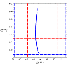
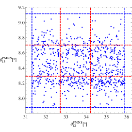
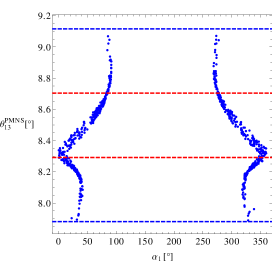
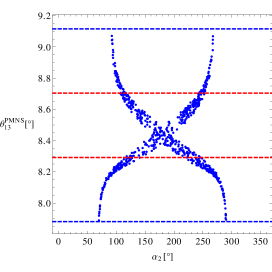
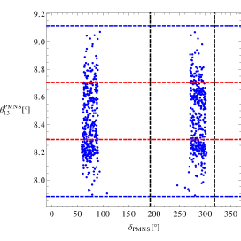
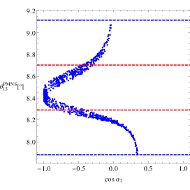
Figure 1: Results of our parameter scan for the normal hierarchy (blue points). The allowed experimental 3$\sigma$ (1$\sigma$) regions are limited by blue (red) dashed lines. The black dashed lines represent the 1$\sigma$ range for the not directly measured CP phase $\delta_{\text{PMNS}}$ from the global fit [8].

Our numerical scan results for the leptonic mixing parameters are displayed in Fig. 1, where the allowed 3$\sigma$ (1$\sigma$) regions are limited by blue (red) dashed lines. The black dashed lines represent the 1$\sigma$ range for the not directly measured CP phase $\delta_{\text{PMNS}}$ from the global fit [8]. The blue points are the result from our parameter scan to which we have applied the experimental data as constraints.

Note that $\theta_{23}^{\text{PMNS}}$ is not within the 1$\sigma$ region. And hence, if it is confirmed that the atmospheric mixing is not close to maximal this concrete model would be ruled out. Nevertheless, it is rather straightforward to introduce a $\theta_{23}^{e}$ mixing which would allow to fit $\theta_{23}^{\text{PMNS}}$ but would make the model much less predictive.

For the Majorana phases $\alpha_{1}$ and $\alpha_{2}$ we find values between $0^{\circ}$–$90^{\circ}$ or $270^{\circ}$–$360^{\circ}$ for $\alpha_{1}$ and $70^{\circ}$–$290^{\circ}$ for $\alpha_{2}$. We find the Dirac phase $\delta_{\text{PMNS}}$ to be in the region from $57^{\circ}$–$108^{\circ}$ or $244^{\circ}$–$303^{\circ}$. The Jarlskog invariant which determines the CP violation in neutrino oscillations is given by [48]

$$J_{\text{CP}}=\text{Im}(U_{\mu 3}U_{e3}^{*}U_{e2}U_{\mu 2}^{*})=\frac{1}{8}\cos(\theta_{13}^{\text{PMNS}})\sin(2\theta_{12}^{\text{PMNS}})\sin(2\theta_{13}^{\text{PMNS}})\sin(2\theta_{23}^{\text{PMNS}})\sin{\delta_{\text{PMNS}}}.$$ (3.43)

We obtain $J_{\text{CP}}\approx\pm(0.027-0.035)$.

We would like to mention here the work done in [49] where among other things a similar setup was studied and constraints for the phases were found. Nevertheless, the authors neglected RGE running effects which they can do by assuming a small $\tan\beta$ or no supersymmetry at all and furthermore they have no mass sum rule and therefore neutrino masses can be light in their setup. Nevertheless, in the normal hierarchical setup where RGE effects do not have a large impact we find similar results.

As we mentioned before the mass sum rule only implies a lower bound for the mass scale for the normal hierarchy. But here we find as well an upper bound due to the constraint that $\theta_{13}^{\text{PMNS}}$ should stay within the experimental 3$\sigma$ region. This can be clearly seen in the last plot in Fig. 1 where we have plotted $\cos\left(\alpha_{2}\right)$ against $\theta_{13}^{\text{PMNS}}$. The mass sum rule implies $\cos\left(\alpha_{2}\right)$ to be in the range from $-1$ to about $0.48$, where larger values imply larger masses and larger RGE corrections to $\theta_{13}^{\text{PMNS}}$.

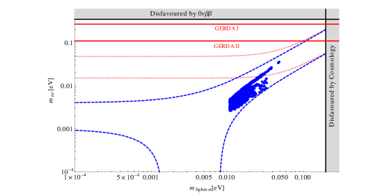
Figure 2: Prediction for the effective neutrino mass $m_{ee}$ accessible in neutrinoless double beta decay experiments as a function of the lightest neutrino mass $m_{1}$. The blue dashed region represents the allowed region for normal ordering whereas the pink dotted region indicates the inverted ordering region which is not allowed in our setup. The grey region on the right side shows the bounds on the lightest mass from cosmology [52] and the grey region in the upper part displays the upper bound on the effective mass from the EXO experiment [51]. The red lines represent the sensitivity of GERDA phase I respectively GERDA phase II [50].

The effective neutrino mass accessible in neutrinoless double beta decay experiments like GERDA [50] or EXO [51] is given by

$$\left|m_{ee}\right|=\left|m_{1}U_{e1}^{2}+m_{2}U_{e2}^{2}+m_{3}U_{e3}^{2}\right|=\left|m_{1}c_{12}^{2}c_{13}^{2}\text{e}^{-\text{i}\alpha_{1}}+m_{2}s_{12}^{2}c_{13}^{2}\text{e}^{-\text{i}\alpha_{2}}+m_{3}s_{13}^{2}\text{e}^{-\text{i}2\delta_{\text{PMNS}}}\right|.$$ (3.44)

A graphically representation of our prediction for $m_{ee}$ as a function of $m_{1}$ is shown in Fig. 2. We find values for $m_{ee}$ in the range from 0.02 eV to 0.04 eV corresponding to the lightest neutrino mass $m_{1}$ in the region from 0.01 eV to 0.05 eV. This results are beyond the sensitivity of the GERDA experiment but might be tested by a future experiment.

With the value for the lightest neutrino mass $m_{1}$ between about 0.01 eV and 0.05 eV and the experimental mass squared differences from Tab. 1 we obtain for the sum of the neutrino masses $\sum m_{\nu}=(0.074$–0.171) eV. This prediction is compatible with the cosmological bound for the sum of the neutrino masses [52]

$$\sum m_{\nu}<0.23\text{ eV.}$$ (3.45)

The quantity which will be measured in the experiment KATRIN [53] is the kinematic neutrino mass $m_{\beta}$ which is given as

$$m_{\beta}^{2}=m_{1}^{2}c_{12}^{2}c_{13}^{2}+m_{2}^{2}s_{12}^{2}c_{13}^{2}+m_{3}^{2}s_{13}^{2}.$$ (3.46)

Applying the range for $m_{1}$ as well as the measured mass squared differences we arrive at $m_{\beta}\approx(0.014$–$0.052)$ eV. Regarding the sensitivity of the experiment which is $m_{\beta}>0.2$ eV our model prediction is beyond the reach of KATRIN.

4 Summary and Conclusions

In this paper we have presented the first SU(5)$\,\times\,$ A₅ SUSY Flavour Model to our knowledge. It features to leading order the appealing prediction $\theta_{12}^{\text{PMNS}}=\tan^{-1}\left(\frac{1}{\phi_{g}}\right)\approx 31.7^{\circ}$ where $\phi_{g}$ is the golden ratio $\phi_{g}=(1+\sqrt{5})/2$. The reactor mixing angle is predicted to be vanishing at leading order and the atmospheric mixing angle to be maximal. Furthermore, the neutrino masses exhibit a sum rule, which turns out to be very important for the phenomenology.

The prediction of a vanishing reactor mixing angle is excluded by several standard deviations and hence the leading order predictions have to be corrected to make the model seem realistic. In grand unified theories nevertheless, it is natural to expect that the charged lepton Yukawa matrix is not diagonal because it is related to the down-type quark sector which is well motivated to be non-diagonal in flavour space. This is furthermore suggested by the approximate relation $\theta_{13}^{\text{PMNS}}\approx\theta_{C}/\sqrt{2}$, where $\theta_{C}$ is the Cabibbo angle. But in our setup we do not only have relations between quark and lepton mixing angles, but also between down-type quark and charged lepton Yukawa couplings which are non-standard, $y_{\tau}/y_{b}\approx-1.5$ and $y_{\mu}/y_{s}\approx 6$, and for the double ratio $(y_{\mu}/y_{s})(y_{d}/y_{e})=12$ which are all in perfect agreement with experimental data. The Yukawa coupling ratios for the third and second generation put furthermore two non-trivial constraints on the SUSY spectrum which might be tested at the LHC or one of its successors.

To achieve the desired Yukawa coupling ratios and a non-diagonal charged lepton Yukawa matrix we have presented a complete symmetry breaking sector for SU(5) and A₅. The SU(5) breaking sector is peculiar because it is in principle compatible with the double missing partner mechanism as discussed in [29], a mechanism to decouple the coloured triplets and hence suppress proton decay sufficiently. In the A₅ symmetry breaking we have introduced a few non-trivial representations which break A₅ in the desired groups such that we end up with golden ratio mixing type A to leading order in the neutrino sector including also a sum rule for the neutrino masses. We have also studied a messenger sector for the model which is important for choosing between different Yukawa coupling relations in the effective higher-dimensional operators and forbidding other unwanted effective operators which might be allowed by the symmetries alone.

Apart from corrections from the charged lepton sector, RGE corrections can also play a major role. In fact, RGE corrections rule out the inverted neutrino mass hierarchy. The neutrino mass sum rule allows both mass hierarchies but in both cases only a certain mass range. For inverted hierarchy the neutrino masses turn out to be rather heavy and since $\tan\beta$ is as well rather large the RGE corrections to $\theta_{12}^{\text{PMNS}}$ are so large that although at the high scale we are at most a few degrees away from the observed value at low energies we are far outside the allowed 3$\sigma$ region for $\theta_{12}^{\text{PMNS}}$. Hence, only the normal hierarchy is possible in our model setup and we find all three mixing angles to be in the 3$\sigma$ regions and $J_{\text{CP}}\approx\pm 0.03$ with the lightest neutrino mass $m_{1}\approx 0.01$–$0.05$ eV. Due to the mass and angle sum rules we also find constraints on the phases, most phenomenologically relevant for the near future, $\delta_{\text{PMNS}}$ to be in the region from $57^{\circ}$–$108^{\circ}$ or $244^{\circ}$–$303^{\circ}$.

Hence, our model can be tested from neutrino and collider experiments in several different ways in the near future.

Note Added

During the finalisation of this work an update of the nu-fit global fitting collaboration appeared [54]. Nevertheless, the results which we used in our analysis changed only very little compared to their updated fit and hence our conclusions remain unchanged.

Appendix A The messenger sector

In this section we discuss the renormalisable superpotential of the model. As mentioned before the heavy messenger fields are integrated out to obtain the higher dimensional operators of the effective superpotential. The complete messenger field content can be found in Tabs. 6 and 7.

	$\mathrm{SU(5)}$	$\mathrm{A_{5}}$	$\mathbb{Z}_{4}^{R}$	$\mathbb{Z}_{2}$	$\mathbb{Z}_{2}$	$\mathbb{Z}_{3}$	$\mathbb{Z}_{3}$	$\mathbb{Z}_{3}$	$\mathbb{Z}_{3}$	$\mathbb{Z}_{3}$	$\mathbb{Z}_{3}$	$\mathbb{Z}_{4}$
$\Sigma_{1}$	$\mathbf{5}$	$\mathbf{3}$	$1$	$0$	$0$	$2$	$1$	$2$	$1$	$0$	$1$	$0$
$\bar{\Sigma}_{1}$	$\mathbf{\bar{5}}$	$\mathbf{3}$	$1$	$0$	$0$	$1$	$2$	$1$	$2$	$0$	$2$	$0$
$\Sigma_{2}$	$\mathbf{5}$	$\mathbf{1}$	$1$	$0$	$0$	$2$	$1$	$1$	$2$	$0$	$1$	$3$
$\bar{\Sigma}_{2}$	$\mathbf{\bar{5}}$	$\mathbf{1}$	$1$	$0$	$0$	$1$	$2$	$2$	$1$	$0$	$2$	$1$
$\Xi_{1}$	$\mathbf{45}$	$\mathbf{3}$	$1$	$0$	$0$	$2$	$1$	$2$	$1$	$0$	$1$	$0$
$\bar{\Xi}_{1}$	$\mathbf{\bar{45}}$	$\mathbf{3}$	$1$	$0$	$0$	$1$	$2$	$1$	$2$	$0$	$2$	$0$
$\Xi_{2}$	$\mathbf{45}$	$\mathbf{3}$	$1$	$0$	$1$	$2$	$1$	$1$	$1$	$2$	$0$	$1$
$\bar{\Xi}_{2}$	$\mathbf{\bar{45}}$	$\mathbf{3}$	$1$	$0$	$1$	$1$	$2$	$2$	$2$	$1$	$0$	$3$
$\Xi_{3}$	$\mathbf{45}$	$\mathbf{1}$	$1$	$1$	$0$	$2$	$2$	$1$	$2$	$0$	$0$	$0$
$\bar{\Xi}_{3}$	$\mathbf{\bar{45}}$	$\mathbf{1}$	$1$	$1$	$0$	$1$	$1$	$2$	$1$	$0$	$0$	$0$
$\Xi_{4}$	$\mathbf{45}$	$\mathbf{1}$	$2$	$0$	$0$	$0$	$0$	$1$	$0$	$0$	$0$	$0$
$\bar{\Xi}_{4}$	$\mathbf{\bar{45}}$	$\mathbf{1}$	$0$	$0$	$0$	$0$	$0$	$2$	$0$	$0$	$0$	$0$
$\Gamma_{1}$	$\mathbf{1}$	$\mathbf{3}$	$0$	$0$	$0$	$0$	$1$	$1$	$1$	$0$	$0$	$0$
$\bar{\Gamma}_{1}$	$\mathbf{1}$	$\mathbf{3}$	$2$	$0$	$0$	$0$	$2$	$2$	$2$	$0$	$0$	$0$
$\Gamma_{2}$	$\mathbf{1}$	$\mathbf{3}$	$0$	$0$	$0$	$0$	$1$	$2$	$0$	$0$	$0$	$1$
$\bar{\Gamma}_{2}$	$\mathbf{1}$	$\mathbf{3}$	$2$	$0$	$0$	$0$	$2$	$1$	$0$	$0$	$0$	$3$
$\Gamma_{3}$	$\mathbf{1}$	$\mathbf{1}$	$0$	$0$	$0$	$2$	$2$	$2$	$0$	$0$	$0$	$0$
$\bar{\Gamma}_{3}$	$\mathbf{1}$	$\mathbf{1}$	$2$	$0$	$0$	$0$	$1$	$1$	$1$	$0$	$0$	$0$
$\Omega_{1}$	$\mathbf{10}$	$\mathbf{1}$	$1$	$0$	$0$	$0$	$1$	$0$	$0$	$0$	$0$	$3$
$\bar{\Omega}_{1}$	$\mathbf{\bar{10}}$	$\mathbf{1}$	$1$	$0$	$0$	$0$	$2$	$0$	$0$	$0$	$0$	$1$
$\Omega_{2}$	$\mathbf{10}$	$\mathbf{1}$	$1$	$1$	$0$	$2$	$0$	$0$	$0$	$0$	$0$	$0$
$\bar{\Omega}_{2}$	$\mathbf{\bar{10}}$	$\mathbf{1}$	$1$	$1$	$0$	$1$	$0$	$0$	$0$	$0$	$0$	$0$
$\Omega_{3}$	$\mathbf{10}$	$\mathbf{1}$	$1$	$1$	$0$	$2$	$2$	$0$	$0$	$0$	$0$	$3$
$\bar{\Omega}_{3}$	$\mathbf{\bar{10}}$	$\mathbf{1}$	$1$	$1$	$0$	$1$	$1$	$0$	$0$	$0$	$0$	$1$
$\Omega_{4}$	$\mathbf{10}$	$\mathbf{1}$	$1$	$1$	$0$	$1$	$1$	$2$	$2$	$0$	$0$	$2$
$\bar{\Omega}_{4}$	$\mathbf{\bar{10}}$	$\mathbf{1}$	$1$	$1$	$0$	$2$	$2$	$1$	$1$	$0$	$0$	$2$
$\Omega_{5}$	$\mathbf{10}$	$\mathbf{3}$	$1$	$0$	$0$	$1$	$2$	$0$	$1$	$0$	$2$	$0$
$\bar{\Omega}_{5}$	$\mathbf{\bar{10}}$	$\mathbf{3}$	$1$	$0$	$0$	$2$	$1$	$0$	$2$	$0$	$1$	$0$
$\Omega_{6}$	$\mathbf{10}$	$\mathbf{1}$	$1$	$0$	$0$	$1$	$1$	$1$	$1$	$0$	$2$	$3$
$\bar{\Omega}_{6}$	$\mathbf{\bar{10}}$	$\mathbf{1}$	$1$	$0$	$0$	$2$	$2$	$2$	$2$	$0$	$1$	$1$
$\Omega_{7}$	$\mathbf{10}$	$\mathbf{3}$	$1$	$0$	$0$	$1$	$1$	$2$	$0$	$0$	$2$	$0$
$\bar{\Omega}_{7}$	$\mathbf{\bar{10}}$	$\mathbf{3}$	$1$	$0$	$0$	$2$	$2$	$1$	$0$	$0$	$1$	$0$

Table 6: The $\mathbb{Z}_{n}$ charges, $\mathrm{SU(5)}$ and $\mathrm{A_{5}}$ representations of the messenger fields for the Yukawa couplings.

	$\mathrm{SU(5)}$	$\mathrm{A_{5}}$	$\mathbb{Z}_{4R}$	$\mathbb{Z}_{2}$	$\mathbb{Z}_{2}$	$\mathbb{Z}_{3}$	$\mathbb{Z}_{3}$	$\mathbb{Z}_{3}$	$\mathbb{Z}_{3}$	$\mathbb{Z}_{3}$	$\mathbb{Z}_{3}$	$\mathbb{Z}_{4}$
$\Upsilon_{\epsilon 2}$	$\mathbf{1}$	$\mathbf{1}$	$2$	$0$	$0$	$0$	$2$	$0$	$0$	$0$	$0$	$2$
$\bar{\Upsilon}_{\epsilon 2}$	$\mathbf{1}$	$\mathbf{1}$	$0$	$0$	$0$	$0$	$1$	$0$	$0$	$0$	$0$	$2$
$\Upsilon_{\epsilon 3}$	$\mathbf{1}$	$\mathbf{1}$	$2$	$0$	$0$	$1$	$2$	$0$	$0$	$0$	$0$	$0$
$\bar{\Upsilon}_{\epsilon 3}$	$\mathbf{1}$	$\mathbf{1}$	$0$	$0$	$0$	$2$	$1$	$0$	$0$	$0$	$0$	$0$
$\Upsilon_{\epsilon 4}$	$\mathbf{1}$	$\mathbf{1}$	$2$	$0$	$0$	$2$	$2$	$2$	$2$	$0$	$0$	$2$
$\bar{\Upsilon}_{\epsilon 4}$	$\mathbf{1}$	$\mathbf{1}$	$0$	$0$	$0$	$1$	$1$	$1$	$1$	$0$	$0$	$2$
$\Upsilon_{\epsilon 5}$	$\mathbf{1}$	$\mathbf{1}$	$2$	$0$	$0$	$1$	$0$	$2$	$2$	$0$	$0$	$2$
$\bar{\Upsilon}_{\epsilon 5}$	$\mathbf{1}$	$\mathbf{1}$	$0$	$0$	$0$	$2$	$0$	$1$	$1$	$0$	$0$	$2$
$\Upsilon_{\theta 1}$	$\mathbf{1}$	$\mathbf{1}$	$2$	$0$	$0$	$0$	$2$	$2$	$1$	$1$	$0$	$0$
$\bar{\Upsilon}_{\theta 1}$	$\mathbf{1}$	$\mathbf{1}$	$0$	$0$	$0$	$0$	$1$	$1$	$2$	$2$	$0$	$0$
$\Upsilon_{\theta 2}$	$\mathbf{1}$	$\mathbf{1}$	$2$	$0$	$0$	$0$	$2$	$1$	$2$	$1$	$0$	$2$
$\bar{\Upsilon}_{\theta 2}$	$\mathbf{1}$	$\mathbf{1}$	$0$	$0$	$0$	$0$	$1$	$2$	$1$	$2$	$0$	$2$
$\Upsilon_{\theta 3}$	$\mathbf{1}$	$\mathbf{1}$	$2$	$0$	$0$	$0$	$0$	$1$	$0$	$1$	$1$	$2$
$\bar{\Upsilon}_{\theta 3}$	$\mathbf{1}$	$\mathbf{1}$	$0$	$0$	$0$	$0$	$0$	$2$	$0$	$2$	$2$	$2$
$\Lambda_{\epsilon 2}$	$\mathbf{1}$	$\mathbf{1}$	$2$	$0$	$0$	$0$	$1$	$0$	$0$	$0$	$0$	$0$
$\bar{\Lambda}_{\epsilon 2}$	$\mathbf{1}$	$\mathbf{1}$	$0$	$0$	$0$	$0$	$2$	$0$	$0$	$0$	$0$	$0$
$\Lambda_{\epsilon 4}$	$\mathbf{1}$	$\mathbf{1}$	$2$	$0$	$0$	$1$	$1$	$1$	$1$	$0$	$0$	$0$
$\bar{\Lambda}_{\epsilon 4}$	$\mathbf{1}$	$\mathbf{1}$	$0$	$0$	$0$	$2$	$2$	$2$	$2$	$0$	$0$	$0$
$\Lambda_{\epsilon 5}$	$\mathbf{1}$	$\mathbf{1}$	$2$	$0$	$0$	$2$	$0$	$1$	$1$	$0$	$0$	$0$
$\bar{\Lambda}_{\epsilon 5}$	$\mathbf{1}$	$\mathbf{1}$	$0$	$0$	$0$	$1$	$0$	$2$	$2$	$0$	$0$	$0$
$\Lambda_{\theta 2}$	$\mathbf{1}$	$\mathbf{1}$	$2$	$0$	$0$	$0$	$1$	$2$	$1$	$2$	$0$	$0$
$\bar{\Lambda}_{\theta 2}$	$\mathbf{1}$	$\mathbf{1}$	$0$	$0$	$0$	$0$	$2$	$1$	$2$	$1$	$0$	$0$
$\Lambda_{\theta 3}$	$\mathbf{1}$	$\mathbf{1}$	$2$	$0$	$0$	$0$	$0$	$2$	$0$	$2$	$2$	$0$
$\bar{\Lambda}_{\theta 3}$	$\mathbf{1}$	$\mathbf{1}$	$0$	$0$	$0$	$0$	$0$	$1$	$0$	$1$	$1$	$0$
$\Delta_{\epsilon 2}$	$\mathbf{1}$	$\mathbf{1}$	$2$	$0$	$0$	$0$	$2$	$0$	$0$	$0$	$0$	$0$
$\bar{\Delta}_{\epsilon 2}$	$\mathbf{1}$	$\mathbf{1}$	$0$	$0$	$0$	$0$	$1$	$0$	$0$	$0$	$0$	$0$
$\Delta_{\epsilon 3}$	$\mathbf{1}$	$\mathbf{1}$	$2$	$0$	$0$	$2$	$1$	$0$	$0$	$0$	$0$	$0$
$\bar{\Delta}_{\epsilon 3}$	$\mathbf{1}$	$\mathbf{1}$	$0$	$0$	$0$	$1$	$2$	$0$	$0$	$0$	$0$	$0$
$\Delta_{\epsilon 4}$	$\mathbf{1}$	$\mathbf{1}$	$2$	$0$	$0$	$2$	$2$	$2$	$2$	$0$	$0$	$0$
$\bar{\Delta}_{\epsilon 4}$	$\mathbf{1}$	$\mathbf{1}$	$0$	$0$	$0$	$1$	$1$	$1$	$1$	$0$	$0$	$0$
$\Delta_{\epsilon 5}$	$\mathbf{1}$	$\mathbf{1}$	$2$	$0$	$0$	$1$	$0$	$2$	$2$	$0$	$0$	$0$
$\bar{\Delta}_{\epsilon 5}$	$\mathbf{1}$	$\mathbf{1}$	$0$	$0$	$0$	$2$	$0$	$1$	$1$	$0$	$0$	$0$
$\Delta_{\theta 1}$	$\mathbf{1}$	$\mathbf{1}$	$2$	$0$	$0$	$0$	$1$	$1$	$2$	$2$	$0$	$0$
$\bar{\Delta}_{\theta 1}$	$\mathbf{1}$	$\mathbf{1}$	$0$	$0$	$0$	$0$	$2$	$2$	$1$	$1$	$0$	$0$
$\Delta_{\theta 2}$	$\mathbf{1}$	$\mathbf{1}$	$2$	$0$	$0$	$0$	$2$	$1$	$2$	$1$	$0$	$0$
$\bar{\Delta}_{\theta 2}$	$\mathbf{1}$	$\mathbf{1}$	$0$	$0$	$0$	$0$	$1$	$2$	$1$	$2$	$0$	$0$
$\Delta_{\theta 3}$	$\mathbf{1}$	$\mathbf{1}$	$2$	$0$	$0$	$0$	$0$	$1$	$0$	$1$	$1$	$0$
$\bar{\Delta}_{\theta 3}$	$\mathbf{1}$	$\mathbf{1}$	$0$	$0$	$0$	$0$	$0$	$2$	$0$	$2$	$2$	$0$

Table 7: The $\mathbb{Z}_{n}$ charges, $\mathrm{SU(5)}$ and $\mathrm{A_{5}}$ representations of the messenger fields for the flavon sector.

We will first discuss the renormalisable superpotentials for the up- and down-type quark sectors including additional operators not seen in our supergraphs but allowed by symmetry. We will then do the same for the flavon sector. At last we will discuss higher dimensional operators.

We begin with the mass terms for the messenger fields

$$\begin{split}\mathcal{W}_{\Lambda}^{\text{ren}}&=M_{\Sigma_{i}}\Sigma_{i}\bar{\Sigma}_{i}+M_{\Omega_{i}}\Omega_{i}\bar{\Omega_{i}}+M_{\Xi_{i}}\Xi_{i}\bar{\Xi}_{i}+M_{\Gamma_{i}}\Gamma_{i}\bar{\Gamma}_{i}+M_{\Upsilon_{f6}}\Upsilon_{f6}\bar{\Upsilon}_{f6}\\ &+M_{\Delta_{f6}}\Delta_{f6}\bar{\Delta}_{f6}+M_{\Upsilon_{f12}}\Upsilon_{f12}\bar{\Upsilon}_{f12}+M_{\Delta_{f12}}\Delta_{f12}\bar{\Delta}_{f12}+M_{\Lambda_{f12}}\Lambda_{f12}\bar{\Lambda}_{f12}\;,\end{split}$$ (A.1)

where a summation over $i$ is implied. The indices $f6$ and $f12$ denote the singlet flavons which occur as 6th and 12th power respectively in their aligning superpotentials. It is $f6\in\{\theta_{1},\epsilon_{3}\}$ and $f12\in\{\theta_{2},\theta_{3},\epsilon_{2},\epsilon_{4},\epsilon_{5}\}$ where a summation over these flavons is implied. Each messenger field has a mass higher than the GUT scale. The individual messenger masses are related to the messenger mass scale $\Lambda$ by order one coefficients which are often not explicitly stated to simplify the notation.

The renormalisable superpotential for the up-quark sector is

$$\begin{split}\mathcal{W}_{u}^{\text{ren}}&=T_{3}T_{3}H_{5}+T_{3}\epsilon_{1}\bar{\Omega}_{1}+\Omega_{1}T_{2}H_{5}+\epsilon_{1}^{2}\bar{\Gamma}_{3}+\Gamma_{3}T_{2}\bar{\Omega}_{1}+\epsilon_{1}T_{1}\bar{\Omega}_{2}\\ &+\Omega_{2}\epsilon_{2}\bar{\Omega}_{3}+\Omega_{3}\bar{\Omega}_{1}\epsilon_{3}+\Omega_{3}\bar{\Omega}_{4}\epsilon_{4}+\Omega_{4}T_{1}H_{5}+\bar{\Omega}_{4}\Omega_{1}\epsilon_{5}\;,\end{split}$$ (A.2)

where the coupling constants have been ommitted to increase clarity. The supergraphs for this sector can be found in Fig. 3. In order to get the effective operators in section 2, the messenger fields have to be integrated out.

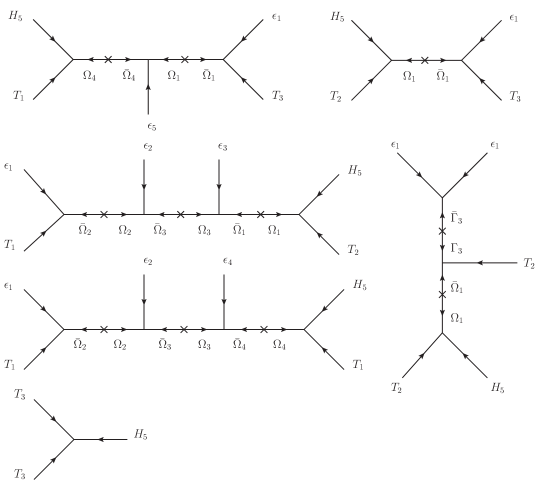
Figure 3: The supergraphs before integrating out the heavy messenger field for the up-type quark sector.

The renormalisable superpotential for the charged lepton and down-type quark sector is

$$\begin{split}\mathcal{W}_{d,l}^{\text{ren}}&=H_{24}F\Sigma_{1}+\bar{\Sigma}_{1}\phi_{2}\Sigma_{2}+\bar{\Sigma}_{2}T_{3}\bar{H}_{5}+FH_{24}\Xi_{1}+\bar{\Xi}_{1}\theta_{3}\Xi_{2}\\ &+\bar{\Xi}_{2}\phi_{3}\Xi_{3}+\bar{\Xi}_{3}\bar{\Xi}_{4}T_{1}+\Xi_{4}\bar{H}_{5}H_{24}\\ &+F\bar{H}_{5}\Omega_{5}+\bar{\Omega}_{5}\Omega_{6}\Gamma_{2}+\bar{\Omega}_{6}H_{24}T_{2}+\bar{\Gamma}_{2}\phi_{3}\theta_{1}\\ &+\bar{\Omega}_{5}\Omega_{7}\Gamma_{1}+\bar{\Gamma}_{1}\theta_{2}\phi_{3}+\bar{\Omega}_{7}\Omega_{6}\phi_{2}+\bar{\Omega}_{5}\Omega_{7}\epsilon_{1}\;,\end{split}$$ (A.3)

where again coupling constants have been omitted. The charges under the shaping symmetries are listed in Tab. 6 for the messenger fields and Tab. 3 for the matter and Higgs fields of the model. The supergraphs for this sector can be found in Fig. 4. There are a few additional couplings which are not forbidden by shaping symmetries. These are

$$\mathcal{W}_{\text{additional}} =\bar{\Gamma}_{3}^{3}+\bar{\Gamma}_{3}\Gamma_{1}^{2}+\Gamma_{3}\Omega_{5}\bar{\Omega}_{7}+\Gamma_{1}\bar{\Gamma}_{2}\phi_{2}+\bar{\Gamma}_{2}\epsilon_{1}\phi_{2}\;.$$ (A.4)

It is important to note that the vertices above which contain $\Gamma_{3}$ or $\epsilon_{1}$ and any messenger field of the down-sector are the only allowed couplings that mix messenger fields of the up- and down-sector. We will discuss the implications of these terms on potential higher dimensional operators later.

The operator $\bar{\Gamma}_{2}\phi_{2}\epsilon_{1}$ generates a second leading order diagram for the 3-2 element of $Y_{d}$ (and the 2-3 element of $Y_{e}$ respectively). Since it generates the same effective operator as the supergraph shown in Fig. 4 with the same CG coefficient in the charged lepton sector, we have omitted the diagram. The same reasoning applies to the term $\Gamma_{1}\bar{\Gamma}_{2}\phi_{2}$ which generates a second leading order diagram for the 1-2 element of $Y_{d}$ (and the 2-1 element of $Y_{e}$ respectively).

There are more couplings between the messenger fields of the singlet flavons. These will be further discussed below, since there are no couplings mixing the singlet messenger fields with messenger fields from any other sector.

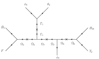
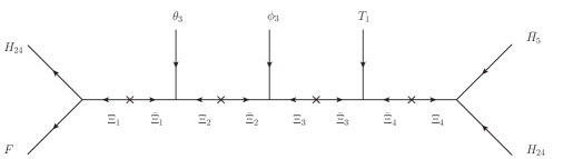
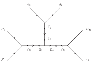
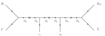
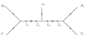
Figure 4: The supergraphs for the down-type quark and charged lepton sector.

In the flavon sector only the singlet alignment requires the introduction of new messenger fields, since the superpotential for the flavon fields in the three-, four- and five-dimensional representations of $\mathrm{A}_{5}$ is already renormalisable. The messenger fields for the flavon sector and their charges under the various symmetries of the model can be found in Tab. 7. For $\epsilon_{1}$ the renormalisable superpotential reads

$$\mathcal{W}_{s3}^{\text{ren}} =\epsilon_{1}^{2}\bar{\Gamma}_{3}+P\epsilon_{1}\Gamma_{3}\;.$$ (A.5)

The renormalisable superpotentials of $\epsilon_{3}$ and $\theta_{1}$ are of the form

$$\mathcal{W}_{s6}^{\text{ren}} =f_{i}^{2}\Upsilon_{fi}+\bar{\Upsilon}_{fi}^{2}\Delta_{fi}+P\bar{\Delta}_{fi}\bar{\Upsilon}_{fi}\;,$$ (A.6)

where $f_{i}$ denotes one of the above mentioned flavons. After integrating out the heavy messenger fields we get an effective operator which contains the respective flavon to the power of six. The remaining singlets have superpotentials of the form

$$\mathcal{W}_{s12}^{\text{ren}} =f_{i}^{2}\Upsilon_{fi}+\bar{\Upsilon}_{fi}^{2}\Lambda_{fi}+\bar{\Lambda}_{fi}^{2}\Delta_{fi}+P\bar{\Delta}_{fi}\bar{\Lambda}_{fi}\;,$$ (A.7)

where $f_{i}$ again denotes one of the mentioned flavons. This superpotential results in an effective operator containing the singlet flavon to the power of 12. The corresponding supergraphs can be found in Fig. 5.

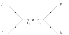
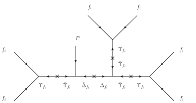
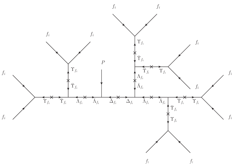
Figure 5: The supergraphs for the sector of the singlet flavons.

As already discussed in the matter sector there are additional couplings among the messenger fields of the flavon sector not forbidden by symmetry. However, note that these messenger fields do not couple to any other sector with the exception of one term which will be discussed in detail later. These terms will not be displayed here, since they do not lead to new leading order effective operators. We have checked this already on the effective level without resorting to messenger selection rules.

The only non-trivial operator left to discuss is $D_{\phi}^{(2)}\Upsilon_{\theta_{2}}\Delta_{\theta_{1}}$ which generates an effective operator $D_{\phi}^{(2)}P^{2}\theta_{1}^{2}\theta_{2}^{10}$ which nevertheless, due to the vanishing of $\langle P\rangle$, does not have any effect whatsoever.

We turn now to the additional effective operators for the Yukawa matrices. It is useful to recall their structure here to leading order. In the down-type quark and charged lepton sector we have

$$Y_{d}^{\text{LO}} =\begin{pmatrix}0&\Lambda^{-4}&0\\ \Lambda^{-4}&\Lambda^{-3}&0\\ 0&\Lambda^{-3}&\Lambda^{-2}\\ \end{pmatrix}\;,$$ (A.8)

and in the up-type quark sector

$$Y_{u}^{\text{LO}} =\begin{pmatrix}\Lambda^{-3}&\Lambda^{-3}&\Lambda^{-2}\\ \Lambda^{-3}&\Lambda^{-2}&\Lambda^{-1}\\ \Lambda^{-2}&\Lambda^{-1}&1\\ \end{pmatrix}\;.$$ (A.9)

For both sectors we have checked for possible additional effective operators using only the symmetries of the model, i.e. without considering messenger fields. In the up-type quark sector the largest corrections come from operators with a mass dimension at least two higher than the leading order operator. We therefore have $Y_{u}=Y_{u}^{\text{LO}}+Y_{u}^{\text{HO}}$, where

$$Y_{u}^{\text{HO}} \lesssim\begin{pmatrix}\Lambda^{-6}&\Lambda^{-6}&\Lambda^{-5}\\ \Lambda^{-6}&\Lambda^{-5}&\Lambda^{-4}\\ \Lambda^{-5}&\Lambda^{-4}&\Lambda^{-3}\\ \end{pmatrix}\;.$$ (A.10)

Hence, we can neglect them.

In the down-type quark sector we have as well calculated higher order effective operators based on symmetry arguments only, where operators containing $\phi_{2}^{2}$ or $\phi_{3}^{2}$ where ignored, because $\langle\phi_{2}\rangle^{2}=\langle\phi_{3}\rangle^{2}=0$. We find five additional effective operators

$$\begin{split}\mathcal{W}^{\text{HO}}&=\frac{1}{\Lambda^{4}}H_{24}\bar{H}_{5}FT_{1}\phi_{2}\epsilon_{3}\epsilon_{2}+\frac{1}{\Lambda^{4}}H_{24}\bar{H}_{5}FT_{1}\phi_{2}\epsilon_{5}\epsilon_{1}+\frac{1}{\Lambda^{4}}H_{24}\bar{H}_{5}FT_{1}\phi_{3}\epsilon_{5}\theta_{1}\\ &+\frac{1}{\Lambda^{5}}H_{24}\bar{H}_{5}FT_{1}\phi_{2}\phi_{3}\theta_{2}\epsilon_{5}+\frac{1}{\Lambda^{5}}H_{24}\bar{H}_{5}FT_{3}\phi_{3}\theta_{1}\epsilon_{1}\epsilon_{1}\;.\end{split}$$ (A.11)

Upon close inspection of the terms in eq. (A.11) it becomes clear, that those terms are forbidden due to messenger arguments. As stated above there are no couplings other than to $\Gamma_{3}$ and $\epsilon_{1}$ that mix up-type quark and down-type quark messenger fields. Since $\epsilon_{5}$ and $\epsilon_{3}$ do not immediately couple to $\Gamma_{3}$ it is impossible to generate the terms containing only those flavons, since further external legs from the up-sector would arise. The last term in eq. (A.11) cannot be realised since $T_{3}$ couples only to $\bar{\Sigma}_{2}$, a messenger field in the $\mathbf{\bar{5}}$ representation of SU(5). There are no couplings mixing this messenger field with any of the fields in other representations of SU(5), making the effective operator containing $T_{3}$ and $\epsilon_{1}$ impossible.

In conclusion we found for the down-type Yukawa matrix $Y_{d}=Y_{d}^{\text{LO}}+Y_{d}^{\text{HO}}$

$$Y_{d}^{\text{HO}} \lesssim\begin{pmatrix}\Lambda^{-6}&\Lambda^{-6}&\Lambda^{-6}\\ \Lambda^{-6}&\Lambda^{-6}&\Lambda^{-6}\\ \Lambda^{-6}&\Lambda^{-6}&\Lambda^{-5}\\ \end{pmatrix}\;,$$ (A.12)

which can again be safely neglected.

Appendix B A₅ Clebsch-Gordan Coefficients

For convenience we give here the Clebsch-Gordan coefficients of the group A₅, taken from [13]. We use the notation $a_{i}$ ($b_{i}$) for elements of the first (second) representation. The subscript $a$ ($s$) denotes antisymmetric (symmetric) representations.

$\mathbf{3}\otimes\mathbf{3}=\mathbf{1_{s}}\oplus\mathbf{3_{a}}\oplus\mathbf{5_{s}}$	$\mathbf{3^{\prime}}\otimes\mathbf{3^{\prime}}=\mathbf{1_{s}}\oplus\mathbf{3_{a}^{\prime}}\oplus\mathbf{5_{s}}$
$\mathbf{1_{s}}\sim a_{1}b_{1}+a_{2}b_{3}+a_{3}b_{2}$	$\mathbf{1_{s}}\sim a_{1}b_{1}+a_{2}b_{3}+a_{3}b_{2}$
$\mathbf{3_{a}}\sim\begin{pmatrix}a_{2}b_{3}-a_{3}b_{2}\\ a_{1}b_{2}-a_{2}b_{1}\\ a_{3}b_{1}-a_{1}b_{3}\\ \end{pmatrix}$	$\mathbf{3_{a}}^{\prime}\sim\begin{pmatrix}a_{2}b_{3}-a_{3}b_{2}\\ a_{1}b_{2}-a_{2}b_{1}\\ a_{3}b_{1}-a_{1}b_{3}\\ \end{pmatrix}$
$\mathbf{5_{s}}\sim\begin{pmatrix}2a_{1}b_{1}-a_{2}b_{3}-a_{3}b_{2}\\ -\sqrt{3}a_{1}b_{2}-\sqrt{3}a_{2}b_{1}\\ \sqrt{6}a_{2}b_{2}\\ \sqrt{6}a_{3}b_{3}\\ -\sqrt{3}a_{1}b_{3}-\sqrt{3}a_{3}b_{1}\\ \end{pmatrix}$	$\mathbf{5_{s}}\sim\begin{pmatrix}2a_{1}b_{1}-a_{2}b_{3}-a_{3}b_{2}\\ \sqrt{6}a_{3}b_{3}\\ -\sqrt{3}a_{1}b_{2}-\sqrt{3}a_{2}b_{1}\\ -\sqrt{3}a_{1}b_{3}-\sqrt{3}a_{3}b_{1}\\ \sqrt{6}a_{2}b_{2}\\ \end{pmatrix}$

$\mathbf{3}\otimes\mathbf{3^{\prime}}=\mathbf{4}\oplus\mathbf{5}$

$\mathbf{4}\sim\begin{pmatrix}a_{3}b_{2}+\sqrt{2}a_{2}b_{1}\\ -a_{3}b_{3}-\sqrt{2}a_{1}b_{2}\\ -a_{2}b_{2}-\sqrt{2}a_{1}b_{3}\\ a_{2}b_{3}+\sqrt{2}a_{3}b_{1}\\ \end{pmatrix}$ $\mathbf{5}\sim\begin{pmatrix}\sqrt{3}a_{1}b_{1}\\ -\sqrt{2}a_{3}b_{2}+a_{2}b_{1}\\ -\sqrt{2}a_{3}b_{3}+a_{1}b_{2}\\ -\sqrt{2}a_{2}b_{2}+a_{1}b_{3}\\ a_{3}b_{1}-\sqrt{2}a_{2}b_{3}\\ \end{pmatrix}$

$\mathbf{3}\otimes\mathbf{4}=\mathbf{3^{\prime}}\oplus\mathbf{4}\oplus\mathbf{5}$	$\mathbf{3^{\prime}}\otimes\mathbf{4}=\mathbf{3}\oplus\mathbf{4}\oplus\mathbf{5}$
$\mathbf{3^{\prime}}\sim\begin{pmatrix}-\sqrt{2}(a_{2}b_{4}+a_{3}b_{1})\\ \sqrt{2}a_{1}b_{2}-a_{2}b_{1}+a_{3}b_{3}\\ \sqrt{2}a_{1}b_{3}+a_{2}b_{2}-a_{3}b_{4}\\ \end{pmatrix}$	$\mathbf{3}\sim\begin{pmatrix}-\sqrt{2}(a_{2}b_{3}+a_{3}b_{2})\\ \sqrt{2}a_{1}b_{1}+a_{2}b_{4}-a_{3}b_{3}\\ \sqrt{2}a_{1}b_{4}-a_{2}b_{2}+a_{3}b_{1}\\ \end{pmatrix}$
$\mathbf{4}\sim\begin{pmatrix}a_{1}b_{1}-\sqrt{2}a_{3}b_{2}\\ -a_{1}b_{2}-\sqrt{2}a_{2}b_{1}\\ a_{1}b_{3}+\sqrt{2}a_{3}b_{4}\\ -a_{1}b_{4}+\sqrt{2}a_{2}b_{3}\\ \end{pmatrix}$	$\mathbf{4}\sim\begin{pmatrix}a_{1}b_{1}+\sqrt{2}a_{3}b_{3}\\ a_{1}b_{2}-\sqrt{2}a_{3}b_{4}\\ -a_{1}b_{3}+\sqrt{2}a_{2}b_{1}\\ -a_{1}b_{4}-\sqrt{2}a_{2}b_{2}\\ \end{pmatrix}$
$\mathbf{5}\sim\begin{pmatrix}\sqrt{6}(a_{2}b_{4}-a_{3}b_{1})\\ \sqrt{2}2a_{1}b_{1}+2a_{3}b_{2}\\ -\sqrt{2}a_{1}b_{2}+a_{2}b_{1}+3a_{3}b_{3}\\ \sqrt{2}a_{1}b_{3}-3a_{2}b_{2}-a_{3}b_{4}\\ -2\sqrt{2}a_{1}b_{4}-2a_{2}b_{3}\\ \end{pmatrix}$	$\mathbf{5}\sim\begin{pmatrix}\sqrt{6}(a_{2}b_{3}-a_{3}b_{2})\\ \sqrt{2}a_{1}b_{1}-3a_{2}b_{4}-a_{3}b_{3}\\ 2\sqrt{2}a_{1}b_{2}+2a_{3}b_{4}\\ -2\sqrt{2}a_{1}b_{3}-2a_{2}b_{1}\\ -\sqrt{2}a_{1}b_{4}+a_{2}b_{2}+3a_{3}b_{1}\\ \end{pmatrix}$

$\mathbf{3}\otimes\mathbf{5}=\mathbf{3}\oplus\mathbf{3^{\prime}}\oplus\mathbf{4}\oplus\mathbf{5}$	$\mathbf{3^{\prime}}\otimes\mathbf{5}=\mathbf{3^{\prime}}\oplus\mathbf{3}\oplus\mathbf{4}\oplus\mathbf{5}$
$\mathbf{3}\sim\begin{pmatrix}-2a_{1}b_{1}+\sqrt{3}a_{2}b_{5}+\sqrt{3}a_{3}b_{2}\\ \sqrt{3}a_{1}b_{2}+a_{2}b_{1}-\sqrt{6}a_{3}b_{3}\\ \sqrt{3}a_{1}b_{5}-\sqrt{6}a_{2}b_{4}+a_{3}b_{1}\\ \end{pmatrix}$	$\mathbf{3}\sim\begin{pmatrix}a_{2}b_{4}+\sqrt{3}a_{1}b_{1}+a_{3}b_{3}\\ -\sqrt{2}a_{2}b_{5}+a_{1}b_{2}-\sqrt{2}a_{3}b_{4}\\ -\sqrt{2}a_{3}b_{2}-\sqrt{2}a_{2}b_{3}+a_{1}b_{5}\\ \end{pmatrix}$
$\mathbf{3^{\prime}}\sim\begin{pmatrix}\sqrt{3}a_{1}b_{1}+a_{2}b_{5}+a_{3}b_{2}\\ a_{1}b_{3}-\sqrt{2}a_{2}b_{2}-\sqrt{2}a_{3}b_{4}\\ a_{1}b_{4}-\sqrt{2}(a_{2}b_{3}+a_{3}b_{5})\\ \end{pmatrix}$	$\mathbf{3^{\prime}}\sim\begin{pmatrix}-2a_{1}b_{1}+\sqrt{3}a_{2}b_{4}+\sqrt{3}a_{3}b_{3}\\ \sqrt{3}a_{1}b_{3}+a_{2}b_{1}-\sqrt{6}a_{3}b_{5}\\ \sqrt{3}a_{1}b_{4}-\sqrt{6}a_{2}b_{2}+a_{3}b_{1}\\ \end{pmatrix}$
$\mathbf{4}\sim\begin{pmatrix}a_{3}b_{3}-\sqrt{6}a_{2}b_{1}+2\sqrt{2}a_{1}b_{2}\\ -3a_{3}b_{4}-\sqrt{2}a_{1}b_{3}+2a_{2}b_{2}\\ 3a_{2}b_{3}+\sqrt{2}a_{1}b_{4}-2a_{3}b_{5}\\ -a_{2}b_{4}-2\sqrt{2}a_{1}b_{5}+\sqrt{6}a_{3}b_{1}\\ \end{pmatrix}$	$\mathbf{4}\sim\begin{pmatrix}3a_{2}b_{5}+\sqrt{2}a_{1}b_{2}-2a_{3}b_{4}\\ a_{3}b_{5}-\sqrt{6}a_{2}b_{1}+2\sqrt{2}a_{1}b_{3}\\ -a_{2}b_{2}-2\sqrt{2}a_{1}b_{4}+\sqrt{6}a_{3}b_{1}\\ -3a_{3}b_{2}-\sqrt{2}a_{1}b_{5}+2a_{2}b_{3}\\ \end{pmatrix}$
$\mathbf{5}\sim\begin{pmatrix}\sqrt{3}(a_{2}b_{5}-a_{3}b_{2})\\ -a_{1}b_{2}-\sqrt{3}a_{2}b_{1}-\sqrt{2}a_{3}b_{3}\\ -2a_{1}b_{3}-\sqrt{2}a_{2}b_{2}\\ 2a_{1}b_{4}+\sqrt{2}a_{3}b_{5}\\ a_{1}b_{5}+\sqrt{2}a_{2}b_{4}+\sqrt{3}a_{3}b_{1}\\ \end{pmatrix}$	$\mathbf{5}\sim\begin{pmatrix}\sqrt{3}(a_{2}b_{4}-a_{3}b_{3})\\ 2a_{1}b_{2}+\sqrt{2}a_{3}b_{4}\\ -a_{1}b_{3}-\sqrt{3}a_{2}b_{1}-\sqrt{2}a_{3}b_{5}\\ a_{1}b_{4}+\sqrt{2}a_{2}b_{2}+\sqrt{3}a_{3}b_{1}\\ -2a_{1}b_{5}-\sqrt{2}a_{2}b_{3}\\ \end{pmatrix}$

$\mathbf{4}\otimes\mathbf{4}=\mathbf{1_{s}}\oplus\mathbf{3_{a}^{\prime}}\oplus\mathbf{3_{a}}\oplus\mathbf{4_{s}}\oplus\mathbf{5_{s}}$	$\mathbf{4}\otimes\mathbf{5}=\mathbf{3^{\prime}}\oplus\mathbf{3}\oplus\mathbf{4}\oplus\mathbf{5_{1}}\oplus\mathbf{5_{2}}$
$\mathbf{1_{s}}\sim a_{1}b_{4}+a_{2}b_{3}+a_{3}b_{2}+a_{4}b_{1}$	$\mathbf{3}\sim\begin{pmatrix}2\sqrt{2}(a_{1}b_{5}-a_{4}b_{2})+\sqrt{2}(a_{3}b_{3}-a_{2}b_{4})\\ -\sqrt{6}a_{1}b_{1}+2a_{2}b_{5}+3a_{3}b_{4}-a_{4}b_{3}\\ a_{1}b_{4}-3a_{2}b_{3}-2a_{3}b_{2}+\sqrt{6}a_{4}b_{1}\\ \end{pmatrix}$
$\mathbf{3_{a}}\sim\begin{pmatrix}-a_{1}b_{4}+a_{2}b_{3}-a_{3}b_{2}+a_{4}b_{1}\\ \sqrt{2}(a_{2}b_{4}-a_{4}b_{2})\\ \sqrt{2}(a_{1}b_{3}-a_{3}b_{1})\\ \end{pmatrix}$	$\mathbf{3^{\prime}}\sim\begin{pmatrix}\sqrt{2}(a_{1}b_{5}-a_{4}b_{2})-2\sqrt{2}(a_{3}b_{3}-a_{2}b_{4})\\ -\sqrt{6}a_{2}b_{1}+2a_{4}b_{4}+3a_{1}b_{2}-a_{3}b_{5}\\ a_{2}b_{2}-3a_{4}b_{5}-2a_{1}b_{3}+\sqrt{6}a_{3}b_{1}\\ \end{pmatrix}$
$\mathbf{3^{\prime}_{a}}\sim\begin{pmatrix}a_{1}b_{4}+a_{2}b_{3}-a_{3}b_{2}-a_{4}b_{1}\\ \sqrt{2}(a_{3}b_{4}-a_{4}b_{3})\\ \sqrt{2}(a_{1}b_{2}-a_{2}b_{1})\\ \end{pmatrix}$	$\mathbf{4}\sim\begin{pmatrix}\sqrt{3}a_{1}b_{1}+\sqrt{2}(a_{3}b_{4}-a_{2}b_{5}-2a_{4}b_{3})\\ \sqrt{2}(-a_{1}b_{2}+a_{4}b_{4}+2a_{3}b_{5})-\sqrt{3}a_{2}b_{1}\\ \sqrt{2}(a_{1}b_{3}+2a_{2}b_{2}-a_{4}b_{5})-\sqrt{3}a_{3}b_{1}\\ \sqrt{2}(-2a_{1}b_{4}+a_{2}b_{3}-a_{3}b_{2})+\sqrt{3}a_{4}b_{1}\\ \end{pmatrix}$
$\mathbf{4_{s}}\sim\begin{pmatrix}a_{2}b_{4}+a_{3}b_{3}+a_{4}b_{2}\\ a_{1}b_{1}+a_{3}b_{4}+a_{4}b_{3}\\ a_{1}b_{2}+a_{2}b_{1}+a_{4}b_{4}\\ a_{1}b_{3}+a_{3}b_{1}+a_{2}b_{2}\\ \end{pmatrix}$	$\mathbf{5_{1}}\sim\begin{pmatrix}\sqrt{2}(a_{1}b_{5}-a_{2}b_{4}-a_{3}b_{3}+a_{4}b_{2})\\ -\sqrt{2}a_{1}b_{1}-\sqrt{3}(a_{3}b_{4}+a_{4}b_{3})\\ \sqrt{2}a_{2}b_{1}+\sqrt{3}(a_{1}b_{2}+a_{3}b_{5})\\ \sqrt{2}a_{3}b_{1}+\sqrt{3}(a_{2}b_{2}+a_{4}b_{5})\\ -\sqrt{2}a_{4}b_{1}-\sqrt{3}(a_{1}b_{4}+a_{2}b_{3})\\ \end{pmatrix}$
$\mathbf{5_{s}}\sim\begin{pmatrix}\sqrt{3}(a_{1}b_{4}-a_{2}b_{3}-a_{3}b_{2}+a_{4}b_{1})\\ -\sqrt{2}(a_{2}b_{4}+a_{4}b_{2}-2a_{3}b_{3})\\ \sqrt{2}(-2a_{1}b_{1}+a_{3}b_{4}+a_{4}b_{3})\\ \sqrt{2}(a_{1}b_{2}+a_{2}b_{1}-2a_{4}b_{4})\\ \sqrt{2}(-a_{1}b_{3}+2a_{2}b_{2}-a_{3}b_{1})\\ \end{pmatrix}$	$\mathbf{5_{2}}\sim\begin{pmatrix}2(a_{1}b_{5}+a_{4}b_{2})+4(a_{2}b_{4}+a_{3}b_{3})\\ 2(2a_{1}b_{1}+\sqrt{6}a_{2}b_{5})\\ -\sqrt{6}(a_{1}b_{2}+a_{3}b_{5}-2a_{4}b_{4})+2a_{2}b_{1}\\ \sqrt{6}(2a_{1}b_{3}-a_{2}b_{2}-a_{4}b_{5})+2a_{3}b_{1}\\ 2(\sqrt{6}a_{3}b_{2}+2a_{4}b_{1})\\ \end{pmatrix}$

$\mathbf{5}\otimes\mathbf{5}=\mathbf{1_{s}}\oplus\mathbf{3_{a}}\oplus\mathbf{3^{\prime}_{a}}\oplus\mathbf{4_{s}}\oplus\mathbf{4_{a}}\oplus\mathbf{5_{1,s}}\oplus\mathbf{5_{2,s}}$
$\mathbf{1_{s}}\sim a_{1}b_{1}+a_{2}b_{5}+a_{3}b_{4}+a_{4}b_{3}+a_{5}b_{2}$
$\mathbf{3_{a}}\sim\begin{pmatrix}a_{2}b_{5}-a_{5}b_{2}+2(a_{3}b_{4}-a_{4}b_{3})\\ \sqrt{3}(a_{2}b_{1}-a_{1}b_{2})+\sqrt{2}(a_{3}b_{5}-a_{5}b_{3})\\ \sqrt{3}(a_{1}b_{5}-a_{5}b_{1})+\sqrt{2}(a_{2}b_{4}-a_{4}b_{2})\\ \end{pmatrix}$
$\mathbf{3_{a}^{\prime}}\sim\begin{pmatrix}2(a_{2}b_{5}-a_{5}b_{2})-a_{3}b_{4}+a_{4}b_{3}\\ \sqrt{3}(a_{1}b_{3}-a_{3}b_{1})+\sqrt{2}(a_{4}b_{5}-a_{5}b_{4})\\ -\sqrt{3}(a_{1}b_{4}-a_{4}b_{1})+\sqrt{2}(a_{2}b_{3}-a_{3}b_{2})\\ \end{pmatrix}$
$\mathbf{4_{s}}\sim\begin{pmatrix}3\sqrt{2}(a_{1}b_{2}+a_{2}b_{1})-\sqrt{3}(a_{3}b_{5}-4a_{4}b_{4}+a_{5}b_{3})\\ 3\sqrt{2}(a_{1}b_{3}+a_{3}b_{1})-\sqrt{3}(-4a_{2}b_{2}+a_{4}b_{5}+a_{5}b_{4})\\ 3\sqrt{2}(a_{1}b_{4}+a_{4}b_{1})-\sqrt{3}(a_{2}b_{3}+a_{3}b_{2}-4a_{5}b_{5})\\ 3\sqrt{2}(a_{1}b_{5}+a_{5}b_{1})-\sqrt{3}(a_{2}b_{4}-4a_{3}b_{3}+a_{4}b_{2})\\ \end{pmatrix}$
$\mathbf{4_{a}}\sim\begin{pmatrix}\sqrt{2}(a_{1}b_{2}-a_{2}b_{1})+\sqrt{3}(a_{3}b_{5}-a_{5}b_{3})\\ \sqrt{2}(a_{3}b_{1}-a_{1}b_{3})+\sqrt{3}(a_{4}b_{5}-a_{5}b_{4})\\ \sqrt{2}(a_{4}b_{1}-a_{1}b_{4})+\sqrt{3}(a_{3}b_{2}-a_{2}b_{3})\\ \sqrt{2}(a_{1}b_{5}-a_{5}b_{1})+\sqrt{3}(a_{4}b_{2}-a_{2}b_{4})\\ \end{pmatrix}$
$\mathbf{5_{1,s}}\sim\begin{pmatrix}2(a_{1}b_{1}-a_{3}b_{4}-a_{4}b_{3})+a_{2}b_{5}+a_{5}b_{2}\\ a_{1}b_{2}+a_{2}b_{1}+\sqrt{6}(a_{3}b_{5}+a_{5}b_{3})\\ \sqrt{6}a_{2}b_{2}-2(a_{1}b_{3}+a_{3}b_{1})\\ \sqrt{6}a_{5}b_{5}-2(a_{1}b_{4}+a_{4}b_{1})\\ \sqrt{6}(a_{2}b_{4}+a_{4}b_{2})+a_{1}b_{5}+a_{5}b_{1}\\ \end{pmatrix}$
$\mathbf{5_{2,s}}\sim\begin{pmatrix}2(a_{1}b_{1}-a_{2}b_{5}-a_{5}b_{2})+a_{3}b_{4}+a_{4}b_{3}\\ \sqrt{6}a_{4}b_{4}-2(a_{1}b_{2}+a_{2}b_{1})\\ a_{1}b_{3}+a_{3}b_{1}+\sqrt{6}(a_{4}b_{5}+a_{5}b_{4})\\ \sqrt{6}(a_{2}b_{3}+a_{3}b_{2})+a_{1}b_{4}+a_{4}b_{1}\\ \sqrt{6}a_{3}b_{3}-2(a_{1}b_{5}+a_{5}b_{1})\\ \end{pmatrix}$

References

- [1] J. Beringer et al. [Particle Data Group Collaboration], Phys. Rev. D 86 (2012) 010001.
- [2] P. Adamson et al. [MINOS Collaboration], Phys. Rev. Lett. 107 (2011) 181802 [arXiv:1108.0015].
- [3] Y. Abe et al. [DOUBLE-CHOOZ Collaboration], Phys. Rev. Lett. 108 (2012) 131801 [arXiv:1112.6353].
- [4] K. Abe et al. [T2K Collaboration], arXiv:1106.2822.
- [5] F. P. An et al. [DAYA-BAY Collaboration], Phys. Rev. Lett. 108 (2012) 171803 [arXiv:1203.1669]; Y. Wang, talk at What is ? INVISIBLES12 and Alexei Smirnov Fest (Galileo Galilei Institute for Theoretical Physics, Italy, 2012); available at http://indico.cern.ch/conferenceTimeTable.py?confId=195985.
- [6] J. K. Ahn et al. [RENO Collaboration], Phys. Rev. Lett. 108 (2012) 191802 [arXiv:1204.0626].
- [7] M. Ishitsuka, talk at Neutrino 2012 (Kyoto TERRSA, Japan, 2012); available at http://kds.kek.jp/conferenceTimeTable.py?confId=9151.
- [8] M. C. Gonzalez-Garcia, M. Maltoni, J. Salvado and T. Schwetz, JHEP 1212 (2012) 123 [arXiv:1209.3023 [hep-ph]]. We used the online update v1.3.
- [9] A. Datta, F. -S. Ling and P. Ramond, Nucl. Phys. B 671 (2003) 383 [hep-ph/0306002].
- [10] L. L. Everett and A. J. Stuart, Phys. Rev. D 79 (2009) 085005 [arXiv:0812.1057 [hep-ph]].
- [11] F. Feruglio and A. Paris, JHEP 1103 (2011) 101 [arXiv:1101.0393 [hep-ph]].
- [12] Y. Kajiyama, M. Raidal and A. Strumia, Phys. Rev. D 76 (2007) 117301 [arXiv:0705.4559 [hep-ph]].
- [13] I. K. Cooper, S. F. King and A. J. Stuart, Nucl. Phys. B 875 (2013) 650 [arXiv:1212.1066 [hep-ph]].
- [14] C. H. Albright, A. Dueck and W. Rodejohann, Eur. Phys. J. C 70 (2010) 1099 [arXiv:1004.2798 [hep-ph]].
- [15] G. J. Ding, L. L. Everett and A. J. Stuart, Nucl. Phys. B 857 (2012) 219 [arXiv:1110.1688 [hep-ph]].
- [16] W. Rodejohann, Phys. Lett. B 671 (2009) 267 [arXiv:0810.5239 [hep-ph]].
- [17] A. Adulpravitchai, A. Blum and W. Rodejohann, New J. Phys. 11 (2009) 063026 [arXiv:0903.0531 [hep-ph]].
- [18] C. S. Chen, T. W. Kephart and T. C. Yuan, JHEP 1104 (2011) 015 [arXiv:1011.3199 [hep-ph]].
- [19] C. S. Chen, T. W. Kephart and T. C. Yuan, PTEP 2013 (2013) 10, 103B01 [arXiv:1110.6233 [hep-ph]].
- [20] K. Hashimoto and H. Okada, arXiv:1110.3640 [hep-ph].
- [21] I. de Medeiros Varzielas and L. Lavoura, J. Phys. G 41 (2014) 055005 [arXiv:1312.0215 [hep-ph]].
- [22] S. Antusch and V. Maurer, Phys. Rev. D 84 (2011) 117301 [arXiv:1107.3728 [hep-ph]].
- [23] D. Marzocca, S. T. Petcov, A. Romanino and M. Spinrath, JHEP 1111 (2011) 009 [arXiv:1108.0614 [hep-ph]].
- [24] P. S. Bhupal Dev, R. N. Mohapatra and M. Severson, Phys. Rev. D 84 (2011) 053005 [arXiv:1107.2378 [hep-ph]]; P. S. Bhupal Dev, B. Dutta, R. N. Mohapatra and M. Severson, Phys. Rev. D 86 (2012) 035002 [arXiv:1202.4012 [hep-ph]]; S. F. King, C. Luhn and A. J. Stuart, Nucl. Phys. B 867 (2013) 203 [arXiv:1207.5741 [hep-ph]]; C. Hagedorn, S. F. King and C. Luhn, Phys. Lett. B 717 (2012) 207 [arXiv:1205.3114 [hep-ph]]; I. K. Cooper, S. F. King and C. Luhn, JHEP 1206 (2012) 130 [arXiv:1203.1324 [hep-ph]]; I. de Medeiros Varzielas and G. G. Ross, arXiv:1203.6636 [hep-ph]. S. Antusch, S. F. King and M. Spinrath, Phys. Rev. D 87 (2013) 9, 096018 [arXiv:1301.6764 [hep-ph]]; S. Antusch, C. Gross, V. Maurer and C. Sluka, Nucl. Phys. B 877 (2013) 772 [arXiv:1305.6612 [hep-ph]]; S. Antusch, C. Gross, V. Maurer and C. Sluka, Nucl. Phys. B 879 (2014) 19 [arXiv:1306.3984 [hep-ph]].
- [25] A. Meroni, S. T. Petcov and M. Spinrath, Phys. Rev. D 86 (2012) 113003 [arXiv:1205.5241 [hep-ph]].
- [26] S. Antusch and M. Spinrath, Phys. Rev. D 79 (2009) 095004; [arXiv:0902.4644 [hep-ph]].
- [27] S. Antusch, S. F. King and M. Spinrath, Phys. Rev. D 89 (2014) 055027 [arXiv:1311.0877 [hep-ph]].
- [28] S. Antusch, C. Gross, V. Maurer and C. Sluka, Nucl. Phys. B 866 (2013) 255; [arXiv:1205.1051 [hep-ph]]].
- [29] S. Antusch, I. d. M. Varzielas, V. Maurer, C. Sluka and M. Spinrath, arXiv:1405.6962 [hep-ph].
- [30] S. Antusch, S. F. King, C. Luhn and M. Spinrath, Nucl. Phys. B 850 (2011) 477 [arXiv:1103.5930 [hep-ph]].
- [31] P. Minkowski, Phys. Lett. B 67 (1977) 421; M. Gell-Mann, P. Ramond and R. Slansky in Sanibel Talk, CALT-68-709, Feb 1979, and in Supergravity (North Holland, Amsterdam 1979); T. Yanagida in Proc. of the Workshop on Unified Theory and Baryon Number of the Universe, KEK, Japan, 1979; S.L.Glashow, Cargese Lectures (1979); R. N. Mohapatra and G. Senjanovic, Phys. Rev. Lett. 44 (1980) 912.
- [32] S. Antusch, L. Calibbi, V. Maurer and M. Spinrath, Nucl. Phys. B 852 (2011) 108 [arXiv:1104.3040 [hep-ph]].
- [33] S. Antusch, L. Calibbi, V. Maurer, M. Monaco and M. Spinrath, Phys. Rev. D 85 (2012) 035025 [arXiv:1111.6547 [hep-ph]];
- [34] S. Antusch, L. Calibbi, V. Maurer, M. Monaco and M. Spinrath, JHEP 1301 (2013) 187 [arXiv:1207.7236].
- [35] S. Antusch and V. Maurer, JHEP 1311 (2013) 115 [arXiv:1306.6879 [hep-ph]].
- [36] H. Georgi and C. Jarlskog, Phys. Lett. B 86 (1979) 297.
- [37] S. Antusch, J. Kersten, M. Lindner, M. Ratz and M. A. Schmidt, JHEP 0503 (2005) 024 [hep-ph/0501272].
- [38] L. J. Hall, R. Rattazzi and U. Sarid, Phys. Rev. D 50 (1994) 7048 [arXiv:hep-ph/9306309]; M. S. Carena, M. Olechowski, S. Pokorski and C. E. M. Wagner, Nucl. Phys. B 426 (1994) 269 [arXiv:hep-ph/9402253]; R. Hempfling, Phys. Rev. D 49 (1994) 6168; T. Blazek, S. Raby and S. Pokorski, Phys. Rev. D 52 (1995) 4151 [arXiv:hep-ph/9504364].
- [39] S. Antusch and M. Spinrath, Phys. Rev. D 78 (2008) 075020 [arXiv:0804.0717 [hep-ph]].
- [40] M. Spinrath, arXiv:1009.2511 [hep-ph].
- [41] Z.-z. Xing, H. Zhang, S. Zhou, Phys. Rev. D77 (2008) 113016. [arXiv:0712.1419 [hep-ph]].
- [42] J. Barry and W. Rodejohann, Nucl. Phys. B 842 (2011) 33 [arXiv:1007.5217 [hep-ph]].
- [43] S. F. King, A. Merle and A. J. Stuart, JHEP 1312 (2013) 005 [arXiv:1307.2901 [hep-ph]].
- [44] S. Antusch, J. Kersten, M. Lindner and M. Ratz, Nucl. Phys. B 674 (2003) 401 [hep-ph/0305273].
- [45] S. Antusch and S. F. King, Phys. Lett. B 631 (2005) 42 [hep-ph/0508044].
- [46] S. F. King, JHEP 0209 (2002) 011 [hep-ph/0204360].
- [47] S. Antusch, S. F. King and M. Malinsky, Nucl. Phys. B 820 (2009) 32 [arXiv:0810.3863 [hep-ph]].
- [48] C. Jarlskog, Phys. Rev. Lett. 55 (1985) 1039.
- [49] S. T. Petcov, arXiv:1405.6006 [hep-ph].
- [50] A. A. Smolnikov [GERDA Collaboration], arXiv:0812.4194 [nucl-ex].
- [51] J. B. Albert et al. [EXO-200 Collaboration], Nature 510 (2014) 229?234 [arXiv:1402.6956 [nucl-ex]].
- [52] P. A. R. Ade et al. [Planck Collaboration], arXiv:1303.5076 [astro-ph.CO].
- [53] J. Angrik et al. [KATRIN Collaboration], FZKA-7090.
- [54] M. C. Gonzalez-Garcia, M. Maltoni and T. Schwetz, arXiv:1409.5439 [hep-ph].