Estimating performance of Feynman’s ratchet with limited information

Abstract

We estimate the performance of Feynman’s ratchet at given values of the ratio of cold to hot reservoir temperatures ($\theta$) and the figure of merit (efficiency in the case of engine and coefficienct of performance in the case of refrigerator). The latter implies that only the ratio of two intrinsic energy scales is known to the observer, but their exact values are completely uncertain. The prior probability distribution for the uncertain energy parameters is argued to be Jeffreys’ prior. We define an average measure for performance of the model by averaging, over the prior distribution, the power output (heat engine) or the $\chi$-criterion (refrigerator) which is the product of rate of heat absorbed from the cold reservoir and the coefficient of performance. We observe that the figure of merit, at optimal performance close to equilibrium, is reproduced by the prior-averaging procedure. Further, we obtain the well-known expressions of finite-time thermodynamics for the efficiency at optimal power and the coefficient of performance at optimal $\chi$-criterion, given by $1-\sqrt{\theta}$ and $1/\sqrt{1-\theta}-1$ respectively. This analogy is explored further and we point out that the expected heat flow from and to the reservoirs, behaves as an effective Newtonian flow. We also show, in a class of quasi-static models of quantum heat engines, how CA efficiency emerges in asymptotic limit with the use of Jeffreys’ prior.

1 Introduction

The benchmarks for optimal performance of heat engines and refrigerators, under reversible conditions, are the carnot efficiency $\eta_{c}=1-\theta$, and the carnot coefficient of performance $\zeta_{c}=\theta/(1-\theta)$ respectively, where $\theta=T_{2}/T_{1}$ is the ratio of cold to hot temperatures of the reservoirs. For finite-time models such as in the endoreversible approximation [1, 2, 3] and the symmetric low-dissipation carnot engines [4], the maximum power output is obtained at the so called Curzon-Ahlborn (CA) efficiency, $\eta^{*}=1-\sqrt{\theta}$ [1]. However, CA-value is not as universal as $\eta_{c}$. For small temperature differences, its lower order terms are obtained within the framework of linear irreversible thermodynamics [5]. Thus models with tight-coupling fluxes yield $\eta_{c}/2$ as the efficiency at maximum power. Further, if we have a left-right symmetry, then the second-order term $\eta_{c}^{2}/8$ is also universal [6].

On the other hand, the problem of finding universal benchmarks for finite-time refrigerators is non-trivial. For instance, the rate of refrigeration ($\dot{Q}_{2}$), which seems a natural choice for optimization, cannot be optimized under the assumption of a Newtonian heat flow ($\dot{Q}\propto\Delta T$) between a reservoir and the working medium [7, 8]. In that case, the maximum rate of refrigeration is obtained as the coefficient of performance (COP) $\zeta$ vanishes. So instead, a useful target function $\zeta\dot{Q}_{2}$ has been used [7, 9, 10, 11, 12], where $\dot{Q}_{2}$ is the heat absorbed per unit time by the working substance from the cold bath, or the rate of refrigeration. The corresponding COP is found to be $\zeta^{*}=\sqrt{\zeta_{c}+1}-1$, for both the endoreversible and the symmetric low-dissipation models. So this value is usually regarded as the analog of CA-value, applicable to the case of refrigerators.

In any case, the usual benchmarks for optimal performance of thermal machines are decided by recourse to optimization of a chosen target function. The method also presumes a complete knowledge of the intrinsic energy scales, so that, in principle, these scales can be tuned to achieve the optimal performance. In this letter, we present a different perspective on this problem. We consider a situation where we have a limited or partial information about the internal energy scales, so that we have to perform an inference analysis [13] in order to estimate the performance of the machine. Inference implies arriving at plausible conclusions assuming the truth of the given premises. Thus the objective of inference is not to predict the “true” behavior of a physical model but to arrive a rational guess based on incomplete information. In this context, the role of prior information becomes central. In the spirit of Bayesian probability theory, we treat all uncertainty probabilistically and assign a prior probability distribution to the uncertain parameters [14]. We define an average or expected measure of the performance, using the assigned prior distribution. The approach was proposed by one of the authors [15] and has been then applied to different models of heat engines [16, 17, 18, 19]. These works show that CA-efficiency can be reproduced as a limiting value when the prior-averaged work or power in a heat cycle is optimized. In particular, for the problem of maximum work extraction from finite source and sink, the behavior of efficiency at maximum estimate of work shows universal features near equilibrium [18], e.g. $\eta=\eta_{c}/2+\eta_{c}^{2}/8+O[\eta_{c}^{3}]$. Similarly, other expressions for efficiency at maximum power, such as in irreversible models of stochastic engines [20, 21, 22], which obey a different universality near equilibrium, can also be reproduced from the inference based approach [16, 23].

However, so far the approach has not been applied to other kinds of thermal machines such as refrigerators. It is not obvious, beforehand, that the probabilistic approach can be useful in case of refrigerators also. The purpose of this paper is to extend the prior probability approach by taking the paradigmatic Feynman’s ratchet and pawl model [24]. We show that the prior information infers not only the CA-efficiency $\eta^{*}$ in the engine mode, but also the $\zeta^{*}$ value in the refrigerator mode of the model. Further, we point out that the expected heat flows in the averaged model behave as Newtonian flows.

The present paper is organized as follows. In Section 2, we describe the model of Feynman’s ratchet as heat engine and discuss its optimal configuration. In Section 2.1, the approach based on prior information is applied to the case when the efficiency of the engine is fixed, but the internal energy scales are uncertain. The approach is extended to the refrigerator mode, in Section 3. In Section 4, we discuss alternate models where also the use of Jeffreys’ prior leads to emergence of CA efficiency. Finally, Section 5 is devoted to discussion of results and conclusions.

2 Optimal performance as a heat engine

The model of Feynman’s ratchet as a heat engine consists of two heat baths with temperatures $T_{1}$ and $T_{2}(<T_{1})$. A vane, immersed in the hot bath, is connected through an axle with a ratchet in contact with the cold bath, see Fig.1. The rotation of the ratchet is restricted in one direction due to a pawl which in turn is connected to a spring. The axle passes through the center of a wheel from which hangs a weight. So the directed motion of the ratchet rotates the wheel, thereby lifting the weight. To raise the pawl, the system needs $\epsilon_{2}$ amount of energy to overcome the elastic energy of the spring. Suppose that in each step, the wheel rotate an angle $\delta$ and the torque induced by the weight be $Z$. Then the system requires a minimum of $\epsilon_{1}=\epsilon_{2}+Z\delta$ energy to lift the weight. Hence the rate of forward jumps for lifting the weight is given as

$$R_{\rm F}=r_{0}e^{-\epsilon_{1}/T_{1}},$$ (1)

where $r_{0}$ is a rate constant and we have set Boltzmann’s constant $k_{\rm B}=1$.

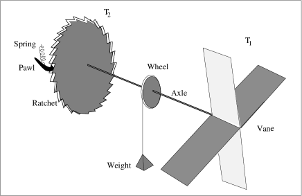
Figure 1: A schematic of Feynman’s ratchet.

The statistical fluctuations can produce a directed motion at a finite rate, only if the ratchet-pawl system is mesoscopic. Hence the pawl can undergo a Brownian motion by bouncing up and down as it is immersed in a finite temperature bath. This turns the wheel in backward direction and lowers the position of the weight. This is the reason that the system cannot work as an engine if $T_{1}=T_{2}$ [24].

The rate of the backward jumps is

$$R_{\rm B}=r_{0}e^{-\epsilon_{2}/T_{2}}.$$ (2)

Thus one can regard $Z\delta$ and $-Z\delta$ as the work done by and on the system, respectively. In an infinitesimally small time interval $\delta t$, the work done by the system is given as

$$W = (\epsilon_{1}-\epsilon_{2})(R_{\rm F}-R_{\rm B})\delta t,$$ (3)

$$= r_{0}(\epsilon_{1}-\epsilon_{2})\left(e^{-\epsilon_{1}/T_{1}}-e^{-\epsilon_{2}/T_{2}}\right)\delta t.$$

Thus the power output of the engine is defined as $P=W/\delta t$. Similarly, the rate of heat absorbed from the hot reservoir, is given as

$$\dot{Q}_{1}=r_{0}\epsilon_{1}\left(e^{-\epsilon_{1}/T_{1}}-e^{-\epsilon_{2}/T_{2}}\right),$$ (4)

or the amount of heat absorbed in the small time interval is $Q_{1}=\dot{Q}_{1}\delta t$. Then the efficiency of the engine is given by

$$\eta=\frac{W}{Q_{1}}=1-\frac{\epsilon_{2}}{\epsilon_{1}}.$$ (5)

The rate at which waste heat is rejected to the cold reservoir is $\dot{Q}_{2}=\dot{Q}_{1}-P$, which follows from the conservation of energy flux.

The power output, optimized with respect to energy scales $\epsilon_{1}$ and $\epsilon_{2}$ [25, 26], is given by

$$\tilde{P}=r_{0}e^{-1}T_{1}\eta_{c}^{2}(1-\eta_{c})^{(1-\eta_{c})/\eta_{c}}.$$ (6)

The corresponding efficiency at maximum power is

$$\tilde{\eta}=\frac{\eta_{c}^{2}}{\eta_{c}-(1-\eta_{c})\ln{(1-\eta_{c})}}.$$ (7)

Further, it was discussed in Ref. [26] that the above expression for efficiency shares some universal properties of efficiency at optimal power found in other finite-time models [1, 20].

2.1 Prior information approach

Now we consider a situation where the efficiency of the engine has some pre-specified value $\eta$, but the energy scales ($\epsilon_{1},\epsilon_{2}$) are not given to us in a priori information. Since $\eta$ is known, the problem is reduced to a single uncertain parameter, due to Eq. (5). One can cast the problem either in terms of $\epsilon_{1}$ or $\epsilon_{2}$. In terms of the latter, we can write power as

$$P(\eta,\epsilon_{2})=\frac{r_{0}\eta\epsilon_{2}}{(1-\eta)}\left(e^{-\epsilon_{2}/(1-\eta)T_{1}}-e^{-\epsilon_{2}/T_{2}}\right).$$ (8)

Analogous to quantification of prior information in Bayesian statistics, we assign a prior probability distribution for $\epsilon_{2}$ in some arbitrary, but a finite range of positive values: $[\epsilon_{\rm min},\epsilon_{\rm max}]$. Later we consider an asymptotic range in which the analysis becomes simplified and we observe universal features.

Now consider two observers $A$ and $B$ who respectively assign a prior for $\epsilon_{1}$ and $\epsilon_{2}$. Taking the simplifying assumption that each observer is in an equivalent state of knowledge, we can write [14, 18]

$$\Pi(\epsilon_{1})=\Pi(\epsilon_{2})\left|\frac{d\epsilon_{2}}{d\epsilon_{1}}\right|,$$ (9)

where $\Pi$ is the prior distribution function, taken to be of the same form for each observer. At a fixed known value of efficiency, it implies that $\Pi(\epsilon_{2})=N/\epsilon_{2}$, where the normalization constant, $N=\left[\ln\left({\epsilon_{\rm max}}/{\epsilon_{\rm min}}\right)\right]^{-1}$. This is also known as Jeffreys’ prior for a one-dimensional scale parameter [13, 14, 27].

Now the expected value of power, over this prior, is defined to be

$$\overline{P}(\eta) = \int_{\epsilon_{\rm min}}^{\epsilon_{\rm max}}P(\eta,\epsilon_{2})\Pi(\epsilon_{2})d\epsilon_{2}$$ (10)

$$= \frac{C\eta}{(1-\eta)}\int_{\epsilon_{\rm min}}^{\epsilon_{\rm max}}\left(e^{-\epsilon_{2}/(1-\eta)T_{1}}-e^{-\epsilon_{2}/T_{2}}\right)d\epsilon_{2},$$

where

$$C=r_{0}\left[\ln\left(\frac{\epsilon_{\rm max}}{\epsilon_{\rm min}}\right)\right]^{-1}.$$ (11)

Upon performing the integration, we get

$$\overline{P}(\eta) = CT_{1}\eta\left(e^{-\epsilon_{\rm min}/(1-\eta)T_{1}}-e^{-\epsilon_{\rm max}/(1-\eta)T_{1}}\right)$$ (12)

$$+\frac{CT_{2}\eta}{(1-\eta)}\left(e^{-\epsilon_{\rm max}/T_{2}}-e^{-\epsilon_{\rm min}/T_{2}}\right).$$

Now this expected power depends on the extreme values defining the range of the prior. We chose a finite range in order to define a normalized prior distribution. Otherwise, information on the finite values of these scales is not available. On the other hand, as the range is made arbitrarily large, the average power becomes increasingly small. Thus a comparison between the absolute magnitudes of optimal power (Eq. (6)) and the prior-averaged power does not seem fruitful. However, the expected power is seen to become optimal at a certain value of the given efficiency. Further, universal features are shown by this efficiency in the asymptotic limit. It also provides a good estimate of the actual values of efficiency at maximum power.

Hence, on maximizing $\overline{P}(\eta)$ with respect to $\eta$, we get

$$\frac{\partial\overline{P}}{\partial\eta} \equiv T_{1}\left(e^{-\epsilon_{\rm min}/(1-\eta)T_{1}}-e^{-\epsilon_{\rm max}/(1-\eta)T_{1}}\right)$$ (13)

$$-\frac{\eta}{(1-\eta)^{2}}\left(\epsilon_{\rm min}e^{-\epsilon_{\rm min}/(1-\eta)T_{1}}-\epsilon_{\rm max}e^{-\epsilon_{\rm max}/(1-\eta)T_{1}}\right)$$

$$+\frac{T_{2}}{(1-\eta)^{2}}\left(e^{-\epsilon_{\rm max}/T_{2}}-e^{-\epsilon_{\rm min}/T_{2}}\right)=0.$$

For given values of the limits, we obtained numerical solution for $\eta$. As shown in Fig. 2, the efficiency at maximum expected power versus $\epsilon_{\rm min}$ is plotted, for a given value of the upper limit $\epsilon_{\rm max}$. Alternately, setting the lower limit $\epsilon_{\rm min}$ as relatively small in magnitude, one can visualise the behaviour of the efficiency with $\epsilon_{\rm max}$. Interestingly, these solutions show convergence to the CA-value, $1-\sqrt{\theta}$.

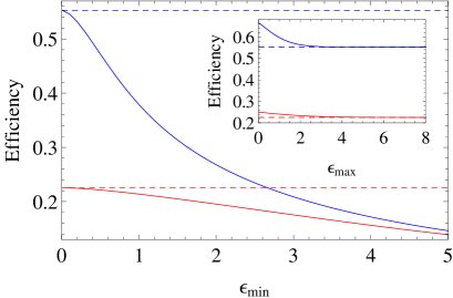
Figure 2: The efficiency at maximum expected power is plotted versus $\epsilon_{\rm min}$ (scaled by $T_{1}$), while $\epsilon_{\rm max}=10$. The upper and lower curves correspond to $\theta=0.2$ and $\theta=0.6$, respectively. The dashed lines represent corresponding CA values. The efficiency is also plotted versus $\epsilon_{\rm max}$ (inset), assuming $\epsilon_{\rm min}=0.01$. For larger values of $\epsilon_{\rm max}$, the efficiency approaches CA value.

The convergence to the CA value as observed in Fig. 1, can be argued as follows. Let us assume that the temperature gradient is not very large, i.e. $\theta$ is not close to zero. Or in other words, $\eta_{c}$ is small compared to unity. This implies that $\eta$ is also small since it is bounded from above by $\eta_{c}$. Now let us consider the limits which satisfy, $\epsilon_{\rm max}>>T_{1}$ and $\epsilon_{\rm min}<<T_{2}$ [16], referred to as asymptotic range in the following. Then the condition (13) simplifies to the form

$$T_{1}-\frac{T_{2}}{(1-\eta)^{2}}=0.$$ (14)

This implies that the efficiency at optimal $\overline{P}$, approaches the CA value.

Uniform Prior: On the other hand, maximal ignorance about the likely values of a parameter may be represented by a uniform prior density, $\Pi_{u}=1/(\epsilon_{\rm max}-\epsilon_{\rm min})$. Then the expected power, is given as

$$\overline{P}_{u}(\eta) = \int_{\epsilon_{\rm min}}^{\epsilon_{\rm max}}P(\eta,\epsilon_{2})\Pi_{u}(\epsilon_{2})d\epsilon_{2}$$ (15)

$$= \frac{C^{\prime}\eta}{(1-\eta)}\int_{\epsilon_{\rm min}}^{\epsilon_{\rm max}}\epsilon_{2}\left(e^{-\epsilon_{2}/(1-\eta)T_{1}}-e^{-\epsilon_{2}/T_{2}}\right)d\epsilon_{2},$$

where $C^{\prime}=r_{0}/(\epsilon_{\rm max}-\epsilon_{\rm min})$. Integrating the above equation, we get

$$\overline{P}_{u}(\eta) = C^{\prime}T_{1}\eta\left[(T_{1}(1-\eta)+\epsilon_{\rm min})e^{-\epsilon_{\rm min}/(1-\eta)T_{1}}\right.$$ (16)

$$\left.-(T_{1}(1-\eta)+\epsilon_{\rm max})e^{-\epsilon_{\rm max}/(1-\eta)T_{1}}\right.$$

$$\left.-\frac{T_{2}}{(1-\eta)T_{1}}\left((T_{2}+\epsilon_{\rm min})e^{-\epsilon_{\rm min}/T_{2}}-(T_{2}+\epsilon_{\rm max})e^{-\epsilon_{\rm max}/T_{2}}\right)\right].$$

Here, we are interested in the efficiency at maximum expected power ($\eta_{u}$) in the asymptotic range. Therefore, by putting $\partial\overline{P}_{u}(\eta)/\partial\eta=0$ and then considering the asymptotic limit, we get

$$(1-\eta_{u})^{2}(1-2\eta_{u})T_{1}^{2}-T_{2}^{2}=0,$$ (17)

whose real solution is given by

$$\eta_{u}=\frac{1}{6K}(5K-K^{2}-1),$$ (18)

where $K=(1+54\theta^{2}+6\sqrt{3}\theta\sqrt{1+27\theta^{2}})^{1/3}$. These efficiencies are compared in Fig. 3. In particular, we note that in the asymptotic range, the efficiency depends only on the ratio of the reservoir temperatures. Further, the use of Jeffreys’ prior gives a closer approximation to the actual behavior of efficiency at optimal performance of the engine.

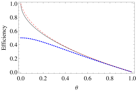
Figure 3: The solid curve shows the CA value obtained for Feynman’s ratchet at optimal expected power, using Jeffreys’ prior in the asymptotic range. The dotted curve is the corresponding efficiency (Eq. (18)) when a uniform prior is used, also in the asymptotic range. The dashed curve represents the efficiency at optimal power $\tilde{\eta}$, Eq. (7).

To compare these efficiencies near equilibrium i.e. $\eta_{c}$ close to zero, we expand these expressions as Taylor series for small values of $\eta_{c}$,

$$\tilde{\eta} = \frac{\eta_{c}}{2}+\frac{\eta_{c}^{2}}{8}+\frac{7\eta_{c}^{3}}{96}+O[\eta_{c}^{4}]\;\;({\rm Eq.(\ref{efopt})};\mbox{ at optimal power})$$ (19)

$$\eta^{*} = \frac{\eta_{c}}{2}+\frac{\eta_{c}^{2}}{8}+\frac{6\eta_{c}^{3}}{96}+O[\eta_{c}^{4}]\;\;{\rm(CA\;value\;from\;1/\epsilon_{2}\;prior)}$$ (20)

$$\eta_{u} = \frac{\eta_{c}}{2}+\frac{\eta_{c}^{2}}{16}+\frac{\eta_{c}^{3}}{64}+O[\eta_{c}^{4}].\;\;{\rm(with\;uniform\;prior)}$$ (21)

The series in Eqs. (19) and (20) were obtained in Ref. [26]. We note that $\eta_{c}/2$ term in the optimal performance can be faithfully reproduced by the expected power irrespective of the chosen prior. However, the second order term follows from the use of Jeffreys’ prior.

3 Optimal performance as a refrigerator

In this section, we consider the function of Feynman’s ratchet as a refrigerator [28, 29, 30, 31]. It is analogous to Büttiker-Landauer model [32, 33], as discussed in [29]. By optimizing the target function $\chi=\zeta\dot{Q}_{2}$ for Feynman’s ratchet, the COP at optimal performance $\tilde{\zeta}$ satisfies a transcendental equation [29]. The solution can be approximated by an interpolation formula

$$\tilde{\zeta}=\sqrt{\zeta_{c}+(0.954)^{2}}-0.954.$$ (22)

Similar to the case of heat engine, we now show using the prior based approach, that COP at optimal performance can be obtained for Feynman’s ratchet as refrigerator. The COP for certain values of $\epsilon_{1}$ and $\epsilon_{2}$ is given by $\zeta=\epsilon_{2}/(\epsilon_{1}-\epsilon_{2})$. Also the rate of refrigeration is given by

$$\dot{Q}_{2}=r_{0}\epsilon_{2}\left(e^{-\epsilon_{2}/T_{2}}-e^{-\epsilon_{1}/T_{1}}\right).$$ (23)

In terms of $\zeta$ and one of the scales say, $\epsilon_{2}$, the $\chi$-criterion is given by

$$\chi(\zeta,\epsilon_{2})=\zeta r_{0}\epsilon_{2}\left(e^{-\epsilon_{2}/T_{2}}-e^{-\epsilon_{2}(1+\zeta)/\zeta T_{1}}\right).$$ (24)

Now we suppose that the COP is fixed at some value $\zeta$, and $\epsilon_{2}$ is uncertain, within the range $[\epsilon_{\rm min},\epsilon_{\rm max}]$. Then Jeffreys’ prior for $\epsilon_{2}$ can be argued, similar to Eq. (9). Now we define the expected value of $\chi$ as

$$\overline{\chi}(\zeta) = \int_{\epsilon_{\rm min}}^{\epsilon_{\rm max}}\chi(\zeta,\epsilon_{2})\Pi(\epsilon_{2})d\epsilon_{2}$$ (25)

$$= C\int_{\epsilon_{\rm min}}^{\epsilon_{\rm max}}\zeta\left(e^{-\epsilon_{2}/T_{2}}-e^{-\epsilon_{2}(1+\zeta)/\zeta T_{1}}\right)d\epsilon_{2},$$ (26)

where $C$ is given by Eq. (11). Upon integrating the above equation, we get

$$\overline{\chi}(\zeta) = C\zeta T_{2}\left(e^{-\epsilon_{\rm min}/T_{2}}-e^{-\epsilon_{\rm max}/T_{2}}\right)$$ (27)

$$+\frac{C\zeta^{2}T_{1}}{(1+\zeta)}\left(e^{-\epsilon_{\rm max}(1+\zeta)/\zeta T_{1}}-e^{-\epsilon_{\rm min}(1+\zeta)/\zeta T_{1}}\right).$$

As with power output for the engine, the average $\overline{\chi}$ becomes increasingly small in the asymptotic limit. In the following, we focus on COP at maximal $\overline{\chi}$, in the asymptotic limit.

So the maximum of $\overline{\chi}$ with respect to $\zeta$, is evaluated as

$$\frac{\partial\overline{\chi}}{\partial\zeta} \equiv T_{2}\left(e^{-\epsilon_{\rm min}/T_{2}}-e^{-\epsilon_{\rm max}/T_{2}}\right)$$ (28)

$$+\frac{\zeta(\zeta+2)T_{1}}{(1+\zeta)^{2}}\left(e^{-\epsilon_{\rm max}(1+\zeta)/\zeta T_{1}}-e^{-\epsilon_{\rm min}(1+\zeta)/\zeta T_{1}}\right)$$

$$+\frac{1}{(1+\zeta)}\left(\epsilon_{\rm max}e^{-\epsilon_{\rm max}(1+\zeta)/\zeta T_{1}}-\epsilon_{\rm min}e^{-\epsilon_{\rm min}(1+\zeta)/\zeta T_{1}}\right)=0.$$

The numerical solution for $\zeta$ versus one of the limits is shown in Fig. 4.

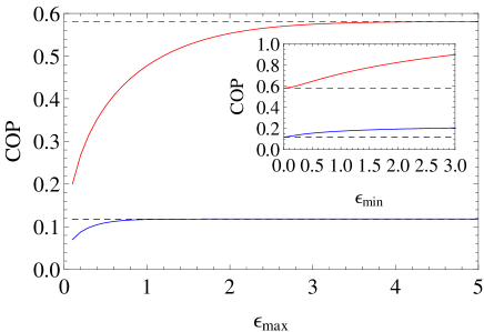
Figure 4: The COP at maximum expected $\chi$-criterion is plotted versus $\epsilon_{\rm max}$ (scaled by $T_{1}$), while $\epsilon_{\rm min}=0.01$. The upper and lower curves correspond to $\theta=0.6$ and $\theta=0.2$, respectively. The dashed lines represent corresponding $\zeta^{*}$ values. For larger values of $\epsilon_{\rm max}$, COP approaches the corresponding $\zeta^{*}$. In inset, COP is plotted versus $\epsilon_{\rm min}$, when $\epsilon_{\rm max}=10$. The COP approaches $\zeta^{*}$ as $\epsilon_{\rm min}$ takes smaller values.

Finally, in the asymptotic range, the above expression reduces to

$$\frac{\zeta(\zeta+2)}{(1+\zeta)^{2}}-\frac{T_{2}}{T_{1}}=0.$$ (29)

So the permissible solution ($\zeta>0$) of the above quadratic equation, which maximizes $\overline{\chi}$, is given as

$$\zeta^{*} = \frac{1}{\sqrt{(1-\theta)}}-1,$$ (30)

$$= \sqrt{1+\zeta_{c}}-1.$$

Uniform Prior: On the other hand, with uniform prior, the expected $\chi$-criterion is given as

$$\overline{\chi}_{u}(\zeta) = \int_{\epsilon_{\rm min}}^{\epsilon_{\rm max}}\chi(\zeta,\epsilon_{2})\Pi_{u}(\epsilon_{2})d\epsilon_{2}$$ (31)

$$= C^{\prime}\zeta\int_{\epsilon_{\rm min}}^{\epsilon_{\rm max}}\epsilon_{2}\left(e^{-\epsilon_{2}/T_{2}}-e^{-\epsilon_{2}(1+\zeta)/\zeta T_{1}}\right)d\epsilon_{2}.$$

Upon integrating the above equation, we get

$$\overline{\chi}_{u}(\zeta) = C^{\prime}\zeta\left[T_{2}\left((T_{2}+\epsilon_{\rm min})e^{-\epsilon_{\rm min}/T_{2}}-(T_{2}+\epsilon_{\rm max})e^{-\epsilon_{\rm max}/T_{2}}\right)\right.$$ (32)

$$\left.+\frac{T_{1}}{(1+\zeta)^{2}}(\epsilon_{\rm max}(1+\zeta)+\zeta T_{1})e^{-\epsilon_{\rm max}(1+\zeta)/\zeta T_{1}}\right.$$

$$\left.-\frac{T_{1}}{(1+\zeta)^{2}}(\epsilon_{\rm min}(1+\zeta)+\zeta T_{1})e^{-\epsilon_{\rm min}(1+\zeta)/\zeta T_{1}}\right].$$

Now, we want to estimate $\zeta_{u}$, the COP at maximum expected $\chi$-criterion in asymptotic range. Hence, by putting $\partial\overline{\chi}_{u}(\zeta)/\partial\zeta=0$ and imposing the asymptotic range, we obtain the following equation

$$T_{2}^{2}(1+\zeta_{u})^{3}-T_{1}^{2}\zeta_{u}^{2}(3+\zeta_{u})=0,$$ (33)

whose acceptable solution can be finally written in the following form

$$\zeta_{u}=\frac{2}{\sqrt{1-\theta^{2}}}\cos\left[\frac{\pi}{3}-\frac{\sin^{-1}\theta}{3}\right]-1.$$ (34)

Again, we see that in the asymptotic range, the COP is given only in terms of the ratio of the reservoir temperatures. We show in Fig. 5, a comparison amongst the different expressions for COP at optimized performance versus this ratio.

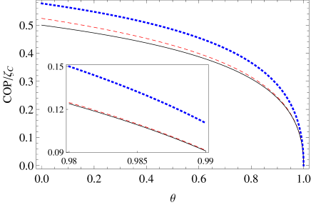
Figure 5: The COP (scaled by the Carnot value $\zeta_{c}$) is plotted versus $\theta$. The solid curve shows the COP at optimal expected performance ($\overline{\chi}$) when Jeffreys’ prior is assigned and the asymptotic range is applied. The dashed line represents the interpolation formula for COP corresponding to the optimum $\chi$ value [29]. The top, dotted line is the result of uniform prior, again in the asymptotic range. The inset shows the same three quantities for close-to-equilibrium values of $\theta$.

In near-equilibrium regime, the Carnot COP $\zeta_{c}$, as well as $\zeta^{*}$ become large in magnitude. One can then write the series expansion for $\zeta^{*}$ relative to $\zeta_{c}$ as follows:

$$\frac{\zeta^{*}}{\zeta_{c}}=\frac{1}{\sqrt{\zeta_{c}}}-\frac{1}{\zeta_{c}}+O[\zeta_{c}^{-3/2}].$$ (35)

In this case, $\zeta_{u}$ relative to $\zeta_{c}$ behaves as follows:

$$\frac{\zeta_{u}}{\zeta_{c}}=\sqrt{\frac{3}{2{\zeta_{c}}}}-\frac{4}{3\zeta_{c}}+O[\zeta_{c}^{-3/2}].$$ (36)

According to Refs. [29, 34] close to equilibrium and upto the leading order, ${\tilde{\zeta}}/{\zeta_{c}}$ behaves as $1/\sqrt{\zeta_{c}}$. The optimal behavior is thus reproduced by the use of Jeffreys’ prior, but uniform prior is not able to generate this dependence. Similarly, for large temperature differences, $\zeta_{c}\to 0$, we get the limiting behavior as $\zeta^{*}/\zeta_{c}\to 1/2$ while $\zeta_{u}/\zeta_{c}\to 1/\sqrt{3}$. The interpolation formula at optimal performance, gives $\tilde{\zeta}/\zeta_{c}\to 0.524$ [29].

Before closing this section, we point out that performing the same analysis in terms of $\epsilon_{1}$ as the uncertain scale, we obtain a similar behavior in the asymptotic range of values, and the same figures of merit, $\eta^{*}$ and $\zeta^{*}$, are obtained with the choice of Jeffreys’ prior.

4 Other Models

So far, we have focused on the performance of Feynman’s ratchet. In the following, we wish to point out that the above inference analysis can also be performed on other classes of heat engines/refrigerators [15]. The model which we discuss below is a four-step heat cycle performed by a few-level quantum system (working medium). Further, the cycle is accomplished using infinitely slow processes. The particular cycle is the quantum Otto cycle [35, 36].

Consider a quantum system with Hamiltonian $H_{1}=\sum_{n=1}^{M}\varepsilon_{n}^{(1)}|n\rangle\langle n|$, with eigenvalue spectrum of the form $\varepsilon_{n}^{(1)}=\varepsilon_{n}a_{1}$. Here $\varepsilon_{n}$ is characterised by the energy quantum number and other parameters/constants which remain fixed during the cycle. We assume there are $M$ non-degenerate levels. The parameter $a_{1}$ represents an external control, equivalent to applied magnetic field for a spin system. Initially, the system is in thermal state $\rho_{1}=\sum_{n}p_{n}^{(1)}|n\rangle\langle n|$ at temperature $T_{1}$, where $p_{n}^{(1)}=\exp(-\beta_{1}\varepsilon_{n}a_{1})/Z_{1}$, $\beta_{1}=1/k_{\rm B}T_{1}$, and the partition function $Z_{1}=\sum_{n}\exp(-\beta_{1}\varepsilon_{n}a_{1})$. The quantum Otto cycle involves the following steps [36]:

(i) The system is detached from the hot bath and made to undergo a quantum adiabatic process, in which the external control is slowly changed from the value $a_{1}$ to $a_{2}$. Thus the hamiltonian changes from $H_{1}(a_{1})$ to $H_{2}(a_{2})$ with eigenvalues $\varepsilon_{n}^{(2)}=\varepsilon_{n}a_{2}$. Following quantum adiabatic theorem, the system remains in the instantaneous eigenstate of the hamiltonian and so the occupation probabilities of the levels remain unchanged. For $a_{2}<a_{1}$, this process is the analogue of an adiabatic expansion. The work done by the system in this stage is equal to the change in mean energy ${W}_{1}={\rm Tr}(\rho_{1}[H_{2}-H_{1}])$. The change in energy spectrum is such that the ratio of energy gaps between any two levels before and after the quantum adiabatic process is the same. This makes it possible to assign temperature to the system along the adiabatic process. Thus after step (i), this temperature is given by $T_{1}(a_{2}/a_{1})$.

(ii) The system with changed spectrum $\varepsilon_{n}^{(2)}$ is brought to thermal state $\rho(a_{2})=\sum_{n}p_{n}^{(2)}|n\rangle\langle n|$ by contact with cold bath at inverse temperature $\beta_{2}$, where $p_{n}^{(2)}=\exp(-\beta_{2}\varepsilon_{n}a_{2})/Z_{2}$ and $Z_{2}=\sum_{n}\exp(-\beta_{2}\varepsilon_{n}a_{2})$. On average, the heat rejected to the bath in this step, is defined as $Q_{2}={\rm Tr}([\rho(a_{2})-\rho(a_{1})]H_{2})$.

(iii) The system is now detached from the cold bath and made to undergo a second quantum adiabatic process (compression) during which the control is reset to value $a_{1}$. Work done on the system in this step is ${W}_{2}={\rm Tr}(\rho_{2}[H_{1}-H_{2}])$.

(iv) Finally, the system is put in contact with the hot bath again. Heat is absorbed by the system in this step, whence it recovers its initial state $\rho_{1}$. On average, the total work done in one cycle, is calculated to be

$${W(a_{1},a_{2})} = \sum_{n}\left(\varepsilon_{n}^{(1)}-\varepsilon_{n}^{(2)}\right)\left(p_{n}^{(1)}-p_{n}^{(2)}\right),$$ (37)

$$= (a_{1}-a_{2})\sum_{n}\varepsilon_{n}\left(p_{n}^{(1)}-p_{n}^{(2)}\right)>0.$$ (38)

Similarly, heat exchanged with hot bath in step (iv) is given by $Q_{1}=a_{1}\sum_{n}\varepsilon_{n}\left(p_{n}^{(1)}-p_{n}^{(2)}\right)>0.$ Heat exchanged by the system with the cold bath is $Q_{2}={W}-Q_{1}<0$. The efficiency of the engine $\eta={W}/Q_{1}$, is given by

$$\eta=1-\frac{a_{2}}{a_{1}}.$$ (39)

Clearly, this cycle has two internal energy scales and the efficiency is also similar to that of Feynman’s ratchet, Eq. (5). One can seek an optimal engine configuration, by optimising work output per cycle over the parameters $a_{1}$ and $a_{2}$. However, unlike the case of Feynman’s ratchet as engine, a closed-form expression for the efficiency at optimal work seems difficult to obtain here [37].

We can formulate a problem of estimation here, for performance of the engine, assuming that the absolute magnitudes of internal scales are not known. Further, we simplify by assuming that the ratio of energy scales, or in other words, the efficiency is specified. In the following, we briefly outline the emergence of CA efficiency in this problem. The following treatment generalizes the analysis of Ref. [15].

It is convenient to express ${W(a_{1},a_{2})}\equiv{W}(a_{1},\eta)$, using Eq. (39). Due to analogy with the ratchet problem, we may take the prior for the uncertain parameter $a_{1}$ to be Jeffreys’ prior: $\Pi(a_{1})=N/a_{1}$, where $N=[\ln(a_{\rm max}/a_{\rm min})]^{-1}$. The expected work per cycle for a given $\eta$, is then given by

$$\overline{W}(\eta) = \int_{a_{\rm min}}^{a_{\rm max}}{W}(a_{1},\eta)\Pi(a_{1})da_{1}$$ (40)

$$= N\eta\int_{a_{\rm min}}^{a_{\rm max}}\sum_{n}\varepsilon_{n}\left(p_{n}^{(1)}-p_{n}^{(2)}\right)da_{1}$$ (41)

To perform the integration, we write $\int\sum_{n}\varepsilon_{n}p_{n}^{(1)}da_{1}=\sum_{n}\varepsilon_{n}\int p_{n}^{(1)}da_{1}$ and integrate by parts. The result can be written as:

$$\sum_{n}\varepsilon_{n}\int_{a_{\rm min}}^{a_{\rm max}}p_{n}^{(1)}da_{1}=-\frac{1}{\beta_{1}}\ln\left(\frac{\sum_{k=1}^{M}e^{-\beta_{1}\varepsilon_{k}a_{\rm max}}}{\sum_{k=1}^{M}e^{-\beta_{1}\varepsilon_{k}a_{\rm min}}}\right).$$ (42)

Thus the average work is evaluated to be

$$\overline{W}=N\eta\left[\frac{1}{\beta_{2}(1-\eta)}\ln\left(\frac{\sum_{k}e^{-\beta_{2}(1-\eta)\varepsilon_{k}a_{\rm max}}}{\sum_{k}e^{-\beta_{2}(1-\eta)\varepsilon_{k}a_{\rm min}}}\right)-\frac{1}{\beta_{1}}\ln\left(\frac{\sum_{k}e^{-\beta_{1}\varepsilon_{k}a_{\rm max}}}{\sum_{k}e^{-\beta_{1}\varepsilon_{k}a_{\rm min}}}\right)\right],$$ (43)

or, which is written briefly as:

$$\overline{W}=N\eta\left[\frac{X_{2}}{\beta_{2}(1-\eta)}-\frac{X_{1}}{\beta_{1}}\right],$$ (44)

where $X_{1}$ and $X_{2}$ can be easily identified from Eq. (43).

Now we wish to find the efficiency at optimal average work, and so we apply the condition

$$\frac{\partial\overline{W}}{\partial\eta}=0\quad\Longrightarrow\quad\frac{X_{2}}{\beta_{2}(1-\eta)^{2}}-\frac{X_{1}}{\beta_{1}}+\frac{\eta}{\beta_{2}(1-\eta)}\frac{\partial X_{2}}{\partial\eta}=0.$$ (45)

The resulting equation is, in general, a function of $a_{\rm max}$ and $a_{\rm min}$. However, we are interested in the asymptotic limit of large $a_{\rm max}$ and vanishing $a_{\rm min}$. In this limit, the dominant term in the sum $\sum_{k}e^{-\beta_{2}(1-\eta)\varepsilon_{k}a_{\rm max}}$ is given by $e^{-\beta_{2}(1-\eta)\varepsilon_{1}a_{\rm max}}$, where $\varepsilon_{1}$ is the ground-state energy. Therefore, $X_{2}\to-\beta_{2}(1-\eta)\varepsilon_{1}a_{\rm max}-\ln M$. Similarly, in the said limit

$$X_{1}\to-\beta_{1}\varepsilon_{1}a_{\rm max}-\ln M,\quad\frac{\partial X_{2}}{\partial\eta}\to\beta_{2}\varepsilon_{1}a_{\rm max}.$$ (46)

Finally, using the above limiting forms in Eq. (45), we obtain:

$$\ln M\left[\frac{1}{\beta_{1}}-\frac{1}{\beta_{2}(1-\eta)^{2}}\right]=0,$$ (47)

which implies that the expected work becomes optimal at $\eta=1-\sqrt{\frac{\beta_{1}}{\beta_{2}}}$, or at CA-efficiency.

5 Summary

We observed in Feynman’s ratchet that for small temperature differences, the figures of merit at optimal values of $\overline{P}$ and $\overline{\chi}$, agree with the corresponding expressions at the optimal values of $P$ and $\chi$. The important conditions which hold in this comparison are, Jeffreys’ prior as the underlying prior and an asymptotic range of values over which the prior is defined. In contrast, the uniform prior is not able to generate the optimal behavior in the near equilibrium regime. Further we note that for endoreversible models with a Newtonian heat flow between a reservoir and the working medium, the efficiency at optimal power is exactly $\eta^{*}$ [1, 38]. Correspondingly, the COP at optimal $\chi$-criterion is given by $\zeta^{*}$ [7]. In this paper, these values are obtained with an inference based approach assuming incomplete information in a mesoscopic model of heat engine. We have also shown that our analysis applies to a broader class of idealized models of heat engines/refrigerators, driven by quasi-static processes. Here also, CA efficiency emerges from the use of Jeffreys’ prior, under the given conditions of the model.

We conclude with an argument to support as to why our approach yields the familiar results of finite-time thermodynamics. To exemplify, in the case of Feynman’s ratchet, the asymptotic range has been considered after we optimized the expected power output (in case of engine) over the efficiency. One may consider these two steps in the opposite order, i.e. take the asymptotic range first and then perform the optimization. For that we rewrite Eq. (4) as follows:

$$\dot{Q}_{1}(\epsilon_{2},\eta)=\frac{r_{0}\epsilon_{2}}{(1-\eta)}\left(e^{-\epsilon_{2}/(1-\eta)T_{1}}-e^{-\epsilon_{2}/T_{2}}\right),$$ (48)

and define the expected heat flux as

$$\overline{\dot{Q}}_{1}=\int_{\epsilon_{\rm min}}^{\epsilon_{\rm max}}\dot{Q}_{1}(\epsilon_{2},\eta)\Pi(\epsilon_{2})d\epsilon_{2}.$$ (49)

Then in the asymptotic range, we obtain the approximate expression as

$$\overline{\dot{Q}}_{1}\approx C\left[T_{1}-\frac{T_{2}}{1-\eta}\right],$$ (50)

where $C$ is as in Eq. (11). Here we can draw a parallel with Newtonian heat flow: $\overline{\dot{Q}}_{1}\propto[T_{1}-T_{1}^{\prime}]$ where $T_{1}^{\prime}\equiv{T_{2}}/{(1-\eta)}<T_{1}$ is an effective temperature. Similarly, the prior-averaged rate of heat rejected to the cold reservoir can be written as

$$\overline{\dot{Q}}_{2}\approx C\left[(1-\eta){T_{1}}-T_{2}\right].$$ (51)

Here also, we may identify another Newtonian heat flow $\overline{\dot{Q}}_{2}\propto[T_{2}^{\prime}-T_{2}]$, with the same effective heat conductance $C$, between an effective temperature $T_{2}^{\prime}\equiv(1-\eta){T_{1}}>T_{2}$ and temperature $T_{2}$ of the cold reservoir. Then it is easily seen that the maximum of expected power $\overline{P}=\overline{\dot{Q}}_{1}-\overline{\dot{Q}}_{2}$, is obtained at CA value. Similarly, one can argue for the emergence of $\zeta^{*}$ in the case of refrigerator mode, in terms of effective heat flows which are Newtonian in nature.

Interestingly, the above expressions seem to suggest an analogy between the expected mesoscopic model with limited information, and a finite-time thermodynamic model with Newtonian heat flows. If we compare with the endoreversible models [1, 7], then we observe that the assumption of a Newtonian heat flow goes together with obtaining CA efficiency at maximum power, and COP $\zeta^{*}$ at optimum $\chi$-criterion. We however note that the analogy does not hold in entirety. The effective temperatures defined above do not have physical counterpart in the ratchet model, although in the endoreversible picture, these denote the temperatures of the working medium while in contact with hot or cold reservoirs. Secondly, the heat conductances need not be equal for the endoreversible model with Newtonian heat flows. Further, the intermediate temperatures $T_{1}^{\prime}$ and $T_{2}^{\prime}$ as above, are equal in magnitude at the maximum expected power $\overline{P}$. However, for the endoreversible model, these temperatures are not equal at maximum power [1, 38]. Still, the form of expressions for the rates of heat transfer do provide a certain insight into the emergence of the familiar expressions for figures of merit at optimal expected performance within the prior-averaged approach.

Finally, we close with a few observations on future lines of enquiry. It was seen in Fig. 1, that for a specified finite range for the prior, the estimates of efficiency at maximum power are either above, or below the estimates in the asymptotic range. In particular, the estimates are function of the values $\epsilon_{\rm min}$ and $\epsilon_{\rm max}$. We obtain universal results, dependent on the ratio of reservoir temperatures, only in the asymptotic range. Further, the smaller values of the upper limit, overestimate the efficiency (inset in Fig. 1) whereas the larger values of the lower limit, underestimate the efficiency. An opposite behavior is seen for the refrigerator mode (Fig. 4). Moreover, this trend for a chosen mode (engine/refrigerator) is specific to the choice of the uncertain variable. Thus the trend is reversed, if instead of choosing $\epsilon_{2}$, we perform the analysis with $\epsilon_{1}$ as the uncertain variable. This behavior is seen in both the engine as well as the refrigerator mode. Investigation into the relation between inferences derived from the two choices for the uncertain variable, may yield further insight into the behavior of estimated performance and the approach in general. The point may be appreciated by noting that by specifying a finite-range for the prior we add new information to the probabilistic model. In order that inference may provide a useful and practical guess on the actual performance of the device, this additional prior information has to be related to some objective features of the model. These considerations are relevant for further exploring the intriguing relation between the subjective and the objective descriptions of thermodynamic models [23].

6 Acknowledgement

The authors acknowledge financial support from the Department of Science and Technology, India under the research project No. SR/S2/CMP-0047/2010(G), titled: “Quantum Heat Engines: work, entropy and information at the nanoscale”.

References

- [1] F. L. Curzon, B. Ahlborn, Efficiency of a Carnot engine at maximum power output, Am. J. Phys. 43 (1975) 22.
- [2] A. De Vos, Endoreversible Thermodynamics of Solar Energy Conversion, Oxford science publications, Oxford University Press, Oxford, 1992.
- [3] P. Salamon, J. Nulton, G. Siragusa, T. Andersen, A. Limon, Principles of control thermodynamics, Energy 26 (3) (2001) 307.
- [4] M. Esposito, R. Kawai, K. Lindenberg, C. Van den Broeck, Efficiency at maximum power of low-dissipation Carnot engines, Phys. Rev. Lett. 105 (2010) 150603.
- [5] C. Van den Broeck, Thermodynamic efficiency at maximum power, Phys. Rev. Lett. 95 (2005) 190602.
- [6] M. Esposito, K. Lindenberg, C. Van den Broeck, Universality of efficiency at maximum power, Phys. Rev. Lett. 102 (2009) 130602.
- [7] Z. Yan, J. Chen, A class of irreversible Carnot refrigeration cycles with a general heat transfer law, J. Phys. D: Appl. Phys. 23 (2) (1990) 136.
- [8] Y. Apertet, H. Ouerdane, A. Michot, C. Goupil, P. Lecoeur, On the efficiency at maximum cooling power, Europhys. Lett. 103 (4) (2013) 40001.
- [9] A. E. Allahverdyan, K. Hovhannisyan, G. Mahler, Optimal refrigerator, Phys. Rev. E 81 (2010) 051129.
- [10] C. de Tomás, A. C. Hernández, J. M. M. Roco, Optimal low symmetric dissipation Carnot engines and refrigerators, Phys. Rev. E 85 (2012) 010104.
- [11] Y. Wang, M. Li, Z. C. Tu, A. C. Hernández, J. M. M. Roco, Coefficient of performance at maximum figure of merit and its bounds for low-dissipation carnot-like refrigerators, Phys. Rev. E 86 (2012) 011127.
- [12] Y. Hu, F. Wu, Y. Ma, J. He, J. Wang, A. C. Hernández, J. M. M. Roco, Coefficient of performance for a low-dissipation Carnot-like refrigerator with nonadiabatic dissipation, Phys. Rev. E 88 (2013) 062115.
- [13] H. Jeffreys, Theory of Probability, Clarendon Press, Oxford, 1939.
- [14] E. Jaynes, Prior probabilities, IEEE Trans. Syst. Sci. Cybernet. 4 (1968) 227.
- [15] R. S. Johal, Universal efficiency at optimal work with Bayesian statistics, Phys. Rev. E 82 (2010) 061113.
- [16] G. Thomas, R. S. Johal, Expected behavior of quantum thermodynamic machines with prior information, Phys. Rev. E 85 (2012) 041146.
- [17] G. Thomas, P. Aneja, R. S. Johal, Informative priors and the analogy between quantum and classical heat engines, Physica Scripta (T151) (2012) 014031.
- [18] P. Aneja, R. S. Johal, Prior information and inference of optimality in thermodynamic processes, J. Phys. A: Math. Theor. 46 (36) (2013) 365002.
- [19] R. S. Johal, Efficiency at optimal work from finite source and sink: a probabilistic perspective, J. Noneq. Therm. 40 (2015) 1.
- [20] T. Schmiedl, U. Seifert, Efficiency at maximum power: An analytically solvable model for stochastic heat engines, Europhys. Lett. 81 (2) (2008) 20003.
- [21] Y. Zhang, B. H. Lin, J. C. Chen, Performance characteristics of an irreversible thermally driven Brownian microscopic heat engine. Eur. Phys. J. B 53 (2006) 481.
- [22] A. C. Barato, U. Seifert, An autonomous and reversible Maxwell’s demon. Europhys. Lett. 101 (2013) 60001.
- [23] R. S. Johal, R. Rai, G. Mahler, Reversible heat engines: Bounds on estimated efficiency from inference, Found. Phys. 45 (2015) 158.
- [24] R. P. Feynman, R. B. Leighton, M. Sands, The Feynman Lectures on Physics, Addison-Wesley, Reading, MA, 1966.
- [25] S. Velasco, J. M. M. Roco, A. Medina, A. C. Hernández, Feynman’s ratchet optimization: maximum power and maximum efficiency regimes, J. Phys. D: Appl. Phys. 34 (6) (2001) 1000.
- [26] Z. C. Tu, Efficiency at maximum power of Feynman’s ratchet as a heat engine, J. Phys. A: Math. Theor. 41 (31) (2008) 312003.
- [27] S. Abe, Conditional maximum-entropy method for selecting prior distributions in Bayesian statistics, Europhys. Lett. 108 (2014) 40008.
- [28] X. G. Luo, N. Liu, J. Z. He, Optimum analysis of a Brownian refrigerator, Phys. Rev. E 87 (2013) 022139.
- [29] S. Sheng, P. Yang, Z. C. Tu, Coefficient of performance at maximum -criterion for Feynman ratchet as a refrigerator, Commun. Theor. Phys. 62 (2014) 589.
- [30] B.-Q. Ai, L. Wang, L.-G. Liu, Brownian micro-engines and refrigerators in a spatially periodic temperature field: Heat flow and performances, Phys. Lett. A 352 (4–5) (2006) 286.
- [31] B. Lin, J. Chen, Performance characteristics and parametric optimum criteria of a brownian micro-refrigerator in a spatially periodic temperature field, J. Phys. A: Math. Theor. 42 (7) (2009) 075006.
- [32] M. Büttiker, Transport as a consequence of state-dependent diffusion, Zeitschrift für Physik B Condensed Matter 68 (2-3) (1987) 161.
- [33] R. Landauer, Motion out of noisy states, J. Stat. Phys. 53 (1-2) (1988) 233.
- [34] S. Sheng, Z. C. Tu, Universality of energy conversion efficiency for optimal tight-coupling heat engines and refrigerators, J. Phys. A: Math. Theor. 46 (40) (2013) 402001.
- [35] T.D. Kieu, Quantum heat engines, the second law and Maxwell’s daemon, Eur. Phys. J. D 39 (2006) 115.
- [36] H.T. Quan,Yu-xi Liu, C. P. Sun, and Franco Nori, Quantum thermodynamic cycles and quantum heat engines, Phys. Rev. E 76 (2007) 031105.
- [37] A. Allahverdyan, R.S. Johal, G. Mahler, Work extremum principle: Structure and function of quantum heat engines, Phys. Rev. E 77 (2008) 041118.
- [38] G. Lebon, D. Jou, J. Casas-Vásquez, Understanding Nonequilibrium Thermodynamics, Springer, Berlin, 2008.